Intelligence modeling of the flow boiling heat transfer of nanorefrigerant for integrated energy system

Highlights

(1) Four intelligence models—RBF, MLP, LSSVM, and ANFIS—for predicting the flow boiling HTC of nanorefrigerants with satisfactory performance, are developed based on 765 experimental data samples.

(2) The RBF model outperformed all of the other intelligence and empirical models.

(3) The RBF model accurately captured the variation trends of the output as the input parameters.

(4) The impact degrees of each independent input on the output of the model is evaluated.

1 Introduction

As an effective method to reduce the energy consumption and carbon emissions, the Integrated Energy System (IES) has been paid attention by more and more countries during the past several decades. As the advanced technical and management approaches are being adopted, the different types of energy, such as coal, oil, natural gas, electricity and heat, can be utilized effectively and economically in IES (Ngangu’e et al., 2023). In China, the development of IES technology is of great significance to achieve carbon neutrality (Kang et al., 2023). For IES and CCHP (Combined Cooling, Heating, and Power) systems, the commonly used subsystems are the Organic Rankine Cycle (ORC) and the Vapor Compression Refrigeration Cycle (VCR). The ORC systems are composed of an evaporator, turbine, condenser, and working fluid pump, and typically utilize the organic fluid with low boiling points, such as refrigerants and hydrocarbons, as the working fluid. This allows for the effective extraction of heat from moderate to low-grade heat sources, to produce the electricity effectively (Feng et al., 2024). Similarly, VCR systems consist of an evaporator, compressor, condenser, and expansion valve, facilitating the continuous cyclic motion and phase transitions of the refrigerant, which enables heat exchange with the external environment. Nonetheless, the heat transfer efficiency in ORC and VCR systems is significantly hindered by the relatively low thermal conductivity of the organic media (or refrigerants), which stands at merely one-tenth that of water, particularly impacting the performance of evaporators. This poses a considerable challenge to enhancing the technical and economic feasibility of IES systems. Given that both ORC and VCR systems can operate using various refrigerants (e.g., R123, R245fa, R141b, R600a) as the working fluid and share similarities in system composition, it is projected that utilizing advanced technical methods to enhance the heat transfer coefficients of the working fluid could lead to simultaneous enhancements in the energy efficiency and techno-economic performance of both ORC and VCR systems (Kumar et al., 2022).

Flow boiling heat transfer is widely applied in the fields of power generation, VCR, ORC, thermal management, steam generation, ultra cooling, chemical engineering, and nuclear reactors. With the continuous advancement in nanotechnology and the rising demand for heat transfer enhancement, nanofluid was proposed by Choi and Eastman from the U. S. Argonne National Laboratory in 1995 (Choi and Eastman, 1995). Similar to that of nanofluid, nanorefrigerant is a mixture of solid nanoparticles and liquid refrigerants, such as HFC-245fa, HCFC-141b, HCFC-123, et al. (Yilmaz et al., 2024). Relevant investigation on the thermophysical properties (Said et al., 2023), flow boiling heat transfer (Peng et al., 2009; Sun and Yang, 2013; Akhavan-Behabadi et al., 2014; Baqeri et al., 2014; Sun and Yang, 2014; Yang et al., 2015; Zhang et al., 2016; Sheikholeslami et al., 2019), flow condensation (Kumar et al., 2024) and practical applications (Kosmadakis and Neofytou, 2020; Dey and Mandal, 2021) of nanorefrigerants has demonstrated their potential to enhance the heat transfer while reducing the power consumption of fluid pump.

Grasping the knowledge of the flow boiling heat transfer coefficient (HTC) of nanorefrigerants is essential for promoting the application of nanorefrigerants in IES. To date, relevant research results have indicated that the flow boiling HTC of nanorefrigerants are significantly higher than those of pure refrigerants. Meanwhile, the flow boiling HTC is mainly influenced by the nanoparticle volume concentration (φ_v), mass flux (G), vapor quality (x), thermal conductivity of nanoparticles (k_p), and et al. (Peng et al., 2009; Sun and Yang, 2013; Akhavan-Behabadi et al., 2014; Baqeri et al., 2014; Sun and Yang, 2014; Zhang et al., 2016). The experimental measurements have proved to be a reliable research method in the field of nanofluid, however, the experimental process is costly and extremely time-consuming (Hemmati-Sarapardeha et al., 2018; Huang et al., 2024). For this reason, it is necessary to establish a mathematical correlation for predicting the flow boiling HTC of nanorefrigerants with high accuracy.

In the existing relevant research literature, two correlations were proposed by researchers to predicate the flow boiling HTC of nanorefrigerants (Peng et al., 2009; Zhang et al., 2016). Based on the experimental results of flow boiling using CuO-R113 nanorefrigerant, Peng proposed an empirical correlation for predicting the flow boiling HTC of nanorefrigerants within the deviation of ±20% (Peng et al., 2009). Peng’s correlation can be expressed as:

$h_{\text{fb},\text{nf}}=F_{\text{ht}}\cdot h_{\text{fb},\text{bf}}(1)$

$F_{\text{ht}}=\exp \left\{{\phi }_{\mathrm{v}}\left[0.8\frac{k_{\mathrm{p}}}{k_{\text{bf}}}-39.94\frac{\left({\rho }_{\mathrm{p}}\cdot C_p{,}_{\mathrm{p}}\right)}{\left({\rho }_{\text{bf}}\cdot C_p{,}_{\text{bf}}\right)}-0.028G-733.26x\left(1-x\right)\right]\right\}(2)$

where, h_{fb, nf} and h_{fb, bf} denote the flow boiling HTC of nanorefrigerant and pure refrigerant, respectively (W/m²·K); F_ht denotes the nanoparticle impact factor, defined as the ratio of HTC between the nanorefrigerants and pure refrigerant (F_ht = h_fb,nf/h_fb,bf); k, ρ, φ, and C_p denote the thermal conductivity (W/m·K), density (kg/m³), nanoparticle concentration, and specific heat (J/kg·K), respectively; the subscripts p, bf, and nf denote the nanoparticle, pure refrigerant, and nanorefrigerant, respectively; G denote the mass flux (kg/m²·s); and x denote the vapor quality.

Zhang et al. (Zhang et al., 2016) proposed a modified correlation to predict the flow boiling F_ht of nanorefrigerants, based on the experimental data of multiwalled carbon nanotubes (MWCNTs)–R123 nanorefrigerants. Zhang’s correlation can be expressed as:

$F_{\text{ht}}=\exp \left\{{\phi }_{\mathrm{v}}\left[894.3{\left(\frac{k_{\text{nf}}}{k_{\text{bf}}}\right)}^{0.6}{\left(\frac{{\mu }_{\text{nf}}}{{\mu }_{\text{bf}}}\right)}^{-0.4}{\left(\frac{\left({\rho }_{\text{nf}}\cdot C_p{,}_{\text{nf}}\right)}{\left({\rho }_{\text{bf}}\cdot C_p{,}_{\text{bf}}\right)}\right)}^{0.4}+1171x\left(1-x\right)-0.011Re-908.3\right]]\right\}\}(3)$

where, μ denote the dynamic viscosity (Pa·s); and Re denote the Reynolds number.

However, the application scope of the above two correlations is very limited, due to the complexity of the nanoparticle–liquid suspensions. Meanwhile, both of the correlations were proposed based on limited experimental conditions and experimental data. Whether these correlations can be applied to other conditions and different nanofluid type with acceptable accuracy, is still a question.

In the last few decades, intelligence models have been proved to be an effective method in dealing with the complex non-linear problems due to the advantages of high accuracy, favorable speed, broad applicability, feature extraction, adaptive, fault tolerance, and simple structure (Hemmati-Sarapardeh et al., 2020; Zarei et al., 2020). The flow boiling heat transfer of nanofluids is suitable for computation with intelligence model. The frequently used intelligence models are Radial Basis Function (RBF), Multi-Layer Perceptron (MLP), Least‒Squares Support‒Vector Machine (LSSVM), and Adaptive Neuro Fuzzy Inference System (ANFIS). In the study of Zarei et al. (Zarei et al., 2020), an MLP model with various training algorithms were developed to predict the pool boiling HTC of nanorefrigerants. A total of 1,342 experimental data were used. Results indicated that the root mean square error (RMSE) between the predicted value and the experimental one was 0.01529. The optimum structure was one hidden layer which contained 19 neurons, trained by the Levenberg-Marquardt (LM) algorithm. In the study of Hemmati‒Sarapardeh et al. (Hemmati-Sarapardeh et al., 2020), the MLP, RBF, and LSSVM models were developed to predict the thermal conductivities of nanofluids. A total of 3,200 experimental data were utilized. Dadhich et al. (Dadhich et al., 2020) developed an MLP model to predict the nanoparticle impact factor (F_ht) of water-based nanofluids containing TiO₂ and Al₂O₃ nanoparticle flow boiling inside an annulus copper tube. The results showed that the accuracy of the MLP model were superior to the empirical correlations. Kanti et al. (Kanti et al., 2022) utilized the RBF based neural network to predict s dynamic viscosity and thermal conductivity of fly ash-copper (80:20% by vol.) hybrid nanofluid. The results indicated that the RBF model optimizes the viscosity and thermal conductivity of the hybrid nanofluid with R² values 0.9963 and 0.9962, respectively. In the study of Ghadery-Fahliyany et al. (Fahliyany et al., 2024), three optimized intelligent models on the basis of multilayer perceptron (MLP), two radial basis function (RBF) models (including RBF- particle swarm optimization (PSO) and RBF- farmland fertility algorithm (FFA)), and a committee machine intelligent system (CMIS) were used to estimate thermal conductivity of hybrid nanofluids. A total number of 504 experimental data points for 26 hybrid nanofluids were collected from the existing literature. The results indicated that the CMIS model emerged as the most accurate model for predicting thermal conductivity of hybrid nanofluids.

According to the literature review, most of previous studies were focused on the thermophysical properties and heat transfer using the non-refrigerants (water, EG, acetone, and et al.) based nanofluids. Predicting the flow boiling HTC of nanorefrigerants by means of artificial intelligence approach, has not been reported at present. Owing to the intrinsic complexity of flow boiling heat transfer using nanorefrigerants, experimental data which covered a wide range of experimental conditions are necessary to develop a reliable model. Further, to promote the application of nanorefrigerant in ORC, refrigeration, and IES, a reliable model with simple structure and favorable accuracy for predicting the flow boiling HTC of nanorefrigerant is essential.

In this work, for the first time, artificial intelligence models including RBF, MLP, LSSVM, and ANFIS were proposed to predict the flow boiling HTC of nanorefrigerants. A total number of 765 experimental samples relevant to flow boiling heat transfer using nanorefrigerant were collected from the published literature. To comprehensively assess the reliability of the models, the accuracies of the proposed intelligence models and the existing empirical correlations were analyzed from several aspects. Meanwhile, variation trend and sensitivity were analyzed to assess the impact of each input parameter on the output. It is believed that the results of this work will lay a certain foundation for practical applications of nanorefrigerants in the ORC, refrigeration, and IES. The research approach of this work is shown in Figure 1

Figure 1

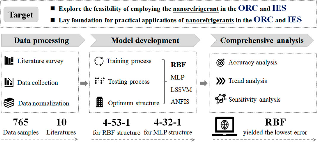
Figure 1. The research approach of this work.

The novelties of this work were highlighted as follows:

(1) A new thought for improving the heat transfer performance and the total energy efficiency of ORC and IES by utilizing the nanorefrigerants, was proposed.

(2) Novel prediction methods for predicting the heat transfer coefficient of nano-refrigerants under flow boiling condition based on the intelligence models (RBF, MLP, LSSVM, and ANFIS), were developed, optimized and compared, for the first time.

(3) Dataset with a total number of 765 experimental data samples which covering a wide range of nanoparticle material, nanoparticle concentration, mass flux, and vapor quality from various existing literature were collected.

(4) The comprehensive performances including accuracies, robustness, physical variation, and sensitivity of the four intelligence models were assessed and compared in detail, and the model with the best performance was selected.

2 Data processing

2.1 Data collection

In this work, a total of 765 experimental data samples were gathered from 10 available research literature [2, 7, 11‒14, 17, 24‒26]. The type of refrigerants collected in this work included R113, R123, R134a, R141b, and R600a. The type of nanoparticles collected in this work included Al, Al₂O₃, Cu, CuO, SiO₂, TiO₂, and MWCNTs. The concentration of the nanoparticle (φ), mass flux of the nanorefrigerant (G), vapor quality (x), and thermal conductivity of the nanoparticle (k_p) were considered as the input parameters. The nanoparticle impact factor F_ht (F_ht = h_fb,nf/h_fb,bf) was considered as the output targe. Relevant parameters in the reference literature are tabulated in Table 1. The statistic description of the data samples used for developing the intelligence models are tabulated in Table 2.

Table 1

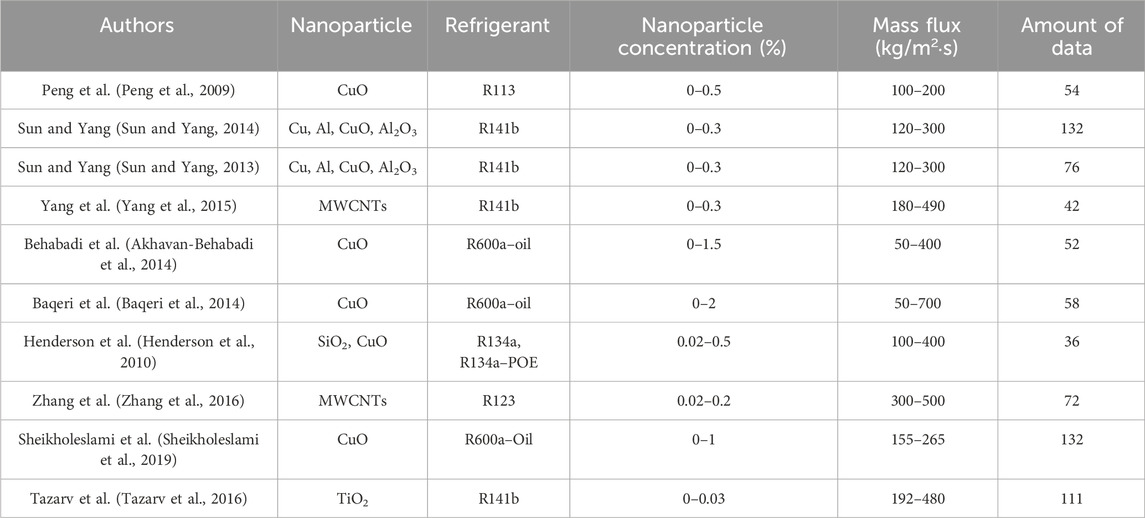
Table 1. Relevant parameters of flow boiling HTC using nanorefrigerants in the literature.

Table 2

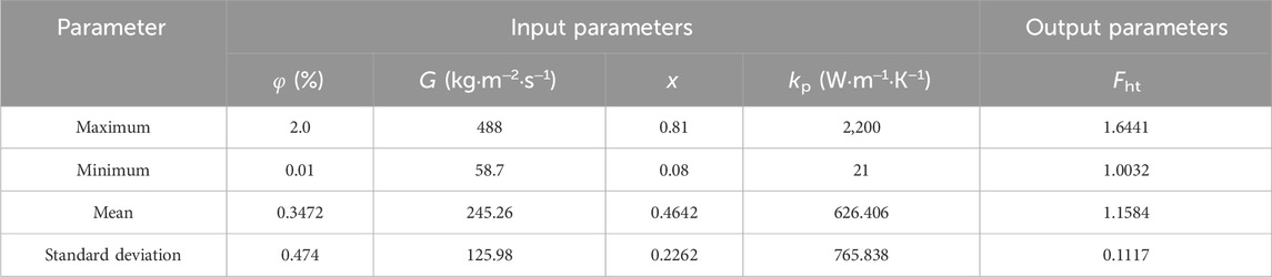
Table 2. Statistic analysis of the collected experimental samples.

In the modeling process, the initial data samples should be normalized by employing the following formula:

$x^{\prime }=\frac{x-x_{\min }}{x_{\max }-x_{\min }}(4)$

where, x′ and x denote the normalized data and the initial data, respectively; the subscript of max and min denote the maximum values and the minimum values, respectively.

Meanwhile, to prevent excessive aggregation of data in local area, 574 data samples (75%) were randomized to the training set, and 191 data samples (25%) were randomized to the testing set.

2.2 Performance evaluation parameter

To comprehensively assess the developed intelligence models quantitatively, the following performance evaluation parameters were utilized and were given as follows:

Determination Coefficient (R²)

$R^2=1-\frac{{\displaystyle \sum _{i=1}^N}{\left(F_{\text{ht},\exp ,i}-F_{\text{ht},\text{pre},i}\right)}^2}{{\displaystyle \sum _{i=1}^N}{\left(F_{\text{ht},\exp ,i}-{\overline{F}}_{\text{ht},\exp }\right)}^2}(5)$

Root-Mean-Squared-Error (RMSE)

$\text{RMSE}=\sqrt{\frac{1}{N}{\displaystyle \sum _{i=1}^N}{\left(F_{\text{ht},\exp ,i}-F_{\text{ht},\text{pre},i}\right)}^2}(6)$

Mean-Squared-Error (MSE)

$\text{MSE}=\frac{1}{N}{\displaystyle \sum _{i=1}^N}{\left(F_{\text{ht},\exp ,i}-F_{\text{ht},\text{pre},i}\right)}^2(7)$

Mean-Absolute-Percentage-Error (MAPE, %)

$\text{MAPE}\%=\frac{100}{N}{\displaystyle \sum _{i=1}^N}\left|\frac{F_{\text{ht},\exp ,i}-F_{\text{ht},\text{pre},i}}{F_{\text{ht},\exp ,i}}\right|(8)$

where, F_{ht, exp} and F_{ht, pre} denote the experimental value and the predicted value of nanoparticle impact factor, respectively. F_{ht, exp} denote the average value of the nanoparticle impact factor, and N denote the total number of the data samples. In simple terms, the best fit between the experimental and predicted values would have R² = 1, RMSE = 0, MSE = 0, and MAPE% = 0.

3 Modeling process

3.1 Radial basis function (RBF)

As a typical artificial neural network based on the function approximation method, RBF model high convergence rate, good precision, and simply form. The basic structure of RBF is consisted of three fixed layers: an input layer, a hidden layer, and an output layer (Yu et al., 2008). Each layer contains a different number of neurons and is connected by weights and bias. The number of neurons in the input layer (l) is equal to the number of input variables in the model (l = 4). The input layer first receives the input vectors and then transmits them to the hidden layer. Then, the data from the input layer are activated, processed and transmitted to the output layer, by means of an activation function in the hidden layer. Finally, the output of the kth neurons in the output layer y_k, can be expressed as:

$y_k={\displaystyle \sum _{j=1}^m}{w}_{jk}{\varphi }_j\left(r\right),\left(k=1,2,\dots ,n\right)(9)$

where w_jk denotes the weight connecting the jth neuron in the hidden layer and the kth neuron in the output layer, which can be determined in the training process; m denotes the number of neurons in the hidden layer, and n denotes the number of neurons in the output layer, which is equal to the number of outputs in the model (n = 1); ϕ denotes the activation function in the RBF model, which is selected as a Gaussian function and is expressed as:

${\varphi }_j\left(r_{\mathrm{E}}\right)=\varphi \left(r_{\mathrm{E},j}\right)=e^{\left(-\frac{{r_{\mathrm{E},j}}^2}{2{{\sigma }_j}^2}\right)}(10)$

where σ denote the Spread coefficient, and r_E denotes the Euclidian distance. The Euclidian distance between the ith neuron in the input layer (x_i) and the jth neuron in the hidden layer (c_ij), can be calculated as:

$r_{\mathrm{E},j}=‖x_i-c_{ij}‖=\sqrt{{\displaystyle \sum _{i=1}^l}{\left(x_i-c_{ij}\right)}^2}\left(i=1,\dots ,l,j=1,2,\dots ,m\right)(11)$

So far, the basic structure of the developed RBF model can be obtained as 4−m−1. To achieve the optimum performance of the RBF model, it is critical to determine the values of m, σ, weights, and bias. By comprehensive comparison, trial and error is utilized to determine the optimum values of m and σ. Meanwhile, to determine the optimum combinations of weights and biases, the Orthogonal Least Squares (OLS) and an Adaptive Gradient Descent Algorithm are utilized for training the RBF model. Variations of the performance parameters in the training and testing process are tabulated in Table 3.

Table 3

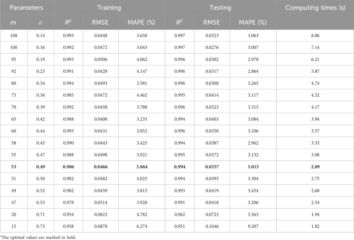
Table 3. Variations of the performance parameters in the training and testing process.

According to Table 3, although increasing the value of m would decrease the error in the training dataset, the error in the testing dataset would be increased, especially when the value of m excessed 53. This phenomenon is called local optimal which needs to be careful avoided in the modeling process (Bahiraei et al., 2019; Jamei et al., 2020). Meanwhile, the larger the m was, the more complicated the model structure was, lead to a longer computing time. By comprehensive consideration of the accuracy, complexity, and practicability, the optimum values of m and σ were determined as 53 and 0.49, respectively. The optimum values of weights and bias for the RBF model are tabulated in Supplementary Appendix Table A2. At this point, the final structure of the developed RBF model is given in Figure 2.

Figure 2

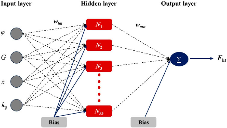
Figure 2. The final structure of the RBF model.

3.2 Multilayer perceptron (MLP)

Similar to the structure of the RBF model, the MPL model is consisted of one input layer, one output layer, and at least one hidden layer. The neuron in each layer is connected by weights (w) and bias (b). The main difference between the MLP and RBF are the way that the neurons process data and the selection of activation function (Hemmati-Sarapardeha et al., 2018; Zendehboudi et al., 2019). The output of the jth neurons in the output layer can be expressed as:

$y_j=f\left({\displaystyle \sum _{i=1}^n}{w}_{ji}{x}_i+b_j\right)(12)$

where y_j denotes the output of the jth neuron in the output layer, f denotes the activation function, n denotes the number of neurons in the hidden layer, w_ji denotes the connection weight between the jth neuron in the hidden layer and the ith neuron in input layer, x_i denotes the output of the ith neuron in the input layer, and b_j denotes the bias of the jth neuron. Based on a comprehensive literature review, the linear function (Purelin) and the tangent sigmoid function (Tansig), respectively, were selected as the activation functions for the output layer and the hidden layer. The expressions of these functions are given as:

$\text{Purelin}:f\left(x\right)=x(13)$

$\text{Tansig}:f\left(x\right)=\frac{e^x-e^{-x}}{e^x+e^{-x}}=\frac{2}{1+e^{-2x}}-1(14)$

In the MLP model, the number of neurons in the input layer is equal to the number of input variables (=4), and the number of neurons in the output layer is equal to the number of output variable (=1). To determine the structure of the MLP model, the Levenberg Marquardt (LM) algorithm was utilized to train the model (Khalifeh and Vaferi, 2019). Meanwhile, the trial-and-error method was utilized to determine the number of neurons in the hidden layer. The optimum values of n, w, and b for the MLP model are tabulated in Supplementary Appendix Table A2. The optimum structure of the MLP model developed in this work was determined as 4–32–1.

3.3 Least‒squares support‒vector machine (LSSVM)

The support vector machine (SVM) was proposed in 1964, and has been widely used in question classification, pattern recognition, and nonlinear regression (Hemmati-Sarapardeh et al., 2020; Huang et al., 2024). With the continuous development of technology, the traditional SVM have expressed frustration in solving the complicated problems with large amount of data samples (Zendehboudi and Saidur, 2018). To overcome this issue, the LSSVM model was developed on the basis of SVM, by adding a regression error in the optimization constraints. In the LSSVM model, the mathematic relation between the input vectors X = {x₁, x₂, …, x_n} (where n is the number of points) and the output vectors Y = {y₁, y₂, …, y_n} can be described by the penalty function. The penalty function can be expressed as follows:

$Q_{\text{LSSVM}}=\frac{1}{2}{w}^{\mathrm{T}}w+\frac{1}{2}\gamma {\displaystyle \sum _{i=1}^n}{e}_i^2(15)$

subjected to the following equality constraints:

$y_i=w^{\mathrm{T}}g\left(x_i\right)+b+e_i,i=1,2,3,\dots ,n(16)$

where T denotes the transpose matrix, γ denotes the summation of regression errors, e_i denotes the regression error between the predicted and actual values, g (x) denotes the mapping function, w denotes the weight, and b denotes the bias.

To solve the aforementioned optimization problems, the corresponding Lagrange function is proposed and can be expressed as (Hemmati-Sarapardeh et al., 2020):

$L\left(w,b,\alpha ,e\right)=\frac{1}{2}{w}^{\mathrm{T}}w+\frac{1}{2}\gamma {\displaystyle \sum _{i=1}^n}{e}_i^2-{\displaystyle \sum _{i=1}^n}{\alpha }_i\left[w^{\mathrm{T}}g\left(x_i\right)+b+e_i-y_i\right](17)$

where α_i denotes the Lagrange multiplier.

By setting the derivatives of w, b, α, and e to zero, an optimal solution to the problem can be obtained as:

$\frac{\partial L\left(w,b,\alpha ,e\right)}{\partial e_i}=0\Rightarrow {\alpha }_i=\gamma \cdot e_i(18)$

$\frac{\partial L\left(w,b,\alpha ,e\right)}{\partial w}=0\Rightarrow w={\displaystyle \sum _{i=1}^n}{\alpha }_{i}g\left(x_i\right)(19)$

The LSSVM model can be expressed as follows:

$y={\displaystyle \sum _{i=1}^n}{\alpha }_i{x}_i^{\mathrm{T}}x+b(20)$

For nonlinear regression problems, the Kernel function is introduced to combine with Eq. 17

$y={\displaystyle \sum _{i=1}^n}{\alpha }_{i}K\left(x_i,x\right)+b(21)$

Owing to the higher accuracy, better convergence and simplicity, the radial basis function (RBF) has been widely used as kernel function in LSSVM which can be given as follows:

$K\left(x_i,x\right)=\exp \left(-\frac{{‖x_i-x‖}^2}{{\sigma }^2}\right),i=1,2,3,\dots ,n(22)$

where σ² denote the bandwidth of the RBF.

The values of the hyper-parameters (σ² and γ) are very important for the performance of LSSVM. According to the cross-validation method, the optimum σ² and γ were determined as 0.2916 and 40.723, respectively.

3.4 Adaptive neuro fuzzy inference system (ANFIS)

The adaptive neuro fuzzy inference system (ANFIS) is a new kind of inference system which combines the artificial neuron network (ANN) and fuzzy logic algorithms (Bahiraei et al., 2019). For a first-order Takagi–Sugeno ANFIS model with two input variables (x₁ and x₂) and one output variable (y), the model can be constructed by the following If–Then rules (Aminossadati et al., 2012):

Rule 1 If x₁ is A₁ and x₂ is B₁ then y₁ = p₁x₁ + q₁x₂ + r₁

Rule 2 If x₁ is A₂ and x₂ is B₂ then y₂ = p₂x₁ + q₂x₂ + r₂

where A_i and B_i denote the fuzzy sets of x₁ and x₂, respectively, p_i, q_i, and r_i denote the designing parameters.

In simple terms, ANFIS is a multilayer network which is consists of five layers: fuzzified layer, rule layer, normalized layer, output layer, and summing layer (Mehrabi et al., 2011). In the first fuzzified layer of the ANFIS, the input variables are fuzzified by the membership function. Next, each neuron is processed by relevant rules and the firing strength of each rule is obtained. In the third layer, the firing strength of each rule is normalized. In the fourth output layer, the output of each rule is obtained by multiplying the normalized value of firing strength. In the final layer, the overall output of the model is determined by the weighted average output of all rules.

By comprehensive considering of the number of samples and the capability of the ANFIS model, the subtractive clustering method (SCM) and the least squares-back propagation algorithm were selected to train and optimize the ANFIS model (Tatar et al., 2016). Through compare and analysis, the Gaussian function and the linear function were selected as the membership function, respectively, for the input layer and the output layer. Meanwhile, the optimum number of membership function, fuzzy rule, linear parameter, and nonlinear parameter were determined as 22, 36, 146, and 48, respectively.

4 Results and discussion

4.1 Accuracy analysis

To comprehensively assess the accuracy of the developed intelligence models, the deviation between the experimental and the predicted values, for the RBF, MLP, LSSVM, and ANFIS, are given in Figure 3, Figure 4, Figure 5, and Figure 6, respectively. In these figures, the red triangle and the yellow circular, respectively, represent the training data and the testing data.

Figure 3

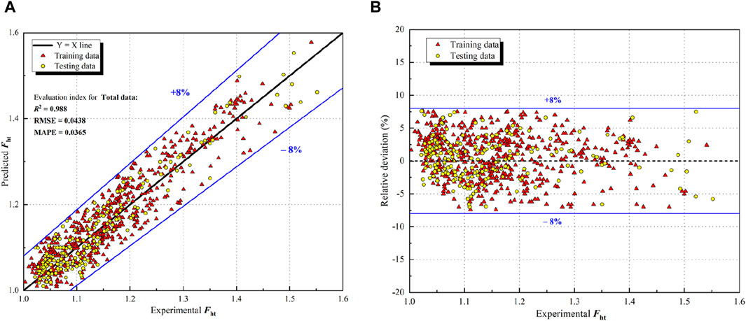
Figure 3. Deviation of the developed RBF models. (A) Cross plot, and (B) Error distribution plot.

Figure 4

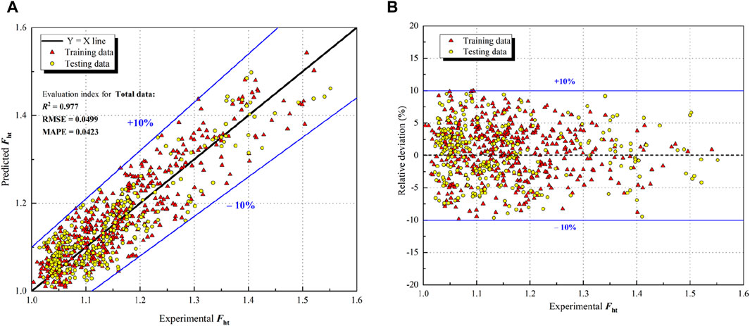
Figure 4. Deviation of the developed MLP models. (A) Cross plot, and (B) Error distribution plot.

Figure 5

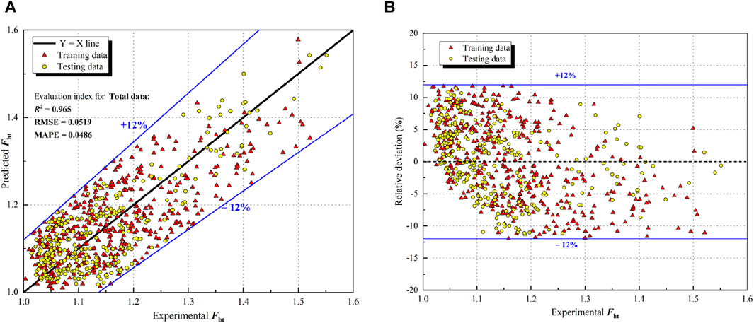
Figure 5. Deviation of the developed LSSVM models. (A) Cross plot, and (B) Error distribution plot.

Figure 6

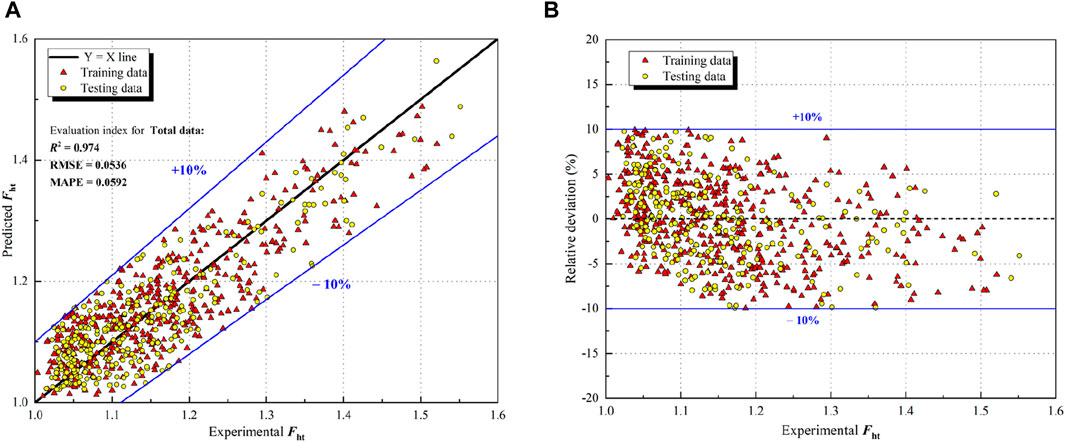
Figure 6. Deviation of the developed ANFIS models. (A) Cross plot, and (B) Error distribution plot.

As shown from Figure 3–6, the deviation for the RBF, MLP, LSSVM, and ANFIS were within the range of ±8%, ±10%, ±12%, and ±10.3%, respectively. For the training data, the prediction errors by the RBF, MLP, LSSVM, and ANFIS were −7.42%–7.56%, −9.86%–9.92%, −11.96%–11.81%, and −9.94%–9.93%, respectively. While for the testing data, the prediction errors were −7.06%–7.68%, −9.65%–9.50%, −11.33%–11.42%, and −9.91%–9.76%, respectively. It can be seen that the accuracies of the developed intelligence models can meet the requirements of industrial application.

To further quantification and comparison of the accuracy of the intelligence models, the performance parameters of the intelligence models and the empirical correlations, were tabulated in Table 4.

Table 4

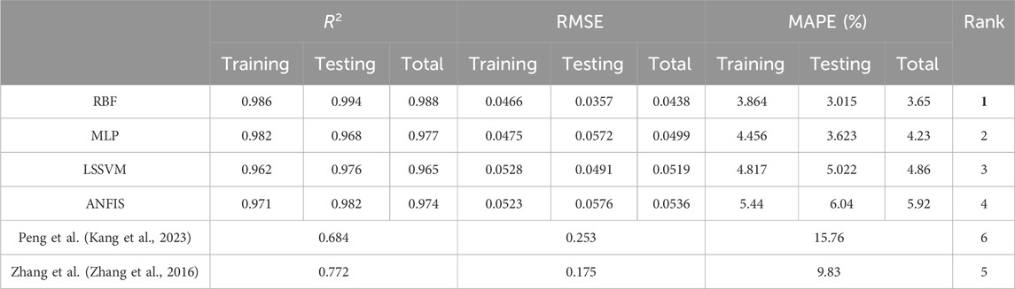
Table 4. Performance parameters of the developed intelligence models.

As can be clearly seen from Table 4, the highest value of R² and the lowest values of RMSE and MAPE were found in the RBF model. The performance of the RBF model was superior than those of other models. Meanwhile, the intelligence models exhibited better performances than the empirical correlations significantly, with much lower RMSE and MAPE values. This was mainly because the empirical correlations were derived based on the common regression techniques and limited experimental data. In rank order of best to worst, the accuracies of the model were: RBF > MLP >; LSSVM > ANFIS > Zhang’s > Peng’s.

4.2 Variation trend analysis

The accuracy of the developed RBF model has been confirmed. In order to check whether the RBF model could predict the variation trend of the output (F_ht) with the inputs (φ, G, x, and k_p), a comprehensive variation trend analysis was conducted. Variations of the F_ht with φ, G, x, and k_p are presented in Figure 7, Figure 8, and Figure 9, respectively. In these figures, the scatter symbols represent the experimental results, and the solid line represent the predicted ones by the RBF model, respectively.

Figure 7

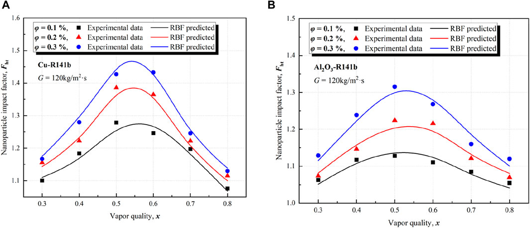
Figure 7. Variations of the nanoparticle impact factor (F_ht) with respect to the vapor quality (x) under different nanoparticle concentration (φ) using: (A) Cu‒R141b, and (B) Al₂O₃‒R141b.

Figure 8

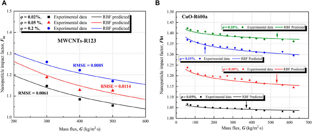
Figure 8. Variations of the nanoparticle impact factor (F_ht) with respect to the mass flux (G) under different nanoparticle concentration (φ) using: (A) MWCNTs‒R123, and (B) CuO‒R600a.

Figure 9

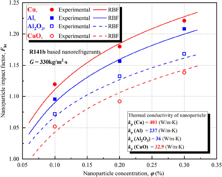
Figure 9. Variations of the nanoparticle impact factor (F_ht) with respect to the nanoparticle concentration (φ) for the R141b based nanorefrigerant containing Cu, Al, CuO, and Al₂O₃ nanoparticles.

Figure 7A,B shows the variations of the F_ht with respect to the vapor quality (x) under different nanoparticle concentration (φ), respectively, for Cu‒R141b nanorefrigerant and Al₂O₃‒R141b nanorefrigerant. As can be seen in Figure 7 that the variation trends of the F_ht with x and φ, predicted by the RBF model, were in consistency with the experimental observation. For a given nanoparticle concentration, F_ht increased firstly, continuously came up to a “peak value”, and then decreased as the vapor quality (x) increased. A similar phenomenon was observed in the experiment researches by Akhavan‒Behabadi et al. (Akhavan-Behabadi et al., 2014) and Zhang et al. (Zhang et al., 2016). This can be attributed to the fact that the nanoparticles during flow boiling significantly promoted the flow pattern toward the annular flow regime at the middle vapor quality. With further increasing vapor quality, the liquid content of refrigerant decreased and the annular flow regime disappeared, thereby deteriorating the heat transfer coefficient. For Cu‒R141b nanorefrigerant, the RMSE between the experimental F_ht and predicted ones for φ = 0.1%, 0.2%, and 0.3%, respectively, were 0.006, 0.0141, and 0.009. For Al₂O₃‒R141b nanorefrigerant, the RMSE between the experimental F_ht and predicted ones for φ = 0.1%, 0.2%, and 0.3%, respectively, were 0.0072, 0.0094, and 0.02311.

Figure 8A,B shows the variations of the F_ht with respect to the mass flux (G) under different nanoparticle concentration (φ), respectively, for MWCNTs‒R123 and CuO‒R600a nanorefrigerants. The predicted variation trends of the F_ht with G and φ, predicted by the RBF model, were consistent with the experimental observation. The nanoparticle impact factor F_ht decreased with increasing mass flux for a given nanoparticle concentration. This can be explained by the fact the heat transfer enhancement can be induced by increasing mass flux, while the contribution of nanoparticle to the heat transfer enhancement is gradually inhibited with the increase of mass flux (Peng et al., 2009; Sun and Yang, 2013).

In Figure 9, the variation trends of the F_ht with φ, predicted by the RBF model, were consistent with the experimental observation. The HTC of the nanorefrigerant increased with the increase of the thermal conductivity of nanoparticle. For Cu‒R141b, Al‒R141b, Al₂O₃‒R141b, and Cu‒R141b nanorefrigerants, the RMSEs between the experimental F_ht and predicted ones, respectively, were 0.0166, 0.0145, 0.0134, and 0.0172.

In order to quantitative investigate the error distribution of the RBF model with the variations of different types of inputs, the deviation distribution of the present RBF model in different ranges of φ, G, x, and k_p are, respectively, given in Figure 10A–D. In this figure, the red bars represent the values of RMSE, and the blue bars represent the values of MAPE. As can be seen from Figure 10 that the error distributions by the RBF model were relatively uniform in different ranges of φ, G, x, and k_p, while no obvious local error aggregation was found. Therefore, it is demonstrated that the RBF model can effectively predict the variation trend of the output (F_ht) with the inputs (φ, G, x, and k_p).

Figure 10

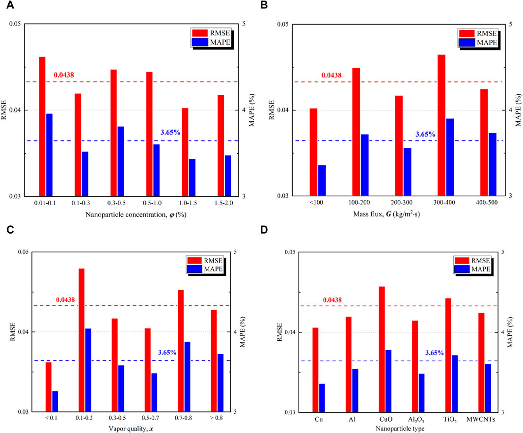
Figure 10. The error distribution of the RBF model in different ranges of. (A) nanoparticle concentration, (B) mass flux, (C) vapor quality, and (D) nanoparticle’s thermal conductivity.

To now, the developed RBF model was proven to be a favorable tool for predicting the flow boiling HTC of nanorefrigerant in many common experimental conditions and practical scenarios, based on the results given in Figure 3-10.

4.3 Sensitivity analysis

To promote the application of nanorefrigerant, a thorough understanding on the impact degree of each input variable (φ, G, x, and k_p) on the output (F_ht) is essential. For this purpose, a sensitivity analysis was carried out using the correlation proposed by Pearson (Mohagheghian et al., 2015). The Pearson’s correlation has been widely used for sensitivity analysis in the existing literature and can be expressed as (Khalifeh and Vaferi, 2019):

$r\left(\text{in}{p}_k,F_{\text{ht}}\right)=\frac{{\displaystyle \sum _{i=1}^n}\left(\text{in}{p}_{k,i}-\overline{\text{in}{p}_k}\right)\left({F_{\text{ht}}}_{,i}-\overline{F_{\text{ht}}}\right)}{\sqrt{{{\displaystyle \sum _{i=1}^n}\left(\text{in}{p}_{k,i}-\overline{\text{in}{p}_k}\right)}^2{\left({F_{\text{ht}}}_{,i}-\overline{F_{\text{ht}}}\right)}^2}}(23)$

where, r denotes the relevancy factor, which ranged between −1 and +1; inp_k,i denotes the ith value of the kth input variable; $\overline{\text{in}{p}_k}$ denote the average value of the kth input variable; F_{ht, i} denote the ith value of the output, and $\overline{F_{\text{ht}}}$ denote the average value of the output. It is worth mentioning that the sign of r directly reflects the proportional relation between the output variable and the input variables. In simple term, a positive r indicated that the relation between the input variable and output variable is proportional, whereas a negative r indicated that the proportional between the input and output is inversely. Meanwhile, the larger the absolute value of r is, the greater the impact degree of input variable on output is.

According to Eq. 23, the relevancy factor of each input variable on the output are presented in Figure 11.

Figure 11

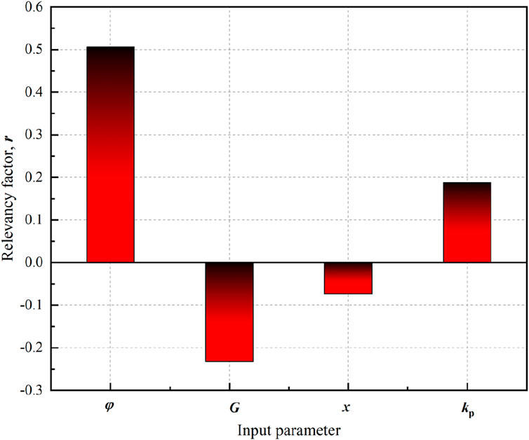
Figure 11. The relevancy factor of each input variable on the output.

As can be seen from Figure 11 that the impact degrees of all input variables in decreasing order are: |r|(φ) = 0.506, |r|(G) = 0.232, |r|(k_p) = 0.188, and |r|(x) = 0.074. Among all the input variables, the nanoparticle concentration (φ) has the greatest impact degree on the output. Meanwhile, the r values for φ and k_p were positive, which indicated that the increase of φ and k_p resulted in the increase of F_ht. On the other hand, the r values for G and x were negative, which indicated that the increase of G and x resulted in the decrease of F_ht. The above results are consistent with the results of previous variation trend analysis.

5 Conclusion

In order to explore the feasibility of employing the nanorefrigerant in the ORC and IES, four intelligence models—RBF, MLP, LSSVM, and ANFIS—for predicting the flow boiling heat transfer coefficient of the nanorefrigerants, were developed based on 765 experimental data samples. The comprehensive performances of the models were analyzed in detail, including accuracy, physical variation trend, and sensitivity. The following conclusions were drawn from the study:

(1) The predicted values by the RBF, MLP, LSSVM, and ANFIS were in good agreement with the experimental values. According to the comprehensive statical analysis (R², RMSE, and MAPE) for the training, testing and total dataset, the RBF model was superior than those of other intelligence models and the existing empirical models in predicting the flow boiling heat transfer coefficient of nanorefrigerants.

(2) According to the variation trend analysis, the RBF model accurately captured the variation trend of the output (F_ht) with the inputs (φ, G, x, and k_p). F_ht increases with increasing φ and k_p, while decrease with G and x.

(3) The impact degrees of all input variables in decreasing order were nanoparticle concentration (φ), mass flux (G), thermal conductivity of nanoparticle (k_p), and vapor quality (x).

Data availability statement

The original contributions presented in the study are included in the article/Supplementary Material, further inquiries can be directed to the corresponding authors.

Author contributions

SZ: Conceptualization, Funding acquisition, Investigation, Methodology, Validation, Writing–original draft, Writing–review and editing. YL: Data curation, Supervision, Writing–review and editing. ZX: Resources, Software, Writing–review and editing. LM: Formal Analysis, Investigation, Resources, Writing–review and editing. YL: Data curation, Methodology, Supervision, Validation, Writing–original draft.

Funding

The author(s) declare that financial support was received for the research, authorship, and/or publication of this article. This work was supported by the Talent Support Plan of Yunnan Province (XDYC‒QNRC‒2022‒0122), and Scientific Research Foundation of Kunming Metallurgy College [Xxrcxm201802].

Conflict of interest

The authors declare that the research was conducted in the absence of any commercial or financial relationships that could be construed as a potential conflict of interest.

Publisher’s note

All claims expressed in this article are solely those of the authors and do not necessarily represent those of their affiliated organizations, or those of the publisher, the editors and the reviewers. Any product that may be evaluated in this article, or claim that may be made by its manufacturer, is not guaranteed or endorsed by the publisher.

Supplementary material

The Supplementary Material for this article can be found online at: https://www.frontiersin.org/articles/10.3389/fenrg.2024.1412538/full#supplementary-material

References

Akhavan-Behabadi, M. A., Nasr, M., and Baqeri, S. (2014). Experimental investigation of flow boiling heat transfer of R-600a/oil/CuO in a plain horizontal tube. Exp. Therm. Fluid Sci. 58, 105–111. doi:10.1016/j.expthermflusci.2014.06.013

CrossRef Full Text | Google Scholar

Aminossadati, S., Kargar, A., and Ghasemi, B. (2012). Adaptive network based fuzzy inference system analysis of mixed convection in a two-sided lid-driven cavity filled with a nanofluid. Int. J. Therm. Sci. 52, 102–111. doi:10.1016/j.ijthermalsci.2011.09.004

CrossRef Full Text | Google Scholar

Bahiraei, M., Heshmatian, S., and Moayedi, H. (2019). Artificial intelligence in the field of nanofluids: a review on applications and potential future directions. Powder Technol. 353, 276–301. doi:10.1016/j.powtec.2019.05.034

CrossRef Full Text | Google Scholar

Baqeri, S., Akhavan-Behabadi, M. A., and Ghadimi, B. (2014). Experimental investigation of the forced convective boiling heat transfer of R-600a/oil/nanoparticle. Int. Commun. Heat Mass Transf. 55, 71–76. doi:10.1016/j.icheatmasstransfer.2014.04.005

CrossRef Full Text | Google Scholar

Choi, S. U. S., and Eastman, J. A. (1995). “Enhancing thermal conductivity of fluids with nanoparticles,” in Presented at International Mechanical Engineering Congress and Exhibition, San Francisco, CA, November 1995.

Google Scholar

Dadhich, M., Prajapati, O. S., and Rohatgi, N. (2020). Flow boiling heat transfer analysis of Al2O3 and TiO2 nanofluids in horizontal tube using artificial neural network (ANN). J. Therm. Analysis Calorim. 139, 3197–3217. doi:10.1007/s10973-019-08674-y

CrossRef Full Text | Google Scholar

Dey, P., and Mandal, B. K. (2021). Performance enhancement of a shell-and-tube evaporator using Al2O3/R600a nanorefrigerant. Int. J. Heat Mass Transf. 170, 121015. doi:10.1016/j.ijheatmasstransfer.2021.121015

CrossRef Full Text | Google Scholar

Fahliyany, H. G., Ansari, S., Mohammadi, M., Jafari, S., Schaffie, M., Ghaedi, M., et al. (2024). Toward predicting thermal conductivity of hybrid nanofluids: application of a committee of robust neural networks, theoretical, and empirical models. Powder Technol. 437, 119506. doi:10.1016/j.powtec.2024.119506

CrossRef Full Text | Google Scholar

Feng, Y. Q., Zhang, Q., Liu, Y. Z., Liang, H. j., Lu, Y. y., He, Z. x., et al. (2024). Experimental investigation on stability and evaluation of nanorefrigerant applied on organic Rankine cycle system. Appl. Therm. Eng. 336, 121683. doi:10.1016/j.applthermaleng.2023.121683

CrossRef Full Text | Google Scholar

Hemmati-Sarapardeh, A., Varamesh, A., Amar, M. N., Husein, M. M., and Dong, M. (2020). On the evaluation of thermal conductivity of nanofluids using advanced intelligent models. Int. Commun. Heat Mass Transf. 118, 104825. doi:10.1016/j.icheatmasstransfer.2020.104825

CrossRef Full Text | Google Scholar

Hemmati-Sarapardeha, A., Varamesh, A., Huseinc, M. M., and Karan, K. (2018). On the evaluation of the viscosity of nanofluid systems: modeling and data assessment. Renew. Sustain. Energy Rev. 81, 313–329. doi:10.1016/j.rser.2017.07.049

CrossRef Full Text | Google Scholar

Henderson, K., Park, Y.-G., Liu, L. P., and Jacobi, A. M. (2010). Flow-boiling heat transfer of R-134a-based nanofluids in a horizontal tube. Int. J. Heat Mass Transf. 53, 944–951. doi:10.1016/j.ijheatmasstransfer.2009.11.026

CrossRef Full Text | Google Scholar

Huang, H. Y., Li, C. Q., Huang, S. Y., and Shang, Y. (2024). A sensitivity analysis on thermal conductivity of Al2O3-H2O nanofluid: a case based on molecular dynamics and support vector regression method. J. Mol. Liq. 393, 123652. doi:10.1016/j.molliq.2023.123652

CrossRef Full Text | Google Scholar

Jamei, M., Pourrajab, R., Ahmadianfar, I., and Noghrehabadi, A. (2020). Accurate prediction of thermal conductivity of ethylene glycol-based hybrid nanofluids using artificial intelligence techniques. Int. Commun. Heat Mass Transf. 116, 104624. doi:10.1016/j.icheatmasstransfer.2020.104624

CrossRef Full Text | Google Scholar

Kang, L., Wang, J., Yuan, X., Cao, Z., Yang, Y., Deng, S., et al. (2023). Research on energy management of integrated energy system coupled with organic Rankine cycle and power to gas. Energy Convers. Manag. 287, 117117. doi:10.1016/j.enconman.2023.117117

CrossRef Full Text | Google Scholar

Kanti, P., Sharma, K. V., Yashawantha, K. M., Jamei, M., and Said, Z. (2022). Properties of water-based fly ash-copper hybrid nanofluid for solar energy applications: application of RBF model. Sol. Energy Mater. Sol. Cells 234, 111423. doi:10.1016/j.solmat.2021.111423

CrossRef Full Text | Google Scholar

Khalifeh, A., and Vaferi, B. (2019). Intelligent assessment of effect of aggregation on thermal conductivity of nanofluids—comparison by experimental data and empirical correlations. Thermochima Acta 681, 178377. doi:10.1016/j.tca.2019.178377

CrossRef Full Text | Google Scholar

Kosmadakis, G., and Neofytou, P. (2020). Investigating the performance and cost effects of nanorefrigerants in a low-temperature ORC unit for waste heat recovery. Energy 204, 117966. doi:10.1016/j.energy.2020.117966

CrossRef Full Text | Google Scholar

Kumar, A., Gupta, P. R., Tiwari, A. K., and Said, Z. (2022). Performance evaluation of small scale solar organic Rankine cycle using MWCNT + R141b nanorefrigerant. Energy Convers. Manag. 260, 115631. doi:10.1016/j.enconman.2022.115631

CrossRef Full Text | Google Scholar

Kumar, R., Singh, D. S., and Chander, S. (2024). Experimental investigation and correlation development of flow condensation with R123/MWCNTs nanorefrigerant inside a horizontal tube. Int. J. Therm. Sci. 197, 108811. doi:10.1016/j.ijthermalsci.2023.108811

CrossRef Full Text | Google Scholar

Mehrabi, M., Pesteei, S., and Pashaee, T. (2011). Modeling of heat transfer and fluid flow characteristics of helicoidal double-pipe heat exchangers using Adaptive Neuro-Fuzzy Inference System (ANFIS). Int. Commun. Heat Mass Transf. 38, 525–532. doi:10.1016/j.icheatmasstransfer.2010.12.025

CrossRef Full Text | Google Scholar

Mohagheghian, E., Zafarian‒Rigaki, H., Ghahfarrokhi, Y. M., and Hemmati-Sarapardeh, A. (2015). Using an artificial neural network to predict carbon dioxide compressibility factor at high pressure and temperature. Korean J. Chem. Eng. 32 (10), 2087–2096. doi:10.1007/s11814-015-0025-y

CrossRef Full Text | Google Scholar

Ngangu’e, M., Lekan´e, N. N., Njock, J. P., Sosso, O. T., and Stouffs, P. (2023). Working fluid selection for a high efficiency integrated power/cooling system combining an organic Rankine cycle and vapor compression-absorption cycles. Energy 277, 127709. doi:10.1016/j.energy.2023.127709

CrossRef Full Text | Google Scholar

Peng, H., Ding, G. L., Jiang, W. T., Hu, H., and Gao, Y. (2009). Heat transfer characteristics of refrigerant-based nanofluid flow boiling inside a horizontal smooth tube. Int. J. Refrig. 32 (6), 1259–1270. doi:10.1016/j.ijrefrig.2009.01.025

CrossRef Full Text | Google Scholar

Said, Z., Rahman, S. M. A., Sohail, M. A., and B S, B. (2023). Analysis of thermophysical properties and performance of nanorefrigerants and nanolubricant-refrigerant mixtures in refrigeration systems. Case Stud. Therm. Eng. 49, 103274. doi:10.1016/j.csite.2023.103274

CrossRef Full Text | Google Scholar

Sheikholeslami, M., Rezaeianjouybari, B., Darzi, M., Shafee, A., Li, Z., and Nguyen, T. K. (2019). Application of nano-refrigerant for boiling heat transfer enhancement employing an experimental study. Int. J. Heat Mass Transf. 14, 974–980. doi:10.1016/j.ijheatmasstransfer.2019.07.043

CrossRef Full Text | Google Scholar

Sun, B., and Yang, D. (2013). Experimental study on the heat transfer characteristics of nanorefrigerants in an internal thread copper tube. Int. J. Heat Mass Transf. 64, 559–566. doi:10.1016/j.ijheatmasstransfer.2013.04.031

CrossRef Full Text | Google Scholar

Sun, B., and Yang, D. (2014). Flow boiling heat transfer characteristics of nano-refrigerants in a horizontal tube. Int. J. Refrig. 38 (1), 206–214. doi:10.1016/j.ijrefrig.2013.08.020

CrossRef Full Text | Google Scholar

Tatar, A., Barati-Harooni, A., Najaf-Marghmaleki, A., Norouzi-Farimani, B., and Mohammadi, A. H. (2016). Predictive model based on ANFIS for estimation of thermal conductivity of carbon dioxide. J. Mol. Liq. 224, 1266–1274. doi:10.1016/j.molliq.2016.10.112

CrossRef Full Text | Google Scholar

Tazarv, S., Saffar-Avval, M., Khalvati, F., Mirzaee, E., and Mansoori, Z. (2016). Experimental investigation of saturated flow boiling heat transfer to TiO2/r141b nanorefrigerant. Exp. Heat. Transf. 29, 188–204. doi:10.1080/08916152.2014.973976

CrossRef Full Text | Google Scholar

Yang, D., Sun, B., Li, H. W., and Fan, X. (2015). Experimental study on the heat transfer and flow characteristics of nanorefrigerants inside a corrugated tube. Int. J. Refrig. 56, 213–223. doi:10.1016/j.ijrefrig.2015.04.011

CrossRef Full Text | Google Scholar

Yilmaz, M., Cimsit, C., Keven, A., and Karaali, R. (2024). Analysis of cascade vapor compression refrigeration system using nanorefrigerants: energy, exergy, and environmental (3E). Case Stud. Therm. Eng. 57, 104373. doi:10.1016/j.csite.2024.104373

CrossRef Full Text | Google Scholar

Yu, L., Lai, K. K., and Wang, S. (2008). Multistage RBF neural network ensemble learning for exchange rates forecasting. Neurocomputing 71, 3295–3302. doi:10.1016/j.neucom.2008.04.029

CrossRef Full Text | Google Scholar

Zarei, M. J., Ansari, H. R., Keshavarz, P., and Zerafat, M. M. (2020). Prediction of pool boiling heat transfer coefficient for various nano-refrigerants utilizing artificial neural networks. J. Therm. analysis Calorim. 139, 3757–3768. doi:10.1007/s10973-019-08746-z

CrossRef Full Text | Google Scholar

Zendehboudi, A., and Saidur, R. (2018). A reliable model to estimate the effective thermal conductivity of nanofluids. Heat Mass Transf. 55 (2), 397–411. doi:10.1007/s00231-018-2420-5

CrossRef Full Text | Google Scholar

Zendehboudi, A., Saidur, R., Mahbubul, I. M., and Hosseini, S. (2019). Data-driven methods for estimating the effective thermal conductivity of nanofluids: a comprehensive review. Int. J. Heat Mass Transf. 131, 1211–1231. doi:10.1016/j.ijheatmasstransfer.2018.11.053

CrossRef Full Text | Google Scholar

Zhang, S., Ge, Z., Wang, H., and Wang, H. (2016). Characteristics of flow boiling heat transfer and pressure drop of MWCNT–R123 nanorefrigerant: experimental investigations and correlations. Nanoscale Microscale Thermophys. Eng. 20, 97–120. doi:10.1080/15567265.2016.1208693

CrossRef Full Text | Google Scholar