Data-driven industrial park microgrids robust optimization method

In order to accurately describe the impact of the volatility and randomness of renewable energy output power on the operation of industrial park microgrids, a data-driven robust optimization method for industrial park microgrids is proposed. Firstly, based on the traditional interval set, the uncertain parameters of renewable energy output are modeled using a polyhedral set. Then, an ellipsoidal uncertainty set is established using historical data of renewable energy output. By connecting high-dimensional ellipsoidal vertices, a data-driven convex hull polyhedron set is established. Then, the uncertain parameters are better enveloped by scaling the convex hull set. A data-driven robust optimization model for industrial park microgrid was further established, and the column and constraint (C&CG) generation algorithm was used to solve the model. Finally, simulation comparisons were conducted through examples, and the results showed that the data-driven industrial park microgrids robust optimization method can reduce conservatism and improve the robustness of optimization results, demonstrating the effectiveness of the proposed method.

1 Introduction

With the increasingly prominent environmental and climate issues caused by excessive reliance on traditional fossil fuels, accelerating energy transition and sustainable development on a global scale has become a widely accepted consensus (Farh et al., 2024). To address the challenges of energy supply diversity and the intermittency of renewable energy sources, the industrial park microgrids featuring complementary and coupled forms of multiple energy supplies has emerged (Ishaq and Dincer, 2024). However, due to the instability of renewable energy outputs, power generation is affected by various factors such as climate, weather, and seasons, leading to significant fluctuations in power supply. These fluctuations can potentially trigger instability or even collapse of the industrial park microgrids, posing significant challenges to its safety and stability (Poodeh et al., 2025).

Existing research on the industrial park microgrids operation planning focuses on energy utilization efficiency and enhancing system stability. For instance, in Arooj (2024), system stability is improved by adopting demand-side response under the premise of considering flexible resources. In Rezazadeh and Avami (2024), a comprehensive energy system with detailed power-to-gas conversion and carbon cycling is established through the utilization of the carbon trading market. In Rahman et al. (2025), the grid partitioning of the integrated energy system is optimized by taking into account the characteristics of the load, thereby achieving cost reduction. Synthesizing these studies, there is a noticeable lack of consideration given to the uncertainty of renewable energy output.

To address the issue of uncertainty in renewable energy output, existing uncertainty optimization methods are mainly categorized into two types: stochastic optimization methods (Davidsdottir et al., 2024; Son and Kim, 2024; Aliasghar et al., 2022) and robust optimization methods (Vulusala and Madichetty, 2018; Stewart and Bingham, 2016). Robust optimization methods typically use a set-based approach to describe the distribution range of uncertain parameters. Unlike stochastic methods, robust optimization does not require the probability distribution of uncertain parameters and avoids the high-dimensional problems introduced by numerous scenarios. Consequently, it has gained increasing attention in the optimal operation of industrial park microgrids.

To enhance the reliability of robust optimization results and describe the correlations among uncertain parameters, recent studies have employed historical data of uncertain variables to explore the relationships between the variations of random variables, leading to the proposal of data-driven uncertainty sets (Sulaiman et al., 2024; Freitas et al., 2007; Ibraheemi and Janabi, 2024). For instance (Zhang et al., 2024a), constructed the uncertainty of photovoltaic power generation using historical data from smart meters and phasor measurement units to solve the problem of voltage regulation (Zhang et al., 2024b). constructed an uncertainty set using historical vehicle travel data to analyze the impact of large-scale transportation electrification on power systems (Lorca and Sun, 2015). established a polyhedral uncertainty set based on historical wind power data for economic dispatch modeling, analysis, and optimization (Jalilvand-Nejad et al., 2016). Proposed a correlated polyhedral uncertainty set model by bending the boundaries of a polyhedral set through mathematical analysis, building on the polyhedral set approach (Hamed and Rasoul, 2021). further refined the approach of Jalilvand-Nejad et al. (2016) by constructing a generalized correlated polyhedral uncertainty set model, allowing the polyhedral set to better envelop the range of uncertain parameters (Degefa et al., 2015). Constructed an ellipsoidal set to describe photovoltaic (PV) output and proposed an affine adjustable robust optimization strategy for active distribution networks. Although the ellipsoidal set effectively considers the correlations among uncertain parameters, its nonlinear structure increases the difficulty of solving the model. While Lorca and Sun (2015), Jalilvand-Nejad et al. (2016), Hamed and Rasoul (2021), and Degefa et al. (2015) consider the correlations within the uncertainty sets, the broader coverage of the uncertainty sets they establish can lead to increased conservatism in decision-making.

In addition to polyhedral and ellipsoidal sets, another common method is constructing uncertainty sets based on extreme scenarios. In Moradian et al. (2024) and Akter et al. (2025), historical data is first selected to form the uncertainty set. Then, extreme scenarios are identified based on the historical data, and convex hull sets are constructed from these scenarios. An appropriate scaling factor is introduced to cover all historical data, and finally, a robust optimization model based on extreme scenarios is established. The method in Ayene and Yibre (2024) and Bifei et al. (2022) does not predefine the shape of the uncertainty set but represents it as the convex hull of historical scenarios. These studies have made improvements regarding the conservativeness of polyhedral sets. However, although the uncertainty sets based on extreme scenarios can address the conservatism issue, they have a large number of vertices, making them difficult to solve. Therefore, this paper proposes a data-driven convex hull uncertainty set model. This model can not only reduce the conservatism of the solution but also decrease the difficulty of solving.

Against this research backdrop, considering the lack of attention to uncertain energy inputs in industrial park microgrids, this paper proposes a data-driven robust optimization method for industrial park microgrids. First, traditional polyhedral set modeling is conducted based on interval sets. Then, ellipsoidal sets are constructed based on historical scenarios, and the vertices of the ellipsoids are connected to form convex hull polyhedral sets. Finally, the constructed convex hull set is scaled to cover all historical scenarios. Furthermore, the data-driven convex hull model is embedded into the robust optimization model of the industrial park microgrids. The effectiveness of iu-the proposed method is verified through a case study of an integrated energy system in a specific region.

This paper will mainly make contributions in the following aspects:

1. In view of the current situation that the integrated energy system insufficiently considers the injection of uncertain energy sources, a data-driven robust optimization method for industrial park microgrids is proposed.

2. Aiming at the deficiencies of traditional uncertain set modeling, traditional polyhedron set modeling is first carried out on the interval set. Then, an elliptical set is constructed based on historical scenarios. Subsequently, the vertices of the ellipse are connected to construct a convex hull polyhedron set, and all historical scenarios are covered by scaling, thus establishing a unique data-driven modeling method.

3. The well-constructed data-driven convex hull set model is successfully embedded into the robust optimization model of the industrial park microgrids. Moreover, with the help of an example of an industrial park microgrid in a certain region, the effectiveness of the proposed method is verified.

The rest of this article is organized as follows: Section 2 introduces the different uncertain set modeling. The industrial park microgrid optimization model is introduced in Section 3. In Section 4, the specific objective function and constraints is presented. Section 5 studies the robust optimization method for microgrid in industrial park. Finally, Section 6 concludes.

2 Uncertain set modeling

2.1 Traditional uncertain set modeling

In this paper, the budget uncertainty set U is used to express the range of fluctuations in the magnitude of PV as well as wind power output. The specific expression is shown in Equation 1:

$\mathit{U}=\left\{\begin{array}{l}\mathit{u}=\left[{\stackrel{\sim }{P}}_t^{\text{PV}},{\stackrel{\sim }{P}}_t^{\text{WT}}\right]\\ \mathit{z}=\left[z_t^{\text{PV}},z_t^{\text{WT}}\right]\\ {\stackrel{\sim }{P}}_t^{\text{PV}}=P_t^{\text{PV},\mathrm{f}}+\Delta P^{\text{PV},\max }{z}_t^{\text{PV}}\\ {\stackrel{\sim }{P}}_t^{\text{WT}}=P_t^{\text{WT},\mathrm{f}}+\Delta P^{\text{WT},\max }{z}_t^{\text{WT}}\end{array}\right.(1)$

where ${\stackrel{\sim }{P}}_t^{\text{PV}}$ and ${\stackrel{\sim }{P}}_t^{\text{WT}}$ denote the actual magnitude of output at the moment t for PV and wind power, respectively; $z_t^{\text{PV}}$ and $z_t^{\text{WT}}$ represent the actual output levels of PV and wind power generation at the moment t respectively. $P_t^{\text{PV},\mathrm{f}}$ and $P_t^{\text{WT},\mathrm{f}}$ represent the predicted power output levels of PV and wind energy at the moment t respectively; $\Delta P^{\text{PV},\max }$ and $\Delta P^{\text{WT},\max }$ denote the maximum fluctuation values of PV and wind power generation, respectively; $\mathit{u}$ represents the vector set of PV and wind power output; $\mathit{z}$ stands for the vector set of uncertain variables in PV and wind power generation.

When there is no spatiotemporal correlation between uncertain variables, to better represent the range of variation of uncertain variables, this paper first characterizes them using traditional box sets and polyhedral sets, as shown below.

2.1.1 Box set

The specific expression for a box set can be given as:

$\mathit{U}=\left\{\mathit{z}\in {\mathit{R}}^{N\times 1}|\beta {\mathit{z}}_{\text{down}}\le \mathit{z}\le \beta {\mathit{z}}_{\text{up}}\right\}(2)$

where ${\mathit{R}}^{N\times 1}$ represents the dimension of the uncertain variable; ${\mathit{z}}_{\text{down}}$ and ${\mathit{z}}_{\text{up}}$ represent the maximum and minimum values of the uncertain variables, with values set to 1 and −1, respectively; $\beta$, which is the adjustment coefficient used to regulate the conservativeness of the uncertain set, is set to $\left(0,1\right]$.

From Equation 2, it can be seen that the box set is merely an interval representation of the uncertain variable, and under normal circumstances, the values are often taken at the boundaries. However, since the extreme conditions corresponding to the boundary values have a lower probability of occurrence, the box set fails to accurately represent most other cases. Therefore, a polyhedral set is often required.

2.1.2 Polyhedral set

The specific expression is shown in Equation 3:

$\mathit{U}=\left\{\mathit{z}\in {\mathit{R}}^{N\times 1}\left|\begin{array}{l}\beta {\mathit{z}}_{\text{down}}\le \mathit{z}\le \beta {\mathit{z}}_{\text{up}}\\ {\displaystyle \sum _i^N}{z}_i\le \mathrm{\Gamma }\end{array}\right.\right\}(3)$

where $\mathrm{\Gamma }$ represents the uncertainty of the polyhedral set of uncertain variables, used to constrain the range of uncertainty of the polyhedral set. When the uncertain variables are two-dimensional, the envelope ranges of the polyhedral sets corresponding to different matrices $\mathrm{\Gamma }$ are illustrated as shown in Figure 1.

Figure 1

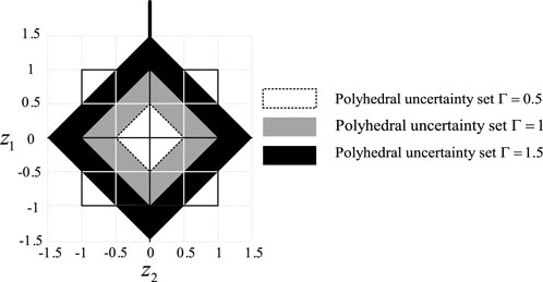
Figure 1. The impact of uncertainty on polyhedral sets.

2.2 Data-driven modeling of uncertain set

When there is spatiotemporal correlation among uncertain parameters, envelope lines can be adopted to represent different sets based on the scatter plots formed by the historical data of uncertain renewable energy output. Figure 2 illustrates the difference in envelope ranges when using box sets and ellipsoid sets.

Figure 2

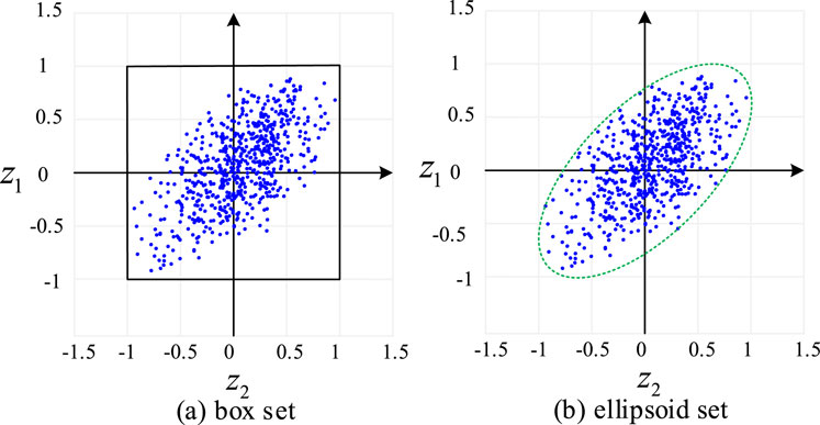
Figure 2. The envelope range of an uncertain set. (a) Box set. (b) Ellipsoid set.

As can be seen in Figure 2a, the box set envelopes all possible outcomes of distributed PV and wind power generation. However, due to the inherent spatiotemporal correlation of distributed PV at different times and locations, the PV output data predominantly clusters around the y = x and y = −x function lines. In this scenario, using a box set to describe the uncertainty of PV output may lead to overly conservative optimization solutions, since the box set not only encompasses all possible fluctuations but also covers areas with low probability of occurrence, which are essentially blank spaces. Therefore, it is necessary to adopt a more suitable modeling approach for uncertain sets.

2.2.1 Ellipsoid set

The specific expression is shown in Equation 4:

$\mathit{U}=\left\{\mathit{z}\in {\mathit{R}}^{N\times 1}|{\left(\mathit{z}-\mathit{c}\right)}^{\mathrm{T}}{\mathit{\Sigma }}^{-1}\left(\mathit{z}-\mathit{c}\right)\le 1\right\}(4)$

where $\mathit{c}$ represents the center point of a high-dimensional ellipsoid, while $\mathrm{\Sigma }\in {\mathit{R}}^{N\times N}$ is a positive definite matrix indicating the offset direction of the high-dimensional ellipsoid relative to the coordinate axes.

As illustrated in Figure 2b, the ellipsoid set, similar to the box set, envelopes all possible outcomes of distributed power generation. Unlike the box set, however, the ellipsoid set reduces the envelopment of blank areas with low probability of fluctuation occurrence, thereby decreasing the conservativeness of the decision results. However, due to the quadratic form of the ellipsoid set’s expression, it introduces complexity in the robust optimization process, increasing the difficulty of the solution.

2.2.2 Generalized convex hull set

Building upon this (Moradian et al., 2024), proposed a generalized convex hull set, which not only effectively reduces the conservativeness of optimization outcomes but also avoids the introduction of quadratic forms during the modeling process. Thus, based on Moradian et al. (2024), this paper constructs a data-driven uncertain set, with the modeling process illustrated in Figure 3.

Figure 3

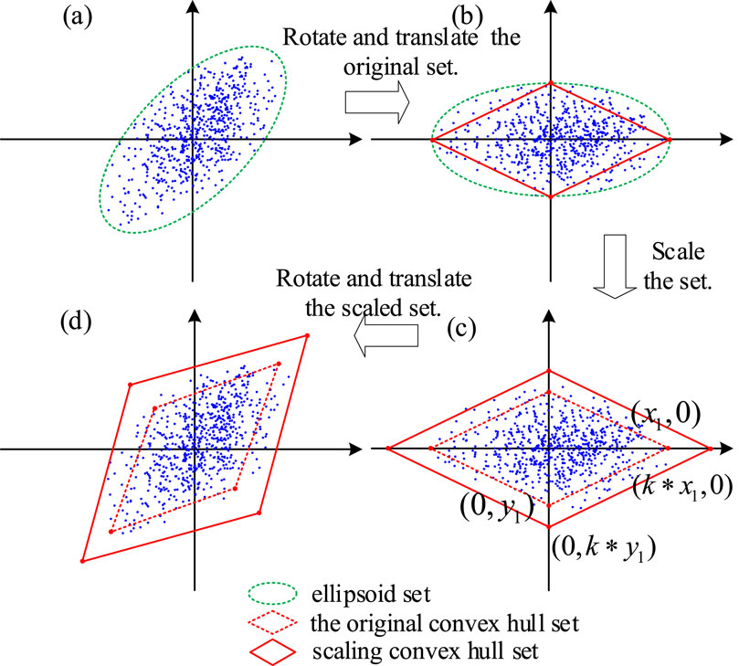
Figure 3. The modeling process for the convex hull uncertainty set (parts (a–d) illustrate key transformation steps).

Step (1): Firstly, construct a high-dimensional ellipsoidal uncertainty set that covers all historical data fluctuations with minimal volume, as illustrated in Figure 3a. The specific representation is given by Equation 5, which is:

${\mathit{U}}_{e1}=\left\{\mathit{z}\in {\mathit{R}}^{N\times 1}|{\left(\mathit{z}-\mathit{c}\right)}^{\mathrm{T}}{\mathit{\Sigma }}^{-1}\left(\mathit{z}-\mathit{c}\right)\le 1\right\}(5)$

Step (2): On the basis of the original high-dimensional ellipsoid, perform an orthogonal decomposition of the positive definite matrix $\mathit{\Sigma }$ into matrix $\mathit{\Sigma }={\mathit{P}}^{\mathit{T}}\mathit{J}\mathit{P}={\mathit{P}}^{-1}\mathit{J}\mathit{P}$. Rotate and translate the existing ellipsoid so that its center coincides with the origin of the coordinate axes, as shown by the green dashed line in Figure 3b. At this point, the high-dimensional ellipsoidal uncertainty set becomes ${\mathit{U}}_{e2}$, which is shown in Equation 6:

${\mathit{U}}_{e2}=\left\{{\mathit{z}}^{\prime }\in {\mathit{R}}^{N\times 1}|{\left({\mathit{z}}^{\prime }\right)}^{\mathrm{T}}{\mathit{J}}^{-1}\left({\mathit{z}}^{\prime }\right)\le 1\right\}(6)$

${\mathit{z}}^{\prime }=\mathit{P}\times \left(\mathit{z}-\mathit{c}\right)(7)$

where $\mathit{J}$ is a diagonal matrix, denoted as $\mathit{J}=\text{diag}\left({\lambda }_1\dots {\lambda }_N\right)$; P is a transformation matrix, representing the offset angle of the matrix.

Given the diagonal matrix $\mathit{J}$, the coordinates of the vertices ${z_{c,i}}^{\prime }$ of the transformed high-dimensional ellipsoid are shown in Equation 8:

$\left\{\begin{array}{l}{z_{c,1}}^{\prime }=\left[1/\sqrt{{\lambda }_1},0\dots 0\right],{z_{c,N+1}}^{\prime }=-\left[1/\sqrt{{\lambda }_1},0\dots 0\right]\\ {z_{c,2}}^{\prime }=\left[0,1/\sqrt{{\lambda }_2}\dots 0\right],{z_{c,N+2}}^{\prime }=-\left[0,1/\sqrt{{\lambda }_2}\dots 0\right]\\ ⋮\\ {z_{c,N}}^{\prime }=\left[0,0\dots 1/\sqrt{{\lambda }_{N_{\text{PV}}}}\right],{z_{c,2N}}^{\prime }=-\left[0,0\dots 1/\sqrt{{\lambda }_N}\right]\end{array}\right.(8)$

where $m_i$ represents the weight coefficient of the i-th vertex.

Step (3): Due to the high-dimensional linear polyhedral set obtained from step 2, a small number of data points fall outside the envelope. Therefore, a scaling process is necessary for the original set, as shown by the solid lines in Figure 3c. After scaling, the vertices of the high-dimensional linear polyhedron are shown in Equation 9:

$\left\{\begin{array}{l}k{z_{c,1}}^{\prime }=\left[k/\sqrt{{\lambda }_1},0\dots 0\right],k{z_{c,N+1}}^{\prime }=-\left[k/\sqrt{{\lambda }_1},0\dots 0\right]\\ k{z_{c,2}}^{\prime }=\left[0,k/\sqrt{{\lambda }_2}\dots 0\right],k{z_{c,N+2}}^{\prime }=-\left[0,k/\sqrt{{\lambda }_2}\dots 0\right]\\ ⋮\\ k{z_{c,N}}^{\prime }=\left[0,0\dots k/\sqrt{{\lambda }_N}\right],k{z_{c,2N}}^{\prime }=-\left[0,0\dots k/\sqrt{{\lambda }_N}\right]\end{array}\right.(9)$

At this point, the scaled high-dimensional linear polyhedral uncertainty set ${\mathit{U}}_{p2}$ is shown in Equation 10:

${\mathit{U}}_{p2}=\left\{{\mathit{z}}^{\prime }\in {\mathit{R}}^{N\times 1}\left|\begin{array}{l}{\mathit{z}}^{\prime }={\displaystyle \sum _{i=1}^{2N}}{m}_{i}k{{\mathit{z}}_{c,i}}^{\prime }\\ {\displaystyle \sum _{i=1}^{2N}}{m}_i=1;0\le m_i\le 1\end{array}\right.\right\}(10)$

where $k$ is the scaling factor, used to adjust the conservativeness of the high-dimensional linear polyhedral envelope range. The calculation method for $k$ is detailed in Moradian et al. (2024), thus there exists a minimum $k_{\min }$ that ensures the scaled polyhedral set precisely envelops all possible data points. The derivation process of $k_{\min }$ is shown in Supplementary Appendix SA1. Consequently, the valid range for $k$ is $\left[0,k_{\min }\right]$, and the polyhedral sets formed by different values of $k$ are illustrated in Figure 4.

Figure 4

Figure 4. The range of convex hull sets under different values of k.

The scaling factor influences the degree to which the convex hull set envelops data points. When $k=1$, the convex hull set, formed by connecting the ellipsoid’s endpoints, does indeed envelop all historical PV output points. However, it fails to fully account for certain extreme scenarios, which, while reducing the conservativeness of the optimization outcomes, compromises the system’s robustness. By gradually increasing the scaling factor of the convex hull set until it equals $k_{\min }$, the set now fully encompasses all historical output points. Unlike the box set, it minimally envelops blank areas, thus, while decreasing the conservativeness of the optimization results, it enhances the robustness of the outcomes simultaneously.

Step (4): Rotate and translate the scaled high-dimensional linear polyhedron so that it conforms to the original data points’ range. From Equation 7, it is known that after rotation and translation, the high-dimensional linear polyhedral uncertainty set ${\mathit{U}}_{p1}$ is shown in Equation 11:

${\mathit{U}}_{p1}=\left\{\mathit{z}\in {\mathit{R}}^{N\times 1}\left|\begin{array}{l}\mathit{z}={\displaystyle \sum _{i=1}^{2N}}{m}_i\left(\mathit{c}+k{\mathit{P}}^{-1}{{\mathit{z}}_{c,i}}^{\prime }\right)\\ {\displaystyle \sum _{i=1}^{2N}}{m}_i=1;0\le m_i\le 1\end{array}\right.\right\}(11)$

In summary, when the box set is used to describe the fluctuation of photovoltaic output, because it is an interval set, as shown in the black box square box line in Figure 4. Although it completely envelopes all the possibilities of photovoltaic output, due to the existence of a large number of blank areas, the results obtained by using this set are conservative to a certain extent. When the convex hull set is used, it is shown in the color diamond box in Figure 4. Since it is connected by the endpoints of the elliptical set and the polyhedron set obtained by scaling, it has a good ability to describe the historical output points of the photovoltaic, and reduces the envelope of the blank area while completely enveloping. This solves the disadvantage of high conservatism brought by the box set.

3 Industrial park microgrid optimization modeling

3.1 Industrial park microgrid system

The power-to-gas industrial park microgrid system is an integrated system that combines electricity, thermal energy, and gas energy, typically involving various energy conversion and utilization technologies, aiming to achieve efficient energy utilization and complementarity.

The typical power-to-gas industrial park microgrid system established in this paper consists of the following components, and the industrial park microgrid system diagram is shown in Figure 5.

Figure 5

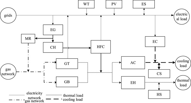
Figure 5. Industrial park microgrid system diagram.

Renewable energy facilities, including solar photovoltaic (PV) systems and wind turbine generation (WT) systems, which primarily convert renewable energy such as solar and wind power into electricity to supply electric loads; energy storage facilities, including battery energy storage systems (ES), heat storage systems (HS), and cold storage systems (CS), which not only provide energy to the system but also store excess energy for future use; heating equipment, such as gas boilers (GB) and excess heat boilers (EH); cooling equipment, such as absorption refrigerators (AC); and various energy conversion equipment, including gas turbines (GT), electroliers (EG), methane reactors (MR), hydrogen storage tanks (CH), hydrogen fuel cells (HFC), and electric chillers (EC).

3.2 Demand-side response model

In order to better accommodate clean energy and enhance the stability and economic efficiency of the system, a demand-side response model needs to be established on the load side. The model is constructed as follows:

$-{\xi }_t=\frac{\Delta P_t^{\mathrm{D}}}{\Delta {\rho }_t^{\mathrm{D}}}=\frac{P_t^{\mathrm{D},\text{cur}}-P_t^{\mathrm{D}}}{{\rho }_t^{\mathrm{D},\text{cur}}-{\rho }_t^{\mathrm{D}}}(12)$

${\displaystyle \sum _{t=1}^T}{P}_t^{\text{cur}}={\displaystyle \sum _{t=1}^T}{P}_t^{\mathrm{D}}(13)$

${\rho }_t^{\text{cur},\max }\le {\rho }_t^{\text{cur}}\le {\rho }_t^{\text{cur},\min }(14)$

${\rho }_t^{\text{cur}}=\left\{\begin{array}{l}{\rho }^{\text{peak}}t\in T^{\text{peak}}\\ {\rho }^{\text{valley}}t\in T^{\text{valley}}\end{array}\right.(15)$

where ${\xi }_t$ represents the price elasticity coefficient at the moment $t$; $\Delta P_t^{\mathrm{D}}$ represents the change in the demand-side load before and after the response is implemented at the moment $t$; $\Delta {\rho }_t$ represents the change in the demand-side electricity price before and after the response is implemented at the moment $t$; ${\rho }_t^{\mathrm{D}}$ and ${\rho }_t^{\mathrm{D},\text{cur}}$ respectively represent the electricity price before and after the demand side response is applied at the moment $t$; ${\rho }_t^{\text{cur},\max }$ and ${\rho }_t^{\text{cur},\min }$ respectively represent the upper and lower limits of the electricity price before and after the demand side response are applied at the moment $t$; ${\rho }^{\text{peak}}$ and ${\rho }^{\text{valley}}$ represent the peak and valley power before the demand-side response is implemented; $T^{\text{peak}}$ and $T^{\text{valley}}$ respectively represent the time periods of peak and valley power after the demand-side response is implemented. Equation 12 defines the elastic relationship between electricity price and load. Equation 13 ensures the balance of total electricity consumption before and after the response. Equation 14 defines the value range of electricity price. Equation 15 defines the peak and valley values of electricity price. The modeling of thermal load response follows the same logic.

3.3 IDR model

However, the demand-side response model only focuses on making response strategies for a single type of demand-side resource, in the power-to-gas industrial park microgrid system, due to the coordinated operation of multiple energy forms and equipment, the demand-side response model is difficult to coordinate the operation of multiple types of energy and equipment, an efficient adjustment model is needed to manage and optimize the operation of the system. Therefore, this paper adopts the Integrated Demand Response (IDR) model.

$0\le \Delta P_t^{0,\text{IDR}}\le P_t^{\text{IDR}}(16)$

$P_t^{\text{IDR}}\le P_{\max }^{\text{IDR}}(17)$

where $\Delta P_t^{0,\text{IDR}}$ represents the change of load when the system adopts the IDR model, $P_t^{\text{IDR}}$ represents the IDR reserve capacity of the load at the moment $t$, and $P_{\max }^{\text{IDR}}$ represents the maximum value of the IDR load. Equation 16 defines the range of load change, and Equation 17 specifies the conditions that the load reserve capacity must satisfy.

4 Objective function and constraints

4.1 Objective function

In this paper, we consider the electricity-gas multi-energy complementary microgrid model that minimizes the integrated cost of energy purchase cost, operation and maintenance cost, IDR cost, and standby cost, and is shown in Equation 18:

$\min \mathrm{C}={\mathrm{C}}_{\text{buy}}+{\mathrm{C}}_{\text{main}}+{\mathrm{C}}_{\text{SP}}+{\mathrm{C}}_{\text{IDR}}(18)$

Equations 19–22 respectively demonstrate the calculation methods for energy purchase cost, operation and maintenance cost, Integrated Demand Response (IDR) cost, and standby cost.

${\mathrm{C}}_{\text{buy}}={\displaystyle \sum _t^T}\left[\left(\frac{b_t^{\mathrm{e}}+s^e}{2}{P}_t^{\mathrm{E}}+\frac{b_t^{\mathrm{e}}-s^e}{2}\left|P_t^{\mathrm{E}}\right|\right)+b_t^{\mathrm{g}}{Q}_t^{\mathrm{G}}\right](19)$

where ${\mathrm{C}}_{\text{buy}}$ represents the cost of energy purchased by the system from the higher grid as well as from the gas grid; $P_t^{\mathrm{E}}$ represents the power of interaction between the system and the grid at time t. A positive value indicates that power is purchased from the grid, while a negative value indicates that power is sold to the grid; $Q_t^{\mathrm{G}}$ represents the natural gas purchased by the system at time t; $b_t^{\mathrm{e}}$ and $b_t^{\mathrm{g}}$ represent the price of the electricity and natural gas, respectively, at the time of purchase at time t; and $s^e$ represents the price of the electricity at the time of sale.

${\mathrm{C}}_{\text{main}}={\displaystyle \sum _n^N}{\displaystyle \sum _t^T}{c}^n{P}_t^n(20)$

where $c^n$ denotes the number of O&M coefficients of the nth device; $P_t^n$ denotes the output of the nth device at time t.

${\mathrm{C}}_{\text{SP}}={\displaystyle \sum _t^T}\left(c_{\text{sp}}^{+}{P}_t^{\text{sp},+}+c_{\text{sp}}^{-}{P}_t^{\text{sp},-}\right)(21)$

where $c_{\text{sp}}^{+}$ and $c_{\text{sp}}^{-}$ denote the upward and downward standby cost coefficients of the grid; $P_t^{\text{sp},+}$ and $P_t^{\text{sp},-}$ denote the upward and downward standby capacity of the grid at time t, respectively.

${\mathrm{C}}_{\text{IDR}}={\displaystyle \sum _t^T}\left(c_{\text{IDR}}{P}_t^{\text{IDR}}\right)(22)$

where ${\mathrm{C}}_{\text{IDR}}$ denotes the cost factor when the user participates in IDR.

4.2 Constraint condition

4.2.1 Energy balance constraints

The expression for the electrical power balance of the system is shown in Equation 23:

$\begin{array}{l}{P}_t^{\mathrm{E}}-P_t^{\text{EG}}+{\eta }^{\text{HFCE}}{P}_t^{\text{CH},\text{out}}+{\eta }^{\text{GTE}}{Q}_t^{\text{GT}}+P_t^{\text{WT}}\\ +P_t^{\text{PV}}+P_t^{\text{ES},\text{dis}}-P_t^{\text{ES},\text{ch}}-P_t^{\text{EC}}=P_t^{\mathrm{D},\text{cur}}-\Delta P_t^{0,\text{IDR}}\end{array}(23)$

where $P_t^{\text{EG}}$, $P_t^{\text{CH},\text{out}}$, $P_t^{\text{WT}}$, $P_t^{\text{PV}}$, $P_t^{\text{ES},\text{dis}}$, $P_t^{\text{ES},\text{ch}}$, $P_t^{\text{EC}}$ indicate the size of the electrolyzer, hydrogen storage tank, distributed wind power, distributed photovoltaic, battery storage, electric refrigeration machine at the moment t to consume or send out the size of the electric energy; $Q_t^{\text{GT}}$ indicates that the gas turbine at the moment t of the size of the gas-to-electricity power; ${\eta }^{\text{HFCE}}$ indicates that the electric efficiency of the hydrogen fuel cell; ${\eta }^{\text{GTE}}$ indicates that the gas turbine gas-to-electricity efficiency.

The gas balance expression for the system is shown in Equation 24:

$Q_t^{\mathrm{G}}+{\eta }^{\text{MR}}{Q}_t^{\text{MR}}-Q_t^{\text{GT}}-Q_t^{\text{GB}}=0(24)$

where $Q_t^{\text{MR}}$ represents the amount of natural gas injected into the system by the methane reactor at the moment t; $Q_t^{\text{GB}}$ represents the amount of natural gas consumed by the gas boiler at the moment t; and ${\eta }^{\text{MR}}$ represents the natural gas generation efficiency of the methane generator.

The heat balance expression of the system is shown in Equation 25:

${\eta }^{\text{EH}}{P}_t^{\text{EH}}+P_t^{\text{HS},\text{dis}}-P_t^{\text{HS},\text{ch}}=P_t^{\mathrm{H}}(25)$

where $P_t^{\text{EH}}$ represents the thermal power produced by the waste heat boiler at the moment t; $P_t^{\text{HS},\text{dis}}$ and $P_t^{\text{HS},\text{ch}}$ represent the thermal power issued or stored in the heat storage tank at the moment t respectively; $P_t^{\mathrm{H}}$ represents the thermal load of the system at the moment t; ${\eta }^{\text{EH}}$ represents the heat production efficiency of the waste heat boiler.

The cold balance expression of the system is shown in Equation 26:

${\eta }^{\text{AC}}{P}_t^{\text{AC}}+{\eta }^{\text{EC}}{P}_t^{\text{EC}}+P_t^{\text{CS},\text{dis}}-P_t^{\text{CS},\text{ch}}=P_t^{\mathrm{C}}(26)$

where $P_t^{\text{AC}}$ represents the cold energy power issued by the absorption chiller at the moment t; $P_t^{\text{CS},\text{dis}}$ and $P_t^{\text{CS},\text{ch}}$ represent the cold energy power issued or stored in the cold storage tank at the moment t, respectively; $P_t^{\mathrm{C}}$ represents the cold load of the system at the moment t; ${\eta }^{\text{AC}}$ and ${\eta }^{\text{EC}}$ represent the refrigeration efficiency of the absorption chiller, respectively.

4.2.2 Energy coupling constraints

Electricity - gas conversion mainly includes two aspects of electricity hydrogen and hydrogen methanization, the system of electricity - gas conversion coupling constraints expression is shown in Equation 27:

${\eta }^{\text{EG}}{P}_t^{\text{EG}}-Q_t^{\text{MR}}-P_t^{\text{CH},\text{in}}=0(27)$

where ${\eta }^{\text{EG}}$ represents the efficiency of the electrolyzer to convert gas; $P_t^{\text{CH},\text{in}}$ represents the amount of hydrogen input to the hydrogen storage tank at the moment t. The system heat-cooling conversion is mainly to convert part of the system heat power into cold power.

The heat-cooling conversion is mainly to convert part of the input thermal power of the system into cold power, and the expression of the coupling constraints of heat-cooling conversion of the system is as follows

${\eta }^{\text{HFCH}}{P}_t^{\text{CH},\text{out}}+{\eta }^{\text{GB}}{Q}_t^{\text{GB}}+{\eta }^{\text{GT}}{Q}_t^{\text{GT}}=P_t^{\text{AC}}+P_t^{\text{EH}}(28)$

where ${\eta }^{\text{HFCH}}$ represents the thermal efficiency of the hydrogen fuel cell, ${\eta }^{\text{GB}}$ and ${\eta }^{\text{GT}}$ represent the thermal efficiency of the gas boiler and gas turbine respectively.

4.2.3 Operation constraints of energy supply equipment

The operation constraints of each device in the system are expressed as Equations 29, 30

$P_{\min }^n\le P_t^n\le P_{\max }^n(29)$

$\Delta P_{\min }^n\le P_{t+1}^n-P_t^n\le \Delta P_{\max }^n(30)$

where $P_{\min }^n$ and $P_{\max }^n$ represent the upper and lower limits of the n-th equipment output, $\Delta P_{\min }^n$ and $\Delta P_{\max }^n$ represent the upper and lower limits of the nth equipment output change in the neighboring time period.

4.2.4 Energy storage operation constraints

$S_t^m=S_{t-1}^m+{\eta }^{m,\text{ch}}{P}_t^{m,\text{ch}}-\frac{P_t^{m,\text{dis}}}{{\eta }^{m,\text{dis}}}(31)$

$\left\{\begin{array}{l}0\le P_t^{m,\text{ch}}\le P_{\max }^{m,\text{ch}}{D}_t^{m,\text{ch}}\\ 0\le P_t^{m,\text{dis}}\le P_{\max }^{m,\text{dis}}{D}_t^{m,\text{dis}}\\ D_t^{m,\text{ch}}+D_t^{m,\text{dis}}\le 1\end{array}\right.(32)$

$S_{\min }^m\le S_t^m\le S_{\max }^m(33)$

$S_T^m=S_1^m(34)$

where $S_t^m$ denotes the size of energy stored in the m-th storage device at the moment t, $P_t^{m,\text{ch}}$ and $P_{\max }^{m,\text{ch}}$ denote the maximum charging and discharging power of the m-th storage device at the moment t, ${\eta }^{m,\text{ch}}$ and ${\eta }^{m,\text{dis}}$ denote the charging and discharging efficiency of the m-th storage device, $D_t^{m,\text{ch}}$ and $D_t^{m,\text{dis}}$ denote the charging and discharging state of the m-th storage device at the moment t, respectively. Equations 31–34 sequentially define the dynamic change relationship of the stored energy of energy storage devices, the constraints on charging/discharging power and status, the limitation on the range of stored energy, and the closed - loop condition for the stored energy at the start and end of the period, regulating the operation process of the energy storage system.

4.2.5 Hydrogen storage tank operation constraints

Similar to the battery energy storage, the hydrogen storage tank can also be regarded as an energy storage device.

$S_t^{\text{CH}}=S_{t-1}^{\text{CH}}+{\eta }^{\text{CH},\text{in}}{P}_t^{\text{CH},\text{in}}-\frac{P_t^{\text{CH},\text{out}}}{{\eta }^{\text{CH},\text{out}}}(35)$

$\left\{\begin{array}{l}0\le P_t^{\text{CH},\text{in}}\le P_{\max }^{\text{CH},\text{in}}{D}_t^{\text{CH},\text{in}}\\ 0\le P_t^{\text{CH},\text{out}}\le P_{\max }^{\text{CH},\text{out}}{D}_t^{\text{CH},\text{out}}\\ D_t^{\text{CH},\text{in}}+D_t^{\text{CH},\text{out}}\le 1\end{array}\right.(36)$

$S_{\min }^{\text{CH}}\le S_t^{\text{CH}}\le S_{\max }^{\text{CH}}(37)$

$S_T^{\text{CH}}=S_1^{\text{CH}}(38)$

where $S_t^{\text{CH}}$ represents the amount of hydrogen stored in the hydrogen storage tank at the moment t, $P_t^{\text{CH},\text{in}}$ and $P_t^{\text{CH},\text{out}}$ represent the maximum hydrogen filling and discharging capacities of the hydrogen storage tank at the moment t, ${\eta }^{\text{CH},\text{in}}$ and ${\eta }^{\text{CH},\text{out}}$ represent the hydrogen filling and discharging efficiency of the hydrogen storage tank, $D_t^{\text{CH},\text{in}}$ and $D_t^{\text{CH},\text{out}}$ represent the hydrogen filling and discharging energy state of the hydrogen storage tank at the moment t. Equations 35–38 sequentially define the dynamic change of hydrogen storage amount in hydrogen storage tanks, the constraints on hydrogen charging/discharging power and status, the range of hydrogen storage amount, and the periodic closed-loop condition.

4.2.6 Power exchange constraints in large power grids

$P_t^{\mathrm{E}}+P_t^{\text{sp},+}\le P_{\max }^{\mathrm{E}}(39)$

$P_t^{\mathrm{E}}-P_t^{\text{sp},+}\ge P_{\min }^{\mathrm{E}}(40)$

where $P_{\max }^{\mathrm{E}}$ and $P_{\min }^{\mathrm{E}}$ respectively represent the upper and lower limits of power exchange with the large power grid. Equation 39 defines the upper limit of the power exchange combined with the upward reserve, and Equation 40 specifies the lower limit of the power exchange after deducting the upward reserve.

4.2.7 Constraint on reserve capacity

In order to ensure the reasonable reserve capacity of the system, the constraints are set as Equations 41–43.

$0\le P_t^{\text{sp},+}\le P_{\max }^{\text{sp},+}(41)$

$P_{\min }^{\text{sp},-}\le P_t^{\text{sp},-}\le P_{\max }^{\text{sp},-}(42)$

$P_t^{\text{sp},+}+P_t^{\text{IDR}}\ge P_{\min }^{\text{sp},+}(43)$

where $P_{\max }^{\text{sp},+}$ and $P_{\max }^{\text{sp},-}$ respectively represent the maximum values of upward and downward reserves, and $P_{\min }^{\text{sp},-}$ represents the minimum value of downward reserves.

4.2.8 Constraint on output of renewable energy

The constraints of renewable energy are as Equations 44, 45.

$0\le P_t^{\text{WT}}\le {\stackrel{\sim }{P}}_t^{\text{WT}}(44)$

$0\le P_t^{\text{PV}}\le {\stackrel{\sim }{P}}_t^{\text{PV}}(45)$

5 Robust optimization method for microgrid in industrial park

5.1 Robust optimization model establishment

Let the renewable energy constraint variable of the system be vector ${\mathit{P}}^{\text{RE}}=\left\{P_t^{\text{PV}},P_t^{\text{WT}}\right\}$; the constraint variable of energy storage equipment be vector ${\mathit{P}}^{\text{ES}}=\left\{S_t^m,P_t^{m,\text{ch}},P_t^{m,\text{dis}}\right\}$; the constraint variable of energy supply equipment be vector ${\mathit{P}}^{\mathrm{E}}=\left\{P_t^n\right\}$; the operation constraint variable of hydrogen storage tank be vector ${\mathit{P}}^{\text{CH}}=\left\{S_t^{\text{CH}},P_t^{\text{CH},\text{in}},P_t^{\text{CH},\text{out}}\right\}$; the energy purchase constraint variable be vector ${\mathit{P}}^{\text{SP}}=\left\{P_t^{\mathrm{E}},Q_t^{\mathrm{G}},P_t^{\text{sp},+},P_t^{\text{sp},-}\right\}$; and the IDR constraint variable be vector ${\mathit{P}}^{\text{IDR}}=\left\{\Delta P_t^{0,\text{IDR}},P_t^{\text{IDR}}\right\}$. Then, the matrix form of the robust optimization model for the microgrid in the industrial park established in this paper is as Equation 46.

$\begin{array}{cc}\hfill & \hfill \underset{x}{\min }\left(\underset{u\in \mathit{U}}{\max }\underset{\mathit{y}\in \mathrm{\Omega }\left(\mathit{x},\mathit{u}\right)}{\min }{\mathit{c}}^{\mathrm{T}}\mathit{y}\right)\\ s.t.\hfill & \hfill \mathit{A}\mathit{x}\le \mathit{d}\left(\mathrm{a}\right)\\ \hfill & \hfill \mathit{G}\mathit{y}\le \mathit{h}-\mathit{E}\mathit{x}-\mathit{M}\mathit{u}\left(\mathrm{b}\right)\end{array}(46)$

where $\mathit{x}$ and $\mathit{y}$ are the decision variables of the model, and $\mathit{u}$ is the uncertain variable. Among them, the first-stage decision variables $\mathit{x}=\left\{D_t^{m,\text{ch}},D_t^{m,\text{dis}}\right\}$, $D_t^{m,\text{ch}}$, and $D_t^{m,\text{dis}}$ represent the charging and discharging states of the m-th energy storage system; the second-stage decision variable is $\mathit{y}=\left\{{\mathit{P}}^{\text{RE}},{\mathit{P}}^{\text{ES}},{\mathit{P}}^{\mathrm{E}},{\mathit{P}}^{\text{CH}},{\mathit{P}}^{\text{SP}},{\mathit{P}}^{\text{IDR}}\right\}$; the second-stage uncertain variable is $\mathit{u}=\left\{{\stackrel{\sim }{P}}_t^{\text{PV}},{\stackrel{\sim }{P}}_t^{\text{WT}}\right\}$. The constant matrix $\mathit{A}$ represents the coefficient matrix related to the decision variable $\mathit{x}$. The column vector $\mathit{d}$ is a constant and represents the coefficient vector related to the decision variable $\mathit{x}$. The constant matrices $\mathit{G}$ and $\mathit{E}$ represent the coefficient matrices related to the decision variable $\mathit{y}$. The column vector $\mathit{h}$ is a constant vector and represents the coefficient vector related to the decision variable $\mathit{y}$. The constant matrix $\mathit{M}$ represents the coefficient matrix related to the uncertain variable $\mathit{u}$. $\mathrm{\Omega }\left(\mathit{x},\mathit{u}\right)$ is the feasible region of the continuous variable $\left(\mathit{x},\mathit{u}\right)$ when $\mathit{y}$ is given. ${\mathit{c}}^{\mathrm{T}}\mathit{y}$ represents the objective function of the second stage, corresponding to Equations 19 and 47 corresponds to the constraint condition related to the first-stage variable $\mathit{x}$; (47-b) corresponds to the constraint condition related to the second-stage variable $\mathit{y}$.

For a two-stage robust optimization model like Equation 47, since it contains both continuous variables and integer variables, and the second stage of the model contains uncertain parameter $\mathit{u}$, it cannot be directly solved. Therefore, this paper uses method $\mathrm{C}\&\text{CG}$ (Nayak et al., 2025; Michos et al., 2024) to transform it into a master-slave problem for solution. Among them, the master problem is to solve the integrated energy optimization model with the minimum comprehensive cost under the worst case; the sub-problem is to first solve the integer solution of the master problem (such as the charging and discharging state of the energy storage battery), and then optimize the remaining continuous variables to minimize the comprehensive cost obtained by the system under the worst case.

5.2 C&CG iterative solution method

The master-slave problem corresponding to Equation 47 is modeled as

$\text{MP}1:\left\{\begin{array}{l}\underset{x,y,u}{\min }\left(\eta \right)\\ s.t.\mathit{A}\mathit{x}\le \mathit{d}\\ \mathit{G}{\mathit{y}}^l\le \mathit{h}-\mathit{E}\mathit{x}-\mathit{M}{\mathit{u}}^l\forall l\le k\\ \eta \ge {\mathit{c}}^{\mathrm{T}}{\mathit{y}}^l\forall l\le k\end{array}\right.(47)$

$\text{SP}1:\left\{\begin{array}{l}\underset{u\in \mathit{U}}{\max }\underset{y\in \mathrm{\Omega }\left(x,u\right)}{\min }{\mathit{c}}^{\mathrm{T}}\mathit{y}\\ s.t.\mathit{G}\mathit{y}\le \mathit{h}-\mathit{E}{\mathit{x}}^{*}-\mathit{M}\mathit{u}:\mathit{\pi }\end{array}\right.(48)$

The main problem MP1 corresponding to Equation 48 is solved first, at this point, MP1 belongs to the mixed-integer second-order cone programming problem. After solving the first-stage variable solution $\mathit{x}*$ corresponding to MP1 and the auxiliary variable $\eta$ introduced in $k+1$ iterations, which is $\mathrm{C}\&\text{CG}$-cut. Then, the variable solution $\mathit{x}*$ derived in the first stage is brought into the second stage subproblem SP1 to find the worst-case scenario ${\mathit{u}}^l$ , where l is the number of historical iterations and k is the number of current iterations. Finally, the worst-case scenario ${\mathit{u}}^l$ solved in the second stage is brought into the main problem MP1 of the first stage and iterated. Where the last three constraints of Equation 48 are the set of optimal and feasible cut planes resulting from the previous k iterations, respectively. $\mathit{\pi }$ is the dyadic variable of the subproblem constraints.

5.2.1 Sub-problem solution method

Equation 49 is a max-min optimization problem, therefore, in this paper, the pairwise theorem is used to convert the inner min problem of Equation 49 into its pairwise form to merge it into a maximization problem, which is shown in the form of Equation 50.

$\begin{array}{cc}\hfill & \hfill \underset{u,\pi }{\max }-{\left(\mathit{h}-\mathit{M}\mathit{u}-\mathit{E}\mathit{x}\right)}^{\mathrm{T}}\mathit{\pi }\\ s.t.\hfill & \hfill \mathit{c}+{\mathit{N}}^{\mathrm{T}}\mathit{\pi }=0\\ \hfill & \hfill \mathit{\pi },{\mathit{\tau }}^a,{\mathit{\tau }}^b\ge 0\end{array}(49)$

in Equation 50, there exists a bilinear term ${\left(\mathit{M}\mathit{u}\right)}^{\mathrm{T}}\mathit{\pi }$ , which is solved here by using the outer approximation of the bilinear term. The master problem MP2 and subproblem SP2 are obtained as shown in Equations 51 and 52.

$\text{SP}2:\left\{\begin{array}{l}\underset{u,\pi }{\max }-{\left(\mathit{h}-\mathit{M}\mathit{u}-\mathit{E}\mathit{x}\right)}^{\mathrm{T}}\mathit{\pi }\\ s.t.\mathit{c}+{\mathit{N}}^{\mathrm{T}}\mathit{\pi }=0\\ \mathit{\pi },{\mathit{\tau }}^a,{\mathit{\tau }}^b\ge 0\end{array}\right.(50)$

$\text{MP}2:\left\{\begin{array}{l}\underset{u,\pi }{\max }-{\left(\mathit{h}-\mathit{E}\mathit{x}\right)}^{\mathrm{T}}\mathit{\pi }+\mathit{\beta }\\ s.t.\mathit{c}+{\mathit{N}}^{\mathrm{T}}\mathit{\pi }=0\\ \mathit{\pi },{\mathit{\tau }}^a,{\mathit{\tau }}^b\ge 0\\ \mathit{\beta }\le G^m\left(\mathit{u},\mathit{\pi }\right),\forall m\le n\end{array}\right.(51)$

where MP2 and SP2 are used to solve the upper and lower bounds of Equation 38, respectively, $m$ is the number of historical iterations, and $n$ is the number of current iterations. An auxiliary variable $\mathit{\beta }$ is introduced to replace the bilinear term in the original equation, and a bilinear term exists in Equation 52 $G^m\left(\mathit{u},\mathit{\pi }\right)={\left(\mathit{M}\mathit{u}\right)}^{\mathrm{T}}\mathit{\pi }$. Therefore, it is necessary to use the outer approximation method for linearization, and the linearization formula is shown in (53).

$G^n\left(\mathit{u},\mathit{\pi }\right)={\left({\mathit{u}}^n\right)}^{\mathrm{T}}{\mathit{\pi }}_{sp}^n+{\left(\mathit{u}-{\mathit{u}}^n\right)}^{\mathrm{T}}{\mathit{\pi }}_{sp}^n+{\left(\mathit{\pi }-{\mathit{\pi }}_{sp}^n\right)}^{\mathrm{T}}{\mathit{u}}^n(52)$

6 Example analysis

This section is validated using the IEEE-RTS 24 node example system. To reflect the planning requirements of the power generation and transmission system, the load will be increased by 1.4 times. At the same time, 400 MW wind farms were connected at nodes 3, 6, 15, 18, and 23, respectively. According to Equation 28, the predicted wind power output value is about 115 MW, and the fluctuation of wind power output is ±30% of the predicted value. The typical value of sub transient reactance for all units is 0.1 (standard value). This example has two voltage levels, namely, 138 kV and 230 kV, and the maximum allowable current of the circuit breaker is 31.5 kA and 35 kA, respectively. The abandonment cost and load shedding cost are $150/(MWh) and $5,000/(MWh) respectively. This article considers N-1 random faults in power generation and transmission, and the convergence threshold of the C&CG algorithm ζ Set to 0.001.

6.1 Example setting

In order to verify the effectiveness of the data-driven industrial park microgrids robust optimization method established in this paper, this section cites a 24-h operation example of an industrial park in Hubei Province for verification. The equipment installed in the industrial park includes wind power, photovoltaic, gas boiler and waste heat boiler. Absorption chillers, gas turbines, electroliers, methane reactors, hydrogen storage tanks, hydrogen fuel cells, electric chillers, energy storage systems, etc. Among them, the wind power, photovoltaic prediction and load size of the system are shown in Figure 6. The operating parameters of each device are shown in. The operating parameters of each device are shown in Schedule A1. According to the calculation method given in (Hamed and Rasoul, 2021), the value $k_{\min }$ here is 1.22.

Figure 6

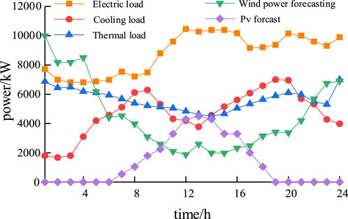
Figure 6. Renewable energy forecast output and load size.

Table 1

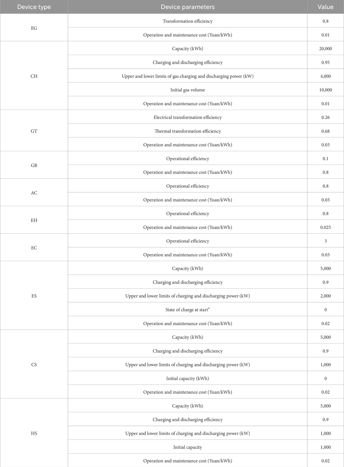
Table 1. Operation parameters of each device.

6.2 Result analysis and verification

6.2.1 The influence of scaling factor k on the optimization results

The impact of the scaling factor on the robust optimization of the industrial park microgrid is shown in Table 2. The size of the scaling factor determines the extent to which the constructed convex hull set covers historical data. As seen from Table 2, with the increase of the scaling factor, the system’s operational cost gradually decreases, while the energy purchase cost continues to increase. This is because the increase in the scaling factor expands the envelope range of the convex hull uncertainty set over the historical output data, meaning that the fluctuation range of renewable energy output becomes larger, making the worst-case scenario more likely to occur. When volatile renewable energies such as distributed photovoltaics and wind power continuously inject into the distribution network, in order to maintain supply-demand balance and reduce disturbances caused by the injection of uncertain energy, the system needs to filter out a large portion of the power injected by distributed photovoltaics and wind power. This leads to a reduction in the maintenance cost of photovoltaic and wind power equipment, and as a result, the overall operational cost decreases. Meanwhile, since the injection of distributed energy is reduced, more injection power from the grid is needed to meet the system’s electricity supply, thereby gradually increasing the energy purchase cost. Reserve cost refers to the margin cost incurred to account for the system’s response to possible random events and depends on the system’s contingency plan for the worst-case scenario. Therefore, regardless of changes in the scaling factor, the reserve cost shows little variation. Similar to the reserve cost, the IDR (Interruptible Demand Response) cost is an added cost to enhance the system’s stability margin. When the scaling factor is less than or equal to 1, the convex hull set does not envelop the extreme worst-case conditions, and thus the IDR cost remains unchanged. However, when the scaling factor exceeds 1, the convex hull set covers all possible scenarios, including the worst-case scenario. To improve the overall efficiency of the system, users need to appropriately shed load, which results in an increase in IDR cost.

Table 2

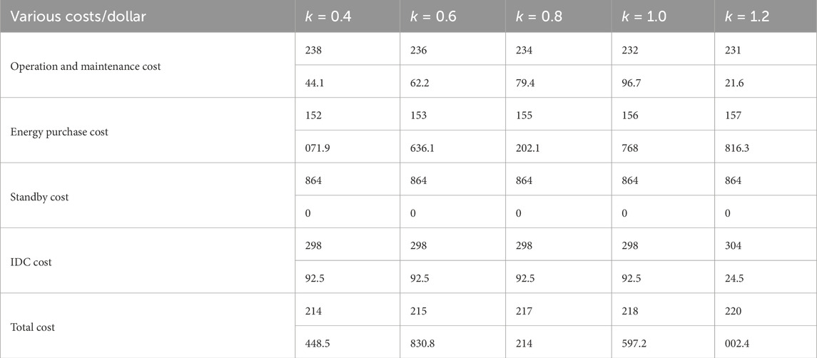
Table 2. The effect of scaling factor k on various costs.

6.2.2 The influence of robust adjustment coefficient β on the optimization results

Figure 7 demonstrates the influence of the robust adjustment coefficient β on the results of the robust optimization of the industrial park microgrid. From the figure, it can be seen that as the robust adjustment coefficient increases, each of the costs changes more or less, except for the standby cost, which is unaffected by system changes, which stays constant at $8640. When the robust adjustment coefficient of the system is small, the uncertain energy injected into the system at this time will be approximated as deterministic energy, the various equipment of the system will operate stably, and the photovoltaic and wind power equipment of the system will operate at full efficiency, so the operation and maintenance cost is the largest, and at the same time, due to the injection of the deterministic energy, the system purchased energy from the port decreases, so the system’s purchased energy cost is the smallest, and with the increase in the robust adjustment coefficient, this uncertainty energy injection will rise and the amount of energy purchased by the system from the port will keep on rising, which in turn leads to the rise of the system’s energy purchase cost and the decrease of the O&M cost. For the IDR cost, when $\beta \le 0.7$, the envelope always fails to cover the extreme conditions for both the boxed set and the convex packet set with different deflation multiples, so the IDR cost always stays the same; while when β is large, at this time, when the deflation multiples $k=k_{\min }$, the convex packet set will completely envelope the worst case when the deflation multiples are large, which will increase the IDR cost at this time, but due to the fact that the boxed set can not accurately envelope the distribution of the uncertain parameters, resulting in the blank area of the envelope. Region, resulting in more blank regions in the envelope, so the boxed set corresponds to the largest IDR cost compared to the convex packet set.

Figure 7

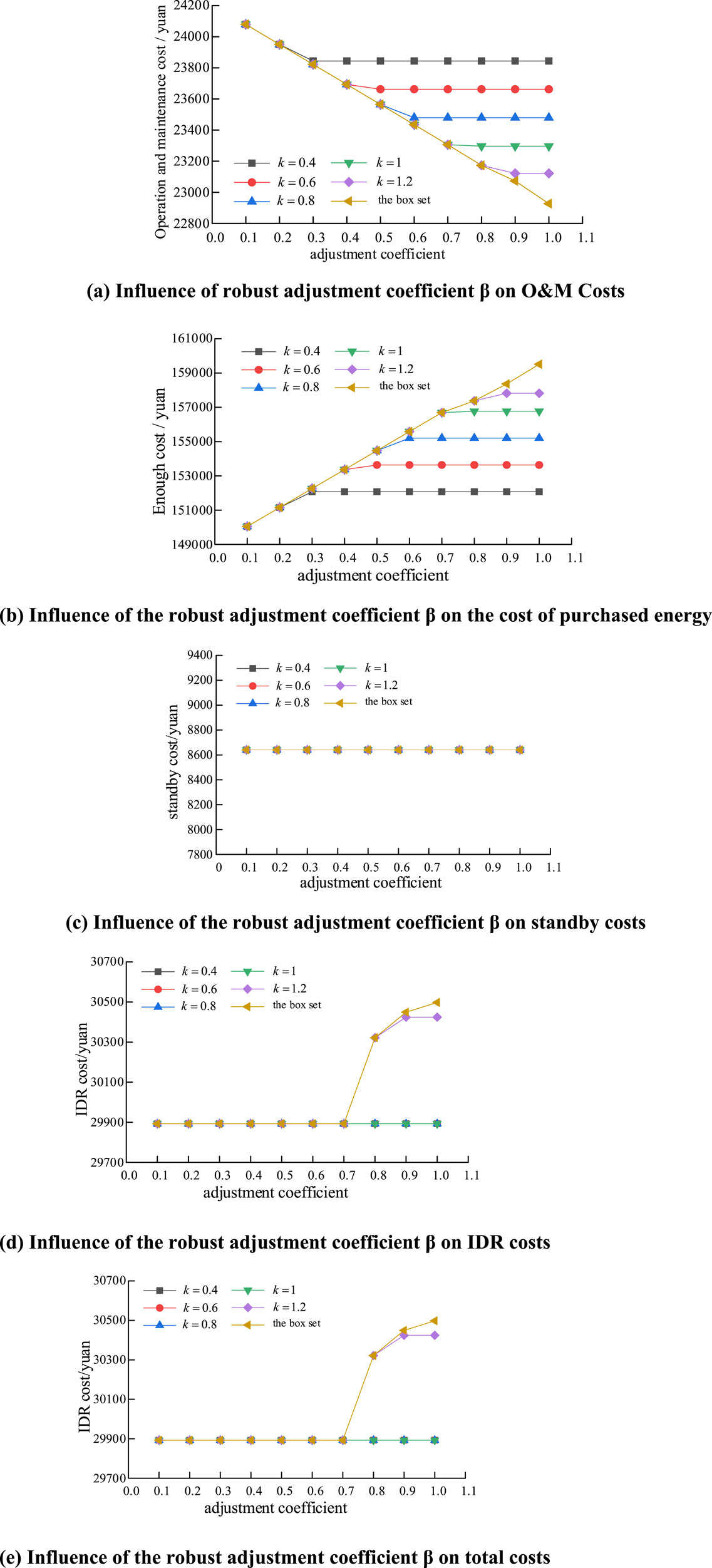
Figure 7. Influence of robust adjustment coefficient β on each cost. (a) Influence of robust adjustment coefficient β on O&M costs. (b) Influence of the robust adjustment coefficient β on the cost of purchased energy. (c) Influence of the robust adjustment coefficient β on standby costs. (d) Influence of the robust adjustment coefficient β on IDR costs. (e) Influence of the robust adjustment coefficient β on total costs.

As the robust adjustment coefficient increases, the magnitude of the change in the cost of purchased energy and O&M cost will remain stable when the convex packet ensemble is used, specifically, when the deflation multiplier increases from 0.4 to 1.2, the magnitude of the change in the cost of purchased energy and O&M cost will be stabilized at the time when the robust adjustment coefficient is equal to 0.3, 0.4, 0.6, 0.7, and 0.8, which is related to the renewable energy equipment’s power output situation. When β is small, the system is poorly adapted to the renewable energy perturbation and the cost does not change much no matter what kind of ensemble is used, on the contrary, when β is large, the system is better adapted to the distributed PV perturbation. However, when the convex packet ensemble is used, the envelope range of the convex packet ensemble is different due to different deflation multiples. When the deflation multiplier $k=0.4$, the envelope range of the convex packet ensemble is also smaller. In this case, changing the size of the robust regulation coefficient β will not significantly affect the renewable energy output size, so the effect of changing β to a certain extent on the renewable energy output will be minimal. However, when the deflation facto $k=k_{\min }$, the convex packet uncertainty set will encompass all the historical data, so it will be adjusted accordingly to the increase of the robust regulation coefficient β, which will affect the size of the renewable energy output. Since the purchased energy cost of the system accounts for a large proportion of the total cost, the trend of the total cost of the system is similar to that of the purchased energy cost.

6.2.3 The influence of the three aggregations on individual costs

The effects of the three uncertainty sets on each cost are further compared when the deflation multiplier $k=k_{\min }$, the robust adjustment coefficient $\beta =1$, and the uncertainty $\mathrm{\Gamma }=0.9$ are used, as shown in Table 3. From Table 3, it can be seen that when different sets are used, the total cost of using the convex packet set is lower than that of the box set and the polyhedral set, except that the standby cost remains basically the same. This is due to the fact that when there is spatio-temporal correlation of the uncertain parameters, the convex packet ensemble can change the envelope range of the convex packet ensemble by deflation to make it fit the distribution region of the uncertain parameters better, which enhances the robustness of the system and reduces the conservatism. On the other hand, the polyhedral set changes the envelope of the polyhedral set by changing the uncertainty, and in order to encompass the historical data of all renewable energy outputs, the polyhedral set needs to increase the uncertainty, which enables the expansion of the envelope of the polyhedral set in an untargeted manner, although this enhances the robustness of the solution results, but over-expansion for the sake of a few scenarios of the data increases the conservatism of the solution instead. The boxed ensemble, on the other hand, is a preliminary characterization of the uncertain parameter distribution range, and therefore the conservativeness and robustness of the solution results are the worst.

Table 3

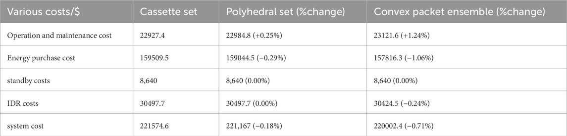
Table 3. The influence of the three aggregations on individual costs.

6.2.4 Output of each device in three pools

Figure 8 gives the output of each device at the electric power balance under the three uncertainty sets. From the figure, it can be seen that in the multi-energy complementary microgrid system, the individual devices coordinate with each other and work together to maintain the electric power balance. In the PV big hairy time period (12–16 h), the system purchases the lowest electric power from the ports, the polyhedral ensemble is the second, and the box ensemble is the most when the convex packet ensemble is used, which is the same as the conclusion obtained in the previous paper, and further verifies that the use of the convex packet ensemble enhances the robustness of the solution results and reduces the conservatism.

Figure 8

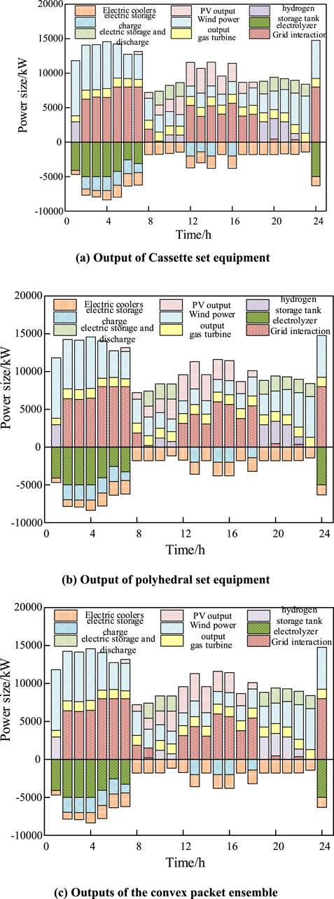
Figure 8. Output of each device under three aggregations. (a) Output of Cassette set equipment. (b) Output of polyhedral set equipment. (c) Outputs of the convex packet ensemble.

6.2.5 Computational efficiency analysis

To verify the computational efficiency of the convex hull uncertainty set, we supplemented simulation analyses comparing the convex hull set method with scenario-based stochastic optimization in the revised manuscript. The comparative results are shown in the table below.

As shown in Table 4, when handling problems of the same scale, the convex hull set method proposed in this paper exhibits significant computational efficiency advantages over scenario-based stochastic optimization. Even as the problem scale increases, the convex hull set method still outperforms scenario-based stochastic optimization in computational efficiency.

Table 4

Table 4. Comparative analysis of optimization methods.

7 Conclusion

In this paper, a research model of the industrial park microgrids robust optimization method based on data-driven is constructed and solved by C&CG algorithm. Finally, by comparing the industrial park microgrids robust optimization methods under different sets, the simulation results show that:

1. Compared with the interval set which can only take extreme conditions at the boundary, the polyhedron set has a better envelope for the range of uncertain parameters, which makes the operation result more robust.

2. When the robust adjustment coefficient is the same, the total system cost of using the convex hull set is 0.71% lower than that of the box set and 0.53% lower than that of the polyhedron set. For the convex hull set with different scaling multiples, this not only increases the envelope of the region with higher distribution of uncertain parameters, but also reduces the envelope of the blank region with low probability. Therefore, compared with the polyhedral set, the industrial park microgrids robust optimization method using the convex hull set is less conservative and more robust.

In the future, we will explore the comparative analysis between convex hull sets and advanced data-driven methods such as distributionally robust optimization and machine learning-based uncertainty sets, with a view to providing more comprehensive and forward-looking research results for the field of multi-energy microgrid optimization.

Data availability statement

The original contributions presented in the study are included in the article/Supplementary Material, further inquiries can be directed to the corresponding author.

Author contributions

CR: Investigation, Methodology, Writing – original draft. LL: Investigation, Methodology, Writing – original draft. JL: Validation, Writing – review and editing. BJ: Validation, Writing – review and editing.

Funding

The author(s) declare that financial support was received for the research and/or publication of this article. This work is supported by Science and Technology Project of State Grid Zhejiang Electric Power Co., Ltd. (No. 5211TZ230002).

Conflict of interest

Authors CR, JL, and BJ were employed by State Grid TaiZhou Power Supply Company.

Author LL was employed by State Grid ZheJiang Electric Power Corporation.

The authors declare that this study received funding from State Grid Zhejiang Electric Power Co. The funder participated in the research design phase. During this phase, combining the actual operation requirements of industrial park microgrids, it put forward relevant suggestions on the research direction (e.g., the industrial load characteristics that need to be focused on in microgrid robust optimization) and the practicality of the technical framework.

Generative AI statement

The author(s) declare that no Generative AI was used in the creation of this manuscript.

Any alternative text (alt text) provided alongside figures in this article has been generated by Frontiers with the support of artificial intelligence and reasonable efforts have been made to ensure accuracy, including review by the authors wherever possible. If you identify any issues, please contact us.

Publisher’s note

All claims expressed in this article are solely those of the authors and do not necessarily represent those of their affiliated organizations, or those of the publisher, the editors and the reviewers. Any product that may be evaluated in this article, or claim that may be made by its manufacturer, is not guaranteed or endorsed by the publisher.

Supplementary Material

The Supplementary Material for this article can be found online at: https://www.frontiersin.org/articles/10.3389/fenrg.2025.1535211/full#supplementary-material

References

Akter, K., Rahman, M., Islam, R. M., Sheikh, M. R. I., and Hossain, M. (2025). Attack-resilient framework for wind power forecasting against civil and adversarial attacks. Electr. Power Syst. Res. 238, 238111065–111065. doi:10.1016/j.epsr.2024.111065

CrossRef Full Text | Google Scholar

Aliasghar, B., Baseem, K., and Navid, P. (2022). Guest editorial: introduction to the special section on application of advanced machine/deep learning in electrical power and energy systems (VSI-mlep). Comput. Electr. Eng., 102. doi:10.1016/j.compeleceng.2022.108245

CrossRef Full Text | Google Scholar

Arooj, Q. (2024). FedWindT: Federated learning assisted transformer architecture for collaborative and secure wind power forecasting in diverse conditions. Energy 309, 133072–133072. doi:10.1016/j.energy.2024.133072

CrossRef Full Text | Google Scholar

Ayene, M. S., and Yibre, M. A. (2024). Wind power prediction based on deep learning models: the case of adama wind farm. Heliyon 10 (21), e39579. doi:10.1016/j.heliyon.2024.e39579

PubMed Abstract | CrossRef Full Text | Google Scholar

Bifei, T., Haoyong, C., and Xiaodong, Z. (2022). Two-stage robust optimization dispatch for multiple microgrids with electric vehicle loads based on a novel data-driven uncertainty set. Int. J. Electr. Power Energy Syst., 134. doi:10.1016/j.ijepes.2021.107359

CrossRef Full Text | Google Scholar

Davidsdottir, B., Ásgeirsson, I. E., Fazeli, R., Gunnarsdottir, I., Leaver, J., Shafiei, E., et al. (2024). Integrated energy systems modeling with multi-criteria decision analysis and stakeholder engagement for identifying a sustainable energy transition. Energies 17 (17), 4266. doi:10.3390/en17174266

CrossRef Full Text | Google Scholar

Degefa, M., Lehtonen, M., Millar, R., Alahäivälä, A., and Saarijärvi, E. (2015). Optimal voltage control strategies for day-ahead active distribution network operation. Electr. Power Syst. Res. 127, 12741–12752. doi:10.1016/j.epsr.2015.05.018

CrossRef Full Text | Google Scholar

Farh, H. M. H., Shamma'a, A. A. A., Alaql, F., Omotoso, H. O., Alfraidi, W., and Mohamed, M. A. (2024). Optimization and uncertainty analysis of hybrid energy systems using monte carlo simulation integrated with genetic algorithm. Comput. Electr. Eng. 120 (PC), 109833. doi:10.1016/j.compeleceng.2024.109833

CrossRef Full Text | Google Scholar

Freitas, W., Asada, N. E., Zobaa, F. A., and McConnach, J. S. (2007). Policy and economic issues of electrical power and energy systems. Int. J. Glob. Energy Issues 27 (3), 253–261. doi:10.1504/ijgei.2007.014347

CrossRef Full Text | Google Scholar

Hamed, D., and Rasoul, S. (2021). A new correlated polyhedral uncertainty set for robust optimization. Comput. Industrial Eng., 157. doi:10.1016/j.cie.2021.107346

CrossRef Full Text | Google Scholar

Ibraheemi, A. Z., and Janabi, A. S. (2024). Sustainable energy: advancing wind power forecasting with grey wolf optimization and GRU models. Results Eng. 24, 102930–102930. doi:10.1016/j.rineng.2024.102930

CrossRef Full Text | Google Scholar

Ishaq, M., and Dincer, I. (2024). Development of a novel renewable energy-based integrated system coupling biomass and H2S sources for clean hydrogen production. Renew. Energy 237 (PC), 121642. doi:10.1016/j.renene.2024.121642

CrossRef Full Text | Google Scholar

Jalilvand-Nejad, A., Shafaei, R., and Shahriari, H. (2016). Robust optimization under correlated polyhedral uncertainty set. Comput. Industrial Eng., 92. doi:10.1016/j.cie.2015.12.006

CrossRef Full Text | Google Scholar

Lorca, A., and Sun, X. A. (2015). Adaptive robust optimization with dynamic uncertainty sets for multi-period economic dispatch under significant wind. IEEE Trans. Power Systems: A Publ. Power Eng. Soc. 30 (4), 1702–1713. doi:10.1109/tpwrs.2014.2357714

CrossRef Full Text | Google Scholar

Michos, D., Catthoor, F., Foussekis, D., and Kazantzidis, A. (2024). Ultra-short-term wind power forecasting in complex terrain: a physics-based approach. Energies 17 (21), 5493. doi:10.3390/en17215493

CrossRef Full Text | Google Scholar

Moradian, S., Gharbia, S., and Nezhad, M. M. (2024). Enhancing the accuracy of wind power projections under climate change using geospatial machine learning models. Energy Rep., 123353–123363. doi:10.1016/j.egyr.2024.09.007

CrossRef Full Text | Google Scholar

Nayak, K. A., Sharma, C. K., Bhakar, R., and Tiwari, H. (2025). Probabilistic online learning framework for short-term wind power forecasting using ensemble bagging regression model. Energy Convers. Manag. 323 (PA), 119142. doi:10.1016/j.enconman.2024.119142

CrossRef Full Text | Google Scholar

Poodeh, S. M., Hooshmand, A. R., and Khah, S. M. (2025). Reliability-constrained configuration optimization for integrated power and natural gas energy systems: a stochastic approach. Reliab. Eng. Syst. Saf. 254, 110600. doi:10.1016/j.ress.2024.110600

CrossRef Full Text | Google Scholar

Rahman, J., Jacob, A. R., and Zhang, J. (2025). Multi-timescale power system operations for electrolytic hydrogen generation in integrated nuclear-renewable energy systems. Appl. Energy 377 (PA), 124346. doi:10.1016/j.apenergy.2024.124346

CrossRef Full Text | Google Scholar

Rezazadeh, A. A., and Avami, A. (2024). An integrated policy approach for sustainable decarbonization pathways of energy system in a city under climate change scenarios. Energy Policy 195, 114394. doi:10.1016/j.enpol.2024.114394

CrossRef Full Text | Google Scholar

Son, G. Y., and Kim, Y. S. (2024). Optimal planning and operation of integrated energy systems in South Korea: introducing a novel ambiguity set based distributionally robust optimization. Energy 307, 132503. doi:10.1016/j.energy.2024.132503

CrossRef Full Text | Google Scholar

Stewart, P., and Bingham, C. (2016). Electrical power and energy systems for transportation applications. Energies 9 (7), 545. doi:10.3390/en9070545

CrossRef Full Text | Google Scholar

Sulaiman, H. M., Mustaffa, Z., Saari, M. M., and Abas, M. F. (2024). Wind power forecasting with metaheuristic-based feature selection and neural networks. Clean. Energy Syst. 9, 100149. doi:10.1016/j.cles.2024.100149

CrossRef Full Text | Google Scholar

Vulusala, V. S., and Madichetty, S. (2018). Application of superconducting magnetic energy storage in electrical power and energy systems: a review. Int. J. Energy Res. 42 (2), 358–368. doi:10.1002/er.3773

CrossRef Full Text | Google Scholar

Zhang, Q., Bu, F., Guo, Y., and Wang, Z. (2024a). Tractable data enriched distributionally robust chance-constrained conservation voltage reduction. IEEE Trans. Power Syst. 39 (1), 821–835. doi:10.1109/tpwrs.2023.3244895

CrossRef Full Text | Google Scholar

Zhang, Q., Liu, Y. S., Gao, H., and You, F. (2024b). A data-aided robust approach for bottleneck identification in power transmission grids for achieving transportation electrification ambition: a case study in New York state. Adv. Appl. Energy 14, 100173. doi:10.1016/j.adapen.2024.100173

CrossRef Full Text | Google Scholar