On the outer boundary conditions for the fluid dynamics simulation of vertical-axis turbines

Many computational fluid dynamics simulations of isolated vertical-axis turbines use a 2D, rectangular computational domain and slip or symmetry boundary conditions (BCs) along the domain’s lateral outer boundaries or side walls. These BCs prevent any flux of mass and momentum across the side walls and so can cause the velocity at the domain inlet to be less than the freestream velocity at infinity. With further simplification that the flow is steady, an equation for the difference between these velocities is derived from the impulse form of the axial momentum equation for a control volume that coincides with the outer boundaries. The difference depends on the turbine thrust and the distance to the side walls. Corrections are derived for the power and thrust coefficients for isolated turbines and estimates provided for the domain size needed to reduce the correction to a specified level. When multiple turbines are arranged normally to the flow in close proximity, symmetry or periodic BCs are appropriate, but the difference between the inlet and freestream velocity can be large enough to invalidate recent claims that proximity increases the power output. We argue that both isolated and multiple turbine simulations should use BCs that include a point vortex for consistency with the turbine side force and a point source for consistency with the thrust. Nevertheless, it is not possible to ensure consistency with the moment equation for the control volume, and this may affect the accuracy of the calculated power output.

1 Introduction

Computational fluid dynamics (CFD) has become an essential tool for the study of vertical-axis turbines (VATs) for wind and water energy extraction. We consider only URANS simulations for an incompressible flow which is approximately steady if the number of blades, $N_b$, is large. Achieving accurate CFD results requires careful choices of the numerical method, turbulence model, and domain size, paying attention to mesh generation, and establishing grid and time-step independence, (Balduzzi et al., 2016a, Balduzzi et al., 2016b, Rezaeiha et al., 2018, Rezaeiha et al., 2019, Bangga et al., 2020). These and many other studies assume two-dimensional (2D) flow as this lowers the computational cost, and they use a computational domain (CD), the rectangular outer boundaries of which are shown in Figure 1. A user-specified uniform velocity, $U_I$, crosses the inlet, I, located at distance $A_I$ multiplied by the turbine diameter $D$ from the turbine at the origin of the Cartesian co-ordinates. The top, T, and bottom, B, outer boundaries or side walls are placed at $\pm SD/2$ from the $x-$axis, and it is assumed in the analysis below that all the vorticity leaves the CD through the outlet O. $A_{O}D$, the distance between the turbine and O, is also an important parameter but is not studied here. $A_O$ is assumed to be sufficiently large for the Neumann boundary condition (BC) to apply to the velocity components; typically, $A_O\gg A_I$. Furthermore, Figure 1 does not show the rotating subdomain containing the blades that must be embedded in the outer stationary domain.

Figure 1

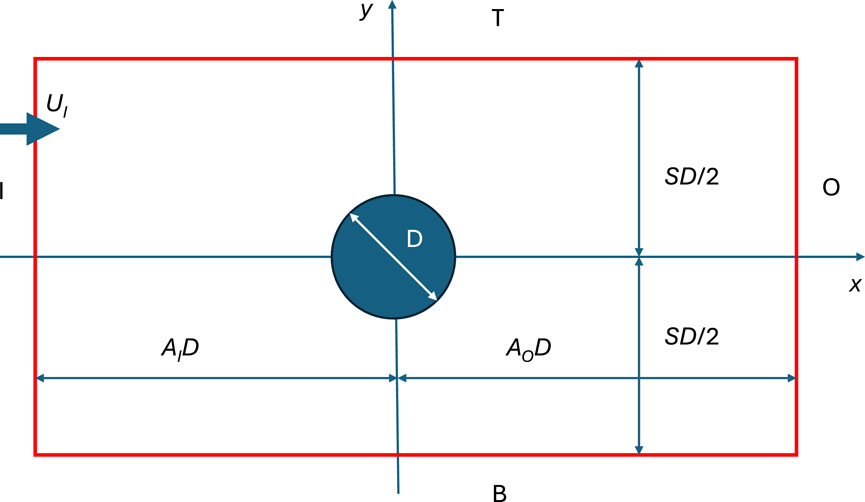
Figure 1. Control volume coinciding with the 2D rectangular computational domain for many vertical-axis turbine simulations. The flow is left to right, and the turbine of diameter $D$ is centered at the origin for $x$ and $y$. The inlet (I) is distance $A_{I}D$ from the turbine, and the top, T, and bottom boundary, B, are distance $SD/2$. $A_I$, the distance to the outlet, O, is not analysed here but is assumed to be large. All vorticity leaves the CV through O.

Many studies of isolated VATs, such as Balduzzi et al. (2016b), Balduzzi et al. (2016a), Rezaeiha et al. (2018), and Rezaeiha et al. (2019), and Tigabu et al. (2022) co-authored by the present first author, have used symmetric boundary conditions (SBCs) on T and B. These, in effect, turn the problem of an isolated VAT into one of an infinite cascade of alternatively counter-rotating, mirror-image VATs spaced $SD$ apart along the $y-$axis. It is important, therefore, to establish appropriate values of $S$ and $A_I$ that guarantee a negligible interaction between the turbines.

Some isolated VAT simulations have used a “slip” BC along T and B (e.g., Bangga et al., 2020; Lam and Peng, 2016). Since slip BCs like SBCs are “laterally-constrained,” thus preventing any flux of mass or momentum across T and B, the following analysis applies also to slip BCs.

In contrast, the interaction between a finite number, $N_t$, of turbines placed normal to the flow may be desired as a possible way of increasing the power extraction (Sun et al., 2021; Jiang et al., 2024). These studies use smaller values of $S$ than for “isolated” turbines with either SBCs if the turbines are counter-rotating or periodic BCs if they are co-rotating. Since the direction of the thrust is independent of the direction of rotation, the following analysis of SBCs also applies to periodic BCs. These laterally constrained BCs are appropriate for turbines in close proximity, but the interpretation of the results needs to be careful. It is often concluded that proximate VATs produce a higher power coefficient than isolated ones. We challenge this conclusion by demonstrating that the increase is more likely to be due to blockage caused by the BCs. Increases in power for interacting horizontal-axis turbines have also been claimed but also discounted for similar reasons to those developed here (Bleeg and Montavon, 2022). The present 2D geometry is simpler than the flow models for horizontal-axis turbines and yields specific equations for blockage effects.

Our study of four sets of BCs for (isolated) airfoil simulations at low incidence, and hence low drag, found a relation between the error in the drag and the lift and domain size for slip BCs (Golmirzaee and Wood, 2024). This was obtained from a curve fit to the numerical results for a wide range of domain sizes and slip BCs because no analytical expression for the error could be found. The most accurate BCs involved a point vortex to represent the airfoil lift, which corresponds to the side force on a turbine, whose necessity follows from the Kutta–Joukowsky equation (Thomas and Salas, 1986; Destarac, 2011). This makes the point vortex BC consistent with the equation for lift or side force; all other BCs tested were not. By “consistent with,” we mean that as the CV increases in size and the vorticity distribution around the airfoil surface shrinks to a point vortex, the BC should become more accurate, even though the velocity components are not prescribed for O.

We found, nevertheless, that the lift and drag coefficients obtained from any domain size were made more accurate by using the point vortex BC. This included domain sizes smaller than those used in current CFD practice, which are typically 30 times the chord. We did not, however, investigate the errors in the equation for the moment which becomes critical when moving from airfoils to VATs. Golmirzaee and Wood (2025) extended the airfoil study to high incidence by making the BCs also consistent with the drag, which is now significant. This is achieved by adding a point source BC to satisfy the relation between drag or thrust and source that was derived for incompressible flow by Lagally (1922) and Filon (1926). A point-vortex and point-source BC (PVSBC) was used by Kelmanson (1987) for low-Re studies of flow over a circular cylinder. Dannenhoffer (1987) applied it to the drag associated with shock waves in compressible flow. Allmaras et al. (2005) considered PS and PV components to their BCs for incompressible airfoil flow at a low $\alpha =12°$ where the drag is small. The PVSBC was the most accurate of all those we studied, in that it gives results for any domain size closer to those for an infinite domain than, say, slip and SBCs. Golmirzaee and Wood (2025) showed that the impulse form of the moment equation contains boundary integrals of the velocity, as in the lift equation, and an outlet integral involving the vorticity, as in the drag equation. That integral diverges logarithmically with distance from the airfoil, whereas the boundary integrals sum to zero for any distance and any location of the point source and vortex. It seems, therefore, that it is more difficult to devise boundary conditions that are consistent with the moment equation. Some of the consequences of this for VATs are discussed in Section 4. The airfoil simulations also showed that every BC gave accurate results for very large domains, and the errors caused by inconsistent BCs are generally impossible to quantify analytically.

The purpose of this study is to analyse some effects of slip, symmetry, and periodic BCs for isolated and proximate VAT simulation. For isolated turbines and airfoils, errors associated with BCs can be reduced simply by increasing the domain size. However, to our knowledge there is no available analysis that specifies the size necessary to achieve a prescribed accuracy. We show in the next section that current CFD practice for isolated VATs uses domain sizes that may not be sufficiently large for laterally constrained BCs to have negligible impact. For VATs in close proximity, laterally constrained BCs are appropriate, but our analysis shows that the inlet user-specified inlet velocity then becomes less than the freestream velocity, so the power and thrust coefficients are over-estimated.

The aim is to improve CFD accuracy and reduce computational cost by minimizing the required $S$ and $A_I$ for isolated turbine simulation. For constrained turbines where $S$ is fixed and laterally constrained BCs are appropriate, we provide corrections to the power and thrust coefficients and derive an equation for the minimum value of $A_I$ to achieve a specified accuracy. Using the impulse form of the thrust equation for a control volume (CV) that coincides with the outer boundaries, we derive in the next section the appropriate form of the Lagally–Filon equation for the source strength in steady flow as a function of the thrust, $T$, as a special case of the derivation by Golmirzaee and Wood (2025). This, in turn, provides for the first time an analytical expression of the effects of BCs on the power and thrust coefficients. Depending on the value of $S$, any non-zero $T$ makes $U_I$ smaller than the freestream velocity $U_{\infty }$, and the difference can lead to significant over-estimation of the power and thrust coefficients. We then derive the minimum $A_I$ required to achieve accurate simulations for any $S$ and thrust, $T$.

The problem under study is the 2D incompressible flow over a VAT for which

$•$ the CD shown in Figure 1 coincides with the CV;

$•$ the flow is steady, which in practice requires the number of blades, $N_b$, to be large enough for any cyclic variations in thrust and torque to be negligible;

$•$ $U_I$, the user-specified inlet axial velocity, is constant over I;

$•$ the top, T, and bottom, B, BCs are slip, symmetric, or periodic;

$•$ all the vorticity, $\mathrm{\Omega }$, exits through outlet O only;

$•$ $A_O$ is sufficiently large for the Neumann BC of zero normal gradient to be applicable for all velocities.

As with all CV analyses, the details of the turbine are not important. It is important, however, that an impulse analysis does not involve pressure, the absence of which is particularly useful in dealing with the thrust and moment. Pressure BCs are not under study.

There are several reasons to restrict the present study to 2D. The first two are as follows:

$•$ the analysis of BCs is easier in 2D as the computational domain has only four outer sides rather than six faces in three dimensions;

$•$ as noted above, many CFD analyses of VATs use a 2D domain.

The restriction to steady flow, which in practice requires a large blade count, is done for similar reasons. The unsteady impulse equations in 2D contain the time-derivative of an integral over the flow domain as well as a time-derivative of an integral over the body surface—see Equations (3.55) and (3.56) of Noca (1997). None of the studies we reviewed provided sufficient information about the flow field at each time step to evaluate these extra terms. In 3D, these unsteady integrals become volume integrals and are even harder to handle. The final reason to analyze 2D steady flow is to provide the first step in a comprehensive study of the effects of laterally constrained boundary conditions (BCs) on the computational fluid dynamics (CFD) analysis of vertical-axis turbines. We plan to extend the study to 2D unsteady flows followed by 3D unsteady flows but anticipate that these studies will require detailed results at each time step over the full domain.

The remainder of this study is organized as follows. The next section repeats the analysis of Golmirzaee and Wood (2025) to derive the relationship between $U_I$ and $U_{\infty }$ for VATs from a CV analysis of the thrust when the BCs prevent any flux of mass and momentum across the side walls. This gives corrections for VAT thrust and power. Section 3 applies the analysis and corrections to simulations of isolated and proximate VATs and derives lower limits on domain size for the former to guarantee a specified accuracy in the power and thrust. The common claim that stacking VATs normal to the flow in close proximity increases their power output is then disputed on the grounds that assuming $U_I=U_{\infty }$ causes the power coefficient to be overestimated when the thrust results in $U_I<U_{\infty }$. Section 4 discusses the CV equation for the moment and shows that BCs that are consistent with the thrust and side force equations by including a point source and vortex are still inconsistent with the moment equation. The significance of this inconsistency for VAT simulations is unknown. The final section provides a summary and lists the conclusions.

2 Boundary conditions and the thrust equation

The impulse form of the momentum equations for a body such as a turbine in steady flow is given by Golmirzaee and Wood (2024), who started with the fundamental equations (3.55) and (3.56) of Noca (1997). Equation 16 of Golmirzaee and Wood (2024) gives the airfoil drag derived using a square CV of sides 2$A$ centered on the body. If there is no normal velocity, $V$, in the incoming flow, the equation is easily modified to give $T$ for the CV in Figure 1 when slip, symmetry, or periodicity make the contributions from T and B sum to zero:

$\frac{T}{\rho }={\int }_I\left(U_{\infty }u+\frac{1}{2}{u}^2-\frac{1}{2}{v}^2\right)dy-{\int }_O\left[U_{\infty }u+\frac{1}{2}{u}^2-\frac{1}{2}{v}^2+y\left(U_{\infty }+u\right)\mathrm{\Omega }\right]dy,(1)$

where $\mathrm{\Omega }$ is the vorticity, which replaces the pressure appearing in the conventional CV equation for thrust. $u$ and $v$ are the perturbation velocities—that is, the departures from $U_{\infty }$ and zero, respectively. We decompose the first as $u=u_s+u_v$ where the subscript $s$ denotes the irrotational “source” contribution for reasons that will soon become apparent, and $v$ indicates the velocity due to the vorticity in the turbine wake. $u_v$ is non-zero (and generally negative) only in the wake at O, which is separated from the top and bottom boundaries by irrotational flow. The Neumann BC allows the approximation $\mathrm{\Omega }\approx -\partial u_v/\partial y$ and the $\mathrm{\Omega }$ integral in Equation 1 to be evaluated by parts. We note that the $U_{\infty }u$ and $U_{\infty }{u}_v$ terms in Equation 1 also appear in the equation for conservation of mass. Since $u=u_s$ at I and $u=u_s+u_v$ at O, we have

$-2{\bar{u}}_{s}S-{\int }_O{u}_{v}dy=0,(2)$

where ${\bar{u}}_s$, the average value of $u_s$, cannot change with distance from the turbine. If the quadratic terms like $v^2$ are negligible, Equation 1 reduces to

$\frac{T}{\rho }\approx -\left(U_I+{\bar{u}}_s\right){\int }_O{u}_{v}dy(3)$

where the differences between $u_s$ and ${\bar{u}}_s$ can also be ignored. Note that we have assumed ${\bar{u}}_s$ at I is equal and opposite ${\bar{u}}_s$ at O, otherwise the mass balance would force zero thrust. The common and key feature of Equations 2, 3 is the appearance of the outlet integral of $u_v$ in each which connects the equations for conservation of mass and axial momentum. Note that the connecting terms are all linear in $u_v$. This suggests that a cyclically varying $T$ for a VAT with finite $N_b$, when averaged over one cycle, would have the same relation with cyclic-average ${\bar{u}}_s$ as in Equation 3. In other words, cycle-averaging of $T$ and ${\bar{u}}_s$ would not distort the averages by producing the equivalent of Reynolds stresses which arise from averaging the nonlinear Navier–Stokes equations.

By Equation 2, the integral common to Equations 2, 3 is equivalent to the representation of the turbine as a source of fluid with strength $2{\bar{u}}_{s}S$. Thus, Equation 3 shows that the thrust (divided by density) is equal to the product of $U_I+{\bar{u}}_s$ and the strength of the source. As far as we know, this relationship between drag or thrust and an equivalent source in 2D flow was first derived by Lagally (1922) and can be viewed as a complement of the Kutta–Joukowsky equation relating to lift and vorticity (Li et al., 2015). The result was also derived, apparently independently, by Filon (1926) (who did not cite Lagally) (Liu et al., 2015) and without acknowledgement by Batchelor (1967)—see his Equation (5.12.15). Batchelor derived this equation from a CV analysis of a non-lifting body using the conventional momentum equation that includes pressure. He used a CV large enough for the quadratic terms to be negligible. His Figure 5.12.4 illustrates the outflow from the body that balances the inflow in the wake. Mokry (2016) gave a similar derivation of the Lagally–Filon drag equation and used it to correct drag measurements of model trucks in a wind tunnel.

If the velocities are normalized by $U_I$, the combination of Equations 2 and 3 gives the thrust coefficient $C_T^{*}=2T/(\rho U_I^{2}D)$ as

$C_T^{*}\approx 4\left(1+\frac{{\bar{u}}_s}{U_I}\right)\frac{{\bar{u}}_{s}S}{U_I}.(4)$

The positive root of Equation 4 gives

$\frac{{\bar{u}}_s}{U_I}\approx \frac{1}{2}\left(\sqrt{1+\frac{C_T^{*}}{S}}-1\right).(5)$

We emphasize that the average value of $u_s(x=-A_I,y)$ across I is independent of $A_I$ because slip, periodic, and SBCs prevent the spread of the source fluid out of T and B that would occur if a point source BC was applied at the side walls.

The role of ${\bar{u}}_s$ in VAT simulation does not seem to have been analysed previously. In all VAT studies we reviewed, including that by the present first author Tigabu et al. (2022), it was assumed that $U_I=U_{\infty }$. Deriving the thrust equation by allowing flow out of T and B for an isolated body, however, shows that the integral in Equation 3 is multiplied by $U_{\infty }$ (Golmirzaee and Wood, 2025). Thus,

$U_{\infty }=U_I+{\bar{u}}_s,(6)$

which means, for example, that the conventional thrust coefficient $C_T=2T/(\rho U_{\infty }^{2}D)$ is related to $C_T^{*}$ by

$\begin{array}{ll}\hfill C_T=C_T^{*}\frac{U_I^2}{U_{\infty }^2}\approx & 4C_T^{*}{\left(1+\sqrt{1+\frac{C_T^{*}}{S}}\right)}^{-2}\hfill \\ \hfill & =\frac{4S^2}{C_T^{*}}\left[2\left(1-\sqrt{1+\frac{C_T^{*}}{S}}\right)+\frac{C_T^{*}}{S}\right]\hfill \end{array}(7)$

using Equation 6, and, more importantly, that the correct power coefficient $C_P$ is related to that based on $U_I$ by

$C_P=C_P^{*}\frac{U_I^3}{U_{\infty }^3}\approx 8C_P^{*}{\left(1+\sqrt{1+\frac{C_T^{*}}{S}}\right)}^{-3}.(8)$

Golmirzaee and Wood (2025) suggested that corrections of the form of Equations 7, 8 be called “Lagally–Filon” corrections to honour the discoverers of the relationship between drag or thrust and source. Since Equation 5 can be evaluated using published values of $C_T^{*}$, Equations 7, 8 should be easily evaluated. Before doing that for some selected studies, two further points should be considered: the physical significance of non-zero $u_s$ and the requirements on $A_I$ to ensure that $u_s$, and hence $U_I$, can be assumed uniform at the inlet and outlet.

Consider a wind farm or hydrokinetic array comprising a finite number of turbines, $N_t$, along the $y-$axis, normal to the wind or water flowing at $U_{\infty }$ parallel to the $x-$axis. At distances that are large compared to $N_{t}SD$, the array or farm can be approximated as a single body with a thrust of approximately $N_{t}T$ where $T$ is the thrust of a turbine in a cascade. In 2D unbounded flow, $u_s$ due to $N_{t}T$ will eventually decay at the inverse distance from the turbines, so that $U_{\infty }$ is well-defined. A high-fidelity CFD analysis of all $N_t$ turbines, however, may not be feasible for a large CD using BCs consistent with the behaviour of $u_s$ at large distances. As an alternative for the turbine at the centre of the group at $y=0$, the domain in Figure 1 can be used with periodic or SBCs, provided that the blockage of the array or farm is accounted for by finding the difference between $U_I$ and $U_{\infty }$. Similar considerations of blockage apply if the CD of Figure 1 is used with SBCs for a supposedly isolated turbine.

Even though the average value of $u_s(x,y)$ is independent of $A_I$, its value determines the constancy of $u_s(x,y)$ across I and, therefore, the constancy of the inlet velocity. Thus, the $x-$dependence of $u_s(x,0)$ will be used to assess the choice of $A_I$. Each turbine can be replaced by a point source at $(0,iS)$ where $-\infty \le i\le \infty$ to give

$\frac{u_s\left(x,0\right)}{{\bar{u}}_s}=\frac{SD}{\pi }{\displaystyle \sum _{i=-\infty }^{\infty }}\frac{x}{x^2+{\left(iSD\right)}^2}=\coth \left(\pi \frac{x}{SD}\right)(9)$

where we note that a point vortex representation of the turbines will not contribute to $u_s(x,0)$. Using a typical value of $C_T^{*}=1.0$, Equation 5 gives ${\bar{u}}_s/U_I=0.01$ when $S=24.75$. For this $S$, Equation 9 requires $A_I/S=0.844$ or $A_I=20.9$ for $u_s(A_I,0)=1.01{\bar{u}}_s$. Note that a constant $u_s(x,0)$ implies $v(x,y)=0$ and a uniform $u_s(x,y)$. Since $\coth (\pi x/S)\to \pm 1$ as $x\to \pm \infty$, Equation 8 provides a consistency check on the assumption of constant ${\bar{u}}_s$ and the upstream value being equal and opposite to the downstream one. Furthermore, $A_O$ and $A_I$ should be comparable in size to ensure the validity of the outlet Neumann BC because coth (.) is an odd function. This check does not apply to $u_v$, so it is possible that $A_O$ must be larger than $A_I$ for the Neumann outlet condition to hold. Using the values of $A_I$ and $S$ that were just derived, Equation 7 shows that $C_T^{*}$ will differ from $C_T$ by approximately 2%, and $C_P^{*}$ from $C_P$ by 3% by Equation 8. Needless to say, this value of $S$ is larger and that of $A_I$ much larger than used in typical simulations.

Wind or water tunnel side walls can be represented by a slip BC. Thus, the analysis in this section relates to the assessment of blockage effects in measurements of VATs or other bodies, such as the truck models studied by Mokry (2016). These models were long relative to their cross-section dimensions so that the correction required placing singularities along the length of the model. As was found here, the result was a sometimes significant reduction in the drag coefficient. VAT experiments involve three-dimensional flow, and this may be the reason why their blockage corrections are more complex than the 2D results given here (e.g., Ross and Polagye, 2020). It is important to note that the present “correction” does not necessarily give the correct $C_T$ and $C_P$ for a VAT in an infinitely unbounded flow because it does not correct for the proximity of the side walls on the flow over the blades but only for the difference between $U_I$ and $U_{\infty }$. It is reasonable, however, to assume that $C_T$ and $C_P$ are close to their infinite domain values when $S$ is made large enough for $U_I$ to be close to $U_{\infty }$ and a small correction will be valid. The present analysis suggests that the choice of $S$ and $A_I$ should depend on $C_T^{*}$.

3 Application of thrust analysis

We consider two separate situations categorized by their different ranges of $S$. We start with isolated turbine studies at larger $S$ that use symmetry or slip-side wall conditions. The second case is multiple VATs, with emphasis on the performance when $S$ is lower than the typical values used for isolated VAT simulation. Since none of the studies of VATs in close proximity have considered the blockage effects analysed here, they are likely to have more errors than those for larger $S$.

3.1 Isolated turbines at larger $S$

The parameters from a selection of papers in the considerable literature on 2D simulations of VATs are shown in Table 1. In all cases, $N_b$ is low enough to cause significant unsteady effects related to the cyclic motion of the blades. Tigabu et al. (2022), co-authored by the first author here, studied the starting performance, so no steady, power-producing simulations were run. What is unexpected about the remaining entries in the table is the paucity of data on $C_T^{*}$, which is critical in assessing the effects of slip and SBCs. As shown above, if we choose $C_T^{*}=1.0$ as a typical value and neglect the effects of unsteadiness, then we need $S>25$ and $A_I>20$ for $U_I$ to be within 1% of $U_{\infty }$. Only Balduzzi et al. (2016a) and the larger domain studies of Balduzzi et al. (2016b) satisfy these restrictions. Given that $S$ can alter $C_T^{*}$ as well as make $U_I\ne U_{\infty }$ and that the choice of $A_I$ can have an indirect effect on $C_T^{*}$, we suggest that future numerical studies report the behavior of both $C_T^{*}$ and $U_I$ for a range of $A_I$ and $S$ before selecting values that do not significantly distort the results.

Table 1

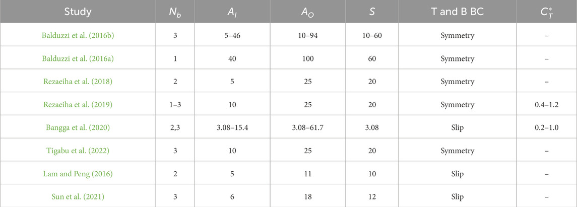
Table 1. Computational domains for 2D simulations of isolated VATs. All distances are in multiples of the turbine diameter. The slip BC for Bangga et al. (2020) refers to their fluent simulations which used the largest CD.

3.2 Multiple turbines at smaller $S$

We consider Sun et al. (2021) and Jiang et al. (2024) as examples of studies of groups of VATs aligned normal to the flow. Table 1 of Jiang et al. (2024) lists 17 previous studies of grouped VATs, of which the parameters in Table 2 are typical. $S_D$ in the table is the width of the CD which was held constant in both studies while $S$ was varied. This makes it possible only to provide a qualitative assessment of the effects of ${\bar{u}}_s$. $A_I$ and $A_O$ for Sun et al. (2021) were taken from their isolated turbine simulations as the values were not specified for the grouped turbines, but those in Table 2 appear consistent with the CD in their Figure 13 and with their Figure 12 if the velocity field is shown for the whole CD. In addition, the value of $S_D$ is estimated from Figure 13.

Table 2

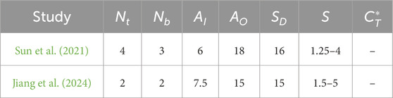
Table 2. Computational domains for two-dimensional simulations of multiple VATs. All distances are in multiples of the turbine diameter.

Figure 10 of Sun et al. (2021) shows the computed increase in $C_P^{*}$ averaged over the four turbines in the array for the range $1.25\le S\le 4$ for both co- and counter-rotating VATs. There is very little change in the average value of $C_P^{*}$ with the direction of rotation; at face value, this agrees with the present analysis. The results for $C_T^{*}$ were not reported, and their Table 4 shows considerable variation in the individual turbine power outputs, which is not surprising for a small $N_t$. The variation may well be due partly to a change in the individual $C_T^{*}$ and from the differences in the equation for SBCs and periodic BCs that are discussed in the next section. Nevertheless, an estimation of the effects of ${\bar{u}}_s$ is possible if $C_T^{*}=1$ is assumed for all turbines and we consider the smallest $S=1.25$; then, ${\bar{u}}_s/U_I=0.171$ from Equation 5, and Equation 8 gives $C_P/C_P^{*}=0.62$. In Sun et al. (2021), the increase in power output (given by the “efficiency” $\eta$ in the paper, which is equivalent to $C_P^{*}$) is a factor of 1.33, but we see that this is smaller than the estimated correction for the effects of ${\bar{u}}_s$ as $1.33\times 0.62=0.82<1$. In fact, correcting for ${\bar{u}}_s$ suggests a conclusion opposite to that of Sun et al. (2021)—turbines in close proximity produce less power individually than in isolation.

Table 10 of Jiang et al. (2024) shows that $C_T^{*}$ increases with decreasing $S$ without giving the values. Table 8 shows a maximum increase in $C_P^{*}$ at $S=1.5$ of 21%, whereas assuming $C_T^{*}=1.0$ gives ${\bar{u}}_s=0.145$, and so $C_P$ is reduced by 33% from $C_P^{*}$. We reach the same tentative conclusion that blockage effects actually reduce the power output of turbines in an array.

Our airfoil simulations with BCs that prevent outflow through the side walls show that the flow through O has ${\bar{u}}_s$ close to the value from Equation 5. This result suggests that it should be easy to tell whether a CFD simulation of a VAT or groups of VATs is compromised by a large value of ${\bar{u}}_s$.

4 Boundary conditions and the moment equation

Using a point vortex BC is consistent with the CV equation for lift or side force. Thomas and Salas (1986), Destarac (2011), Golmirzaee and Wood (2024), and Golmirzaee and Wood (2025) demonstrate that a point-source BC ensures consistency with the drag or thrust of an isolated turbine or body. We now consider the equation for the moment, $M$, or rotor torque which is critical for VATs. Its impulse form is given by Equation (A.2.7) of Siala (2019). Applied to the CV in Figure 1 and assuming that $U_I$ is constant, we have

$\begin{array}{ll}\hfill \frac{M}{\rho U_{\infty }}& =-{\int }_{I}uydy+{\int }_{T}uxdx+{\int }_{O}uydy-{\int }_{B}uxdx-A_I{\int }_{I}vdy-A_O{\int }_{O}vdy\hfill \\ \hfill & +\frac{S}{2}\left[{\int }_{T}vdx+{\int }_{B}vdx\right]+\frac{1}{2}{\int }_O\mathrm{\Omega }{y}^{2}dy\hfill \end{array}(10)$

where the quadratic terms, similar to those neglected in deriving Equation 3, are also neglected here. The contributions from T and B are included because the integrals multiplying $S/2$ are both zero for a cascade of counter-rotating turbines but their sum is not necessarily zero for a co-rotating cascade. This is the only difference between periodic and SBCs in the equations for axial $(T)$ and angular momentum $(M)$. This may be important in the further study of the differences in power output between arrays of co- and counter-rotating VATs.

If the CD is large enough for the velocities crossing all boundaries to be determined entirely by the point singularities, apart from the wake with non-zero $\mathrm{\Omega }$ and $u_v$, then the integrals in the first line and the square brackets on the second will sum to zero. This result holds for any location of the singularities, although it is reasonable to place both on the axis of rotation. The moment acting on the rotor or airfoil will then be given entirely by the vorticity term on the third line. In practice, however, the moment balance is likely to be more complex, with contributions from all terms, as suggested by the following analysis.

When the Neumman outlet BC is applicable, the vorticity term in Equation 10 can be rewritten as

$\frac{1}{2}{\int }_O\mathrm{\Omega }{y}^{2}dy\approx {\int }_O{u}_{v}ydy.(11)$

There are at least two ways that the vorticity term can be non-zero: the wake can be asymmetric about the point of minimum $u_v$, or a symmetric wake can have a trajectory away from the $x-$axis. To model an asymmetric and/or deflected wake, we assume

$u_v=u_m\left(1+B\left(y-y_m\right)\right)\exp \left[-A{\left(y-y_m\right)}^2\right](12)$

where $A$ and $B$ are scaling factors and $u_m$ is the value of $u_v$ at $y_m$, which can be of either sign, depending on the direction of rotation. $u_m$ is the minimum $u_v$ only if the asymmetric factor $B=0$. The exponential term is often used for symmetric wakes. It is the approximate, constant-eddy–viscosity solution to the Reynolds-averaged momentum equation for the wake, with $u_m$ and $y_m$ constrained by the constancy of the momentum flux due to $T$. This equation was assumed by Ouro and Lazennec (2021) and others for VAT wakes. Chapter 9 of Townsend (1976), for example, shows that turbulent flows are very sensitive to streamline curvature, so $y_m$ must remain small for Equation 12 to remain valid. The close similarity in behavior between a turbulent and laminar wake suggested the form of the asymmetric term. The $B-$term is consistent with the lowest-order symmetric term in Imai’s 1951 streamfunction for the deflected laminar wake behind a lifting body; see his Equation (11.3). Note that a symmetric streamfunction gives an asymmetric $u(y)$. It is also noted for later consideration that one of the symmetric terms in Imai’s equation has a coefficient proportional to the product of thrust and side force.

From Equations 3, 11, $T$ is given by

$\frac{T}{\rho }\approx -U_{\infty }{\int }_O{u}_{v}dy=U_{\infty }\sqrt{\frac{\pi }{A}}{u}_m,(13)$

using Equation 12, and so is independent of any asymmetry in Equation 12. Further analysis of the turbulence structure of the wake, such as Section 6.4 of Townsend (1976), requires $u_m\sim x^{-1/2}$, and $A\sim x^{-1}$ for the far-wake where $u_m$ is small and T in Equation 13 is constant. Both variations agree well with data for symmetric wakes, as shown by the zero pressure gradient data in Thomas and Liu (2004) and with the simulated airfoil wake in Golmirzaee and Wood (2025).

The vorticity term in the moment equation is proportional to

$-\left(\frac{B}{A}+y_m\right)\frac{T}{\rho U_{\infty }}(14)$

where the $y_m$ term comes solely from the symmetry and is not dependent on the particular form assumed in Equation 12. The width of the wake, $\delta$, will be controlled by the exponential term in Equation 12 and so $\delta \sim x^{1/2}$. This implies $B\sim x^{-1/2}$, and $B/A$ increases with $x$. Golmirzaee and Wood (2025) applied the analysis of Goldstein (1933) to estimate the contribution to the moment coefficient from the $y_m$ term in Equation 14. $y_m$ depends on the lift or side force generating a circulation in the wake. Denoting the symmetric component as $\mathrm{\Delta }{C}_M$, their estimate is

$\mathrm{\Delta }{C}_M\sim \frac{C_T{C}_S}{4\pi }\log \left(x/D\right)(15)$

where $C_S$ is the side force coefficient. Thus, the vorticity term will increase with $x$. Ouro and Lazennec (2021) used only the symmetric term in Equation 12, so it is possible that a deflected, symmetric far-wake is the most common for VATs or that an initially asymmetric wake becomes symmetric with increasing $x$. These possibilities are consistent with the approach to symmetry of the zero pressure gradient wake in Thomas and Liu (2004) and the development of an approximately symmetric but deflected wake measured out to 10$D$ along the midplane behind a VAWT by Peng et al. (2016). In contrast, Figure 6 of Huang et al. (2023) shows the wake asymmetry being maintained at least until $10D$. It is also noted that the asymmetry in the wakes measured by Huang et al. (2023) is not accurately modeled by Equation 12.

Nevertheless, Equation 15 can be used to assess the importance of $\mathrm{\Delta }{C}_M$, which may relate to the BCs needed for the accurate simulation of the torque. This is done by estimating the value of $x$ for which the vorticity integral is equal to the moment, using Equation 15 and the data in Table 3 of Huang et al. (2023) for the upwind turbine operating at a tip speed ratio of 4.5. For one case, $C_M=C_P/4.5=0.50/4.5$, $C_T=0.68$ and $C_S=0.02$. This gives a value of $x/D$ that is so large that the vorticity integral is unlikely to carry any significant moment out of the CD unless the asymmetry of the wake becomes dominant. For another case in their Table 3, $C_M=0.44/4.5$, $C_T=0.64$, and $C_S=0.34$. Thus $x/D=280$, which is also large enough to justify the same conclusion for practical simulations.

All possible wakes based on Equation 12 increase the magnitude of the vorticity term in the moment equation with $x$. This shows that the PSVBC is not consistent with a moment-generating VAT and that it is necessary to investigate changes to the boundary values of $u$ and $v$. These changes must not alter the circulation or the source strength, which would be inconsistent with the force balances. Golmirzaee and Wood (2025) showed the inconsistency of the PVSBC for an airfoil at $45°$, which has significant lift, drag, and moment, did not have an obvious effect on the computed moment; the changes in both forces and moment with changing domain size were very similar. Nevertheless, the critical importance of the moment for VATs suggests that a detailed study of the effect of domain size and BCs in the context of the moment equation is necessary.

5 Summary and conclusions

We have considered some aspects of the outer boundary conditions for the two-dimensional numerical simulation of vertical-axis turbines, both isolated and grouped normal to the flow.

For isolated turbines, the commonly used symmetry or slip conditions on the side walls prevent the outflow of fluid associated with the thrust on the turbine. This conclusion follows from an impulse analysis of the thrust in steady, incompressible flow. The outcome is a form of the Lagally–Filon equation relating drag or thrust to the strength of the source that represents the body or turbine. Commonly used boundary conditions for isolated turbines confine the outflow so that a component of the inlet velocity depends on the thrust and turbine spacing. This blockage makes the inlet velocity less than the freestream velocity at infinity. A correction for the difference in velocities was derived, which can be used to assess the adequacy of the domain size for a prescribed level of accuracy if “laterally-constrained” BCs are used. The Lagally–Filon equation implies that improved outer boundary conditions would include a point source term to ensure consistency with the thrust. The Kutta–Joukowsky equation requires a point vortex BC for consistency with the side force.

For turbines in close proximity, laterally constrained boundary conditions are appropriate, but the difference between the inlet and freestream velocities remains and is often significantly larger than for isolated turbines. Corrections are then required for the thrust and power coefficients based on the freestream velocity. In particular, it was shown that for closely spaced turbines aligned normally to the flow, the blockage correction may be sufficient to reverse the conclusions drawn in many studies that close proximity increases power output. In searching for examples with which to investigate the corrections for isolated and proximate turbines, it became apparent that the turbine thrust is rarely reported, and this made it impossible to reach firm conclusions about the blockage effects.

Point singularity boundary conditions that are consistent with the side force and thrust require the crucially important moment for a vertical-axis turbine to be balanced entirely by the vorticity in the wake behind the turbine. A simple model for the velocity distribution in the wake suggests that this is unlikely, and so the boundary conditions must be modified. It is recommended that a detailed study of the effects of domain size in conjunction with different boundary conditions be undertaken for an isolated vertical-axis turbine. It would be beneficial to start with a relatively large number of blades to approximate steady flow before considering the typical values of two or three.

To simplify its analysis, the study was restricted to two-dimensional steady flow because the two- and three-dimensional unsteady form of the impulse equations contain several extra terms, the evaluation of which was not possible from the published sources we used. The boundary condition involving the turbine as a source arises from the linear terms that connect the conservation of axial momentum to the conservation of mass. Linearity will ensure that the connection remains the same form when there are cyclic variations in the torque and flow. Thus, the cycle-average thrust will have the same relation to the cycle-average induced velocity as that between the steady thrust and induced velocity in Equations 2 and 3. Three dimensionality is more complicated, but it is likely that an application of quasi-two-dimensional impulse analysis will be useful; this is much like lifting-line theory for aircraft wings, in which the Kutta–Joukowsky equation is applied to each spanwise section of the flow. The forces acting in the direction of the rotational axis for vertical axis turbines are likely to be small, as are the spanwise forces for lifting-lines, so a similar sectional analysis is likely to be useful. These considerations suggest that the conclusions reached here from a two-dimensional, steady analysis have a wider generality than suggested by their fundamental assumptions.

One important turbine layout has not been considered in this study: multiple turbines separated in the direction of the flow rather than normal to it. The total thrust will be increased by axial stacking, and so a difference between $U_I$ and $U_{\infty }$ is likely unless a point source boundary condition is used, but it is more difficult to analyse. It seems reasonable to place the point sources and vortices at the axis of each turbine, with the consequence that the induced velocity for the array (at $-\infty$) will be due to the total thrust of the turbines and, therefore, very significant in general.

Data availability statement

The original contributions presented in the study are included in the article/supplementary material; further inquiries can be directed to the corresponding author.

Author contributions

DW: methodology, conceptualization, funding acquisition, and writing – original draft. NG: methodology, conceptualization, and writing – original draft.

Funding

The author(s) declare that financial support was received for the research and/or publication of this article. This work was supported by NSERC Discovery Grant RGPIN/04886-2017 and the Schulich endowment to the University of Calgary.

Conflict of interest

The authors declare that the research was conducted in the absence of any commercial or financial relationships that could be construed as a potential conflict of interest.

The authors declared that they were an editorial board member of Frontiers, at the time of submission. This had no impact on the peer review process and the final decision.

Generative AI statement

The author(s) declare that no Generative AI was used in the creation of this manuscript.

Publisher’s note

All claims expressed in this article are solely those of the authors and do not necessarily represent those of their affiliated organizations, or those of the publisher, the editors and the reviewers. Any product that may be evaluated in this article, or claim that may be made by its manufacturer, is not guaranteed or endorsed by the publisher.

References

Allmaras, S., Venkatakrishnan, V., and Johnson, F. (2005). “Farfield boundary conditions for 2-d airfoils,” in 17th AIAA computational fluid dynamics conference, 4711.

Google Scholar

Balduzzi, F., Bianchini, A., Ferrara, G., and Ferrari, L. (2016a). Dimensionless numbers for the assessment of mesh and timestep requirements in cfd simulations of darrieus wind turbines. Energy 97, 246–261. doi:10.1016/j.energy.2015.12.111

CrossRef Full Text | Google Scholar

Balduzzi, F., Bianchini, A., Maleci, R., Ferrara, G., and Ferrari, L. (2016b). Critical issues in the cfd simulation of darrieus wind turbines. Renew. Energy 85, 419–435. doi:10.1016/j.renene.2015.06.048

CrossRef Full Text | Google Scholar

Bangga, G., Dessoky, A., Wu, Z., Rogowski, K., and Hansen, M. O. (2020). Accuracy and consistency of cfd and engineering models for simulating vertical axis wind turbine loads. Energy 206, 118087. doi:10.1016/j.energy.2020.118087

CrossRef Full Text | Google Scholar

Batchelor, G. (1967). An introduction to fluid dynamics. Cambridge University Press.

Google Scholar

Bleeg, J., and Montavon, C. (2022). Blockage effects in a single row of wind turbines. J. Phys. Conf. Ser. 2265, 022001. doi:10.1088/1742-6596/2265/2/022001

CrossRef Full Text | Google Scholar

Dannenhoffer, J. F. (1987). Grid adaptation for complex two-dimensional transonic flows. Sc.D. thesis, Massachusetts Institute of Technology.

Google Scholar

Destarac, D. (2011). Spurious far-field-boundary induced drag in two-dimensional flow simulations. J. Aircr. 48, 1444–1455. doi:10.2514/1.c031331

CrossRef Full Text | Google Scholar

Filon, L. N. G. (1926). The forces on a cylinder in a stream of viscous fluid. Proc. R. Soc. Lond. Ser. A 113, 7–27. doi:10.1098/rspa.1926.0136

CrossRef Full Text | Google Scholar

Goldstein, S. (1933). On the two-dimensional steady flow of a viscous fluid behind a solid body. Proc. R. Soc. Lond. Ser. A 142, 545–562. doi:10.1098/rspa.1933.0187

CrossRef Full Text | Google Scholar

Golmirzaee, N., and Wood, D. H. (2024). Some effects of domain size and boundary conditions on the accuracy of airfoil simulations. Adv. Aerodynamics 6, 7–27. doi:10.1186/s42774-023-00163-z

PubMed Abstract | CrossRef Full Text | Google Scholar

Golmirzaee, N., and Wood, D. H. (2025). “Far-field boundary conditions for airfoil simulation at high incidence in steady, incompressible, two-dimensional flow to appear,” in Advances in aerodynamics. Available online at: http://arxiv.org/abs/2411.13077.

Google Scholar

Huang, M., Sciacchitano, A., and Ferreira, C. (2023). Experimental and numerical study of the wake deflections of scaled vertical axis wind turbine models. J. Phys. Conf. Ser. 2505, 012019. doi:10.1088/1742-6596/2505/1/012019

CrossRef Full Text | Google Scholar

Imai, I. (1951). On the asymptotic behaviour of viscous fluid flow at a great distance from a cylindrical body, with special reference to filon’s paradox. Proc. R. Soc. Lond. Ser. A. Math. Phys. Sci. 208, 487–516.

Google Scholar

Jiang, J., Xie, D., Zhao, M., and Zheng, X. (2024). The study on the load and flow field of a twin-rotor vertical axis tidal current turbine. Ships Offshore Struct. 19, 2150–2163. doi:10.1080/17445302.2024.2329018

CrossRef Full Text | Google Scholar

Kelmanson, M. (1987). A direct boundary integral equation formulation for the oseen flow past a two-dimensional cylinder of arbitrary cross-section. Acta Mech. 68, 99–119. doi:10.1007/bf01190877

CrossRef Full Text | Google Scholar

Lagally, M. (1922). Berechnung der Kräfte und Momente, die strömende Flüssigkeiten auf ihre Begrenzung ausüben. ZAMM-Journal Appl. Math. Mechanics/Zeitschrift für Angewandte Math. und Mech. 2, 409–422. doi:10.1002/zamm.19220020601

CrossRef Full Text | Google Scholar

Lam, H., and Peng, H. (2016). Study of wake characteristics of a vertical axis wind turbine by two- and three-dimensional computational fluid dynamics simulations. Renew. Energy 90, 386–398. doi:10.1016/j.renene.2016.01.011

CrossRef Full Text | Google Scholar

Li, J., Bai, C.-Y., and Wu, Z.-N. (2015). A two-dimensional multibody integral approach for forces in inviscid flow with free vortices and vortex production. J. Fluids Eng. 137, 021205. doi:10.1115/1.4028595

CrossRef Full Text | Google Scholar

Liu, L., Zhu, J., and Wu, J. (2015). Lift and drag in two-dimensional steady viscous and compressible flow. J. Fluid Mech. 784, 304–341. doi:10.1017/jfm.2015.584

CrossRef Full Text | Google Scholar

Mokry, M. (2016). Lagally force on an automotive model in a solid-wall wind tunnel. Tech. Rep. SAE Technical Paper. doi:10.4271/2016-01-1622

CrossRef Full Text | Google Scholar

Noca, F. (1997). On the evaluation of time-dependent fluid-dynamic forces on bluff bodies. California Institute of Technology. Ph.D. Thesis. doi:10.7907/K2Z0-9016

CrossRef Full Text | Google Scholar

Ouro, P., and Lazennec, M. (2021). Theoretical modelling of the three-dimensional wake of vertical axis turbines. Flow 1, E3. doi:10.1017/flo.2021.4

CrossRef Full Text | Google Scholar

Peng, H., Lam, H., and Lee, C. (2016). Investigation into the wake aerodynamics of a five-straight-bladed vertical axis wind turbine by wind tunnel tests. J. wind Eng. industrial Aerodynamics 155, 23–35. doi:10.1016/j.jweia.2016.05.003

CrossRef Full Text | Google Scholar

Rezaeiha, A., Montazeri, H., and Blocken, B. (2018). Towards accurate cfd simulations of vertical axis wind turbines at different tip speed ratios and solidities: guidelines for azimuthal increment, domain size and convergence. Energy Convers. Manag. 156, 301–316. doi:10.1016/j.enconman.2017.11.026

CrossRef Full Text | Google Scholar

Rezaeiha, A., Montazeri, H., and Blocken, B. (2019). On the accuracy of turbulence models for cfd simulations of vertical axis wind turbines. Energy 180, 838–857. doi:10.1016/j.energy.2019.05.053

CrossRef Full Text | Google Scholar

Ross, H., and Polagye, B. (2020). An experimental assessment of analytical blockage corrections for turbines. Renew. Energy 152, 1328–1341. doi:10.1016/j.renene.2020.01.135

CrossRef Full Text | Google Scholar

Siala, F. F. (2019). Experimental investigations of the unsteady aerodynamics of oscillating airfoils operating in the energy harvesting regime. Ph.D. thesis, Oregon State University.

Google Scholar

Sun, K., Ji, R., Zhang, J., Li, Y., and Wang, B. (2021). Investigations on the hydrodynamic interference of the multi-rotor vertical axis tidal current turbine. Renew. Energy 169, 752–764. doi:10.1016/j.renene.2021.01.055

CrossRef Full Text | Google Scholar

Thomas, F. O., and Liu, X. (2004). An experimental investigation of symmetric and asymmetric turbulent wake development in pressure gradient. Phys. Fluids 16, 1725–1745. doi:10.1063/1.1687410

CrossRef Full Text | Google Scholar

Thomas, J. L., and Salas, M. (1986). Far-field boundary conditions for transonic lifting solutions to theeuler equations. AIAA J. 24, 1074–1080. doi:10.2514/3.9394

CrossRef Full Text | Google Scholar

Tigabu, M. T., Khalid, M. S. U., Wood, D., and Admasu, B. T. (2022). Some effects of turbine inertia on the starting performance of vertical-axis hydrokinetic turbine. Ocean. Eng. 252, 111143. doi:10.1016/j.oceaneng.2022.111143

CrossRef Full Text | Google Scholar

Townsend, A. (1976). The structure of turbulent shear flow. Cambridge University Press.

Google Scholar

Nomenclature

$\mathit{A}$ scaling factor, Equation 12

${\mathit{A}}_{\mathit{I}}$ distance from the inlet to turbine in multiples of $D$, Figure 1

${\mathit{A}}_{\mathit{O}}$ distance from the turbine to outlet in multiples of $D$, Figure 1

B bottom of the computational domain, Figure 1

$\mathit{B}$ scaling factor, Equation 12

${\mathit{C}}_{\mathit{M}}$ turbine moment coefficient

${\mathit{C}}_{\mathit{P}}$ turbine power coefficient

${\mathit{C}}_{\mathit{P}*}$ turbine power coefficient based on $U_I$

${\mathit{C}}_{\mathit{S}}$ turbine side force coefficient

${\mathit{C}}_{\mathit{T}}$ turbine thrust coefficient

${\mathit{C}}_{\mathit{T}*}$ turbine thrust coefficient based on $U_I$

$\mathit{D}$ turbine diameter

I inlet of the computational domain, Figure 1

$\mathit{M}$ turbine moment

${\mathit{N}}_{\mathit{b}}$ number of blades in a vertical-axis turbine

${\mathit{N}}_{\mathit{t}}$ number of turbines in a stack

O outlet of the computational domain, Figure 1

$\mathit{S}$ width of the computational domain in multiples of $D$, Figure 1

${\mathit{S}}_{\mathit{D}}$ width of the computational domain for a stack of turbines in multiples of $D$, Section 3.2

T top of the computational domain, Figure 1

$\mathit{T}$ turbine thrust

${\mathit{U}}_{\mathit{I}}$ streamwise velocity at the inlet

${\mathit{U}}_{\infty }$ freestream velocity

$\mathit{u},\mathit{v}$ perturbation velocities due to the turbine in $x-$ and $y-$directions respectively

${\mathit{u}}_{\mathit{m}}$ value of $u_v$ at $y_m$ in the wake

${\mathit{u}}_{\mathit{s}}$ $u$ due to the turbine as a source

${\mathit{u}}_{\mathit{v}}$ $u$ due to the vorticity in the wake

$\mathit{x},\mathit{y}$ streamwise and normal co-ordinates, respectively

${\mathit{y}}_{\mathit{m}}$ location of minimum wake velocity

$\mathit{\rho }$ air density

$\mathbf{\Omega }$ vorticity Overlines denote average values at any $x$