 Costas A. Varotsos
 Vladimir F. Krapivin
 Vladimir Y. Soldatov2
- 1Laboratory of Upper Air/UoAthens Climate Research Group, Department of Environmental Physics and Meteorology, Faculty of Physics, University of Athens, Athens, Greece
- 2Institute of Radioengineering and Electronics, Russian Academy of Sciences, Moscow, Russia
The issues of air pollution are inextricably linked to the mechanisms underlying the physicochemical functioning of the biosphere which together with the atmosphere, the cryosphere, the lithosphere, and the hydrosphere constitute the climate system. We herewith present a review of the achievements and unresolved problems concerning the modeling of the biochemical cycles of basic chemicals of the climate system, such as carbon and nitrogen. Although the achievements in this area can roughly describe the carbon and nitrogen cycles, serious problems still remain associated with the accuracy and precision of the processes and assessments employed in the relevant modeling.
Modeling Schemes of the Global Carbon Cycle
It is generally recognized today that the complete understanding of the CO2 contribution in the formation of the atmospheric greenhouse effect presupposes a thorough examination of the biogeochemical dynamics of the carbon cycle (Kondratyev and Varotsos, 1995; Kondratyev et al., 2004; Krapivin and Varotsos, 2008; Amann et al., 2011). In the current literature a lot of schematic pathways of carbon cycle are considered in the form of global CO2 changes. Herewith we refer to the most important ones, demonstrating their main characteristics in order to understand the limits of the simulation of the carbon cycle compounds. It should be worthwhile to note that all the assumed pathways of the CO2 cycle on a global scale are often separated into two groups, notably: point wise (averaged on a global scale) and spatial (averaged on a local scale). All these schematic pathways consider that the biosphere is consisting of three ecosystems, viz., atmosphere, oceans, and land. In addition, a number of the available schematic diagrams of the carbon cycle distinguish the organic from inorganic types (Kondratyev et al., 2004). Moreover, the temporal averaging of all carbon processes and reservoirs is often performed on an annual basis, and thus the atmosphere is regarded as an homogeneous medium (point-wise). In this investigation the World Ocean and the surface ecosystems are based on global data bases for the carbon reservoirs. In general, these diagrams describe the atmospheric CO2 concentrations assuming a typical scenario for the anthropogenic activity (Krapivin and Varotsos, 2008).
Most of the modeling estimates of the basic components of the carbon cycle show that its maximum supply is concentrated in the World Ocean and its minimum in the atmosphere. It should be stressed, however, that the natural processes that determine the global carbon cycle dynamics obey various time scales. For example, the amounts of the dead organic matter that is buried in the the oceans bottom, exhibit temporal scales of the order of 102–103 years, while the biological components of the carbon cycle on land, appear a temporal variability of several decades. Consequently, the consideration of the above-mentioned temporal variability of the biospheric carbon cycle is of great importance. Keeping this in mind in the relevant modeling, it is equally important to consider the temporal variability of the complete atmospheric mixing that can last up to a couple of years (Kondratyev et al., 2004).
Additionally the spatial variability in the atmospheric CO2 concentrations is of crucial importance. Routine observations obtained at different stations revealed that the CO2 field appears substantial discrepancies in the annual variability. More specifically, the amplitude of the CO2 variation ranges from 10 ppm over Antarctica to 10–15 ppm at the near Arctic region. This heterogeneity is attributed to the presence of large vegetation communities in the northern hemisphere (NH) which exhibits substantial seasonal photosynthesis (Kondratyev et al., 2004).
In this context, the latitudinal distribution of CO2 in the atmosphere displays non-linear character (Varotsos, 2005; Varotsos and Kirk-Davidoff, 2006; Varotsos et al., 2012, 2013). The increased CO2 content in the atmosphere of the NH is closely linked to both the direct CO2 anthropogenic emissions and the vegetation cover. For instance, it is considered that the organic fuel burning results in almost 90% of the total emissions of carbon which is located in the latitudinal belt 30°N–60°N (Kondratyev et al., 2004).
As previously stated, an important component of the well-known schematic pathways of the carbon cycle on a global basis is the distribution of carbon fluxes into the World Ocean. In this connection, there is now the required information to select several oceanic layers in various depths to distinguish the spatial heterogeneities. In this regard, most of the relevant studies assume two or three layers in the vertical structure of the oceans considering both the photic and deep layers. More recent schemes of the global carbon cycle take into account all the above-mentioned heterogeneities, increasing thus considerably the fidelity of the relevant modeling algorithms. Two of the widely used schematic pathways are shown in Figures 1, 2 (Kondratyev et al., 2004).
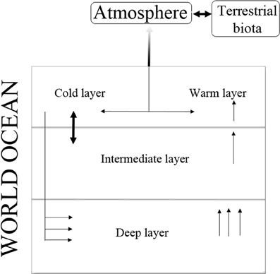
Figure 1. Schematic pathways of the carbon fluxes in the modeling algorithms that consider various depths in the World Ocean.
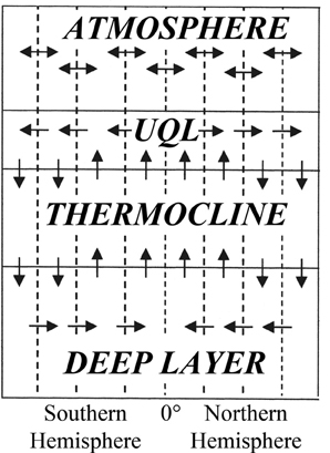
Figure 2. Schematic pathways of the circulation in the World Ocean for the mapping of carbon cycles considering the upper quasi-homogeneous layer (UQL).
As mentioned above, the process of exchange of CO2 in the atmosphere-ocean borders reveals the contribution of the World Ocean to the global cycle of CO2. The extent of this exchange is expressed by the dynamic characteristics of the turbulent layers of water and air near the interface of the ocean and the atmosphere. In this context, numerous physical schemes take into account the sea wave formation, as well as formation of foam and various films. Specifically, these schemes consider that CO2 either dissolves into the ocean releasing the CO2 that is required for photosynthesis, or enters the atmosphere. The cause of this twofold process in the atmosphere-ocean boundary is the relative difference between the partial pressures of CO2 dissolved in the water and that of contained within the atmosphere. Indeed, this oriented CO2 transport at the frontier “air-water” is much more complex and therefore its investigation postulates expensive in-field campaigns and a detailed classification of both synoptic and geographical conditions of the oceans surface (Ayers, 2005; Krapivin and Varotsos, 2008).
In the study of the global carbon cycles the emphasis is placed on the role of the surface ecosystems. In the process of photosynthesis, plants absorb CO2 and, conversely, the decomposion of dead plants causes the emission of CO2 into the atmosphere. Thus, between the living and dead organic matter of the land biosphere and the atmosphere a continuous exchange of CO2 is taking place. Many conceptual schematic diagrams illustrate this exchange and serve as background for modeling algorithms of the global carbon cycle. Figures 3, 4 show two examples of such diagrams (Kondratyev et al., 2004).
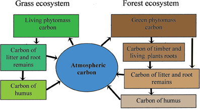
Figure 3. The flow-chart of the carbon fluxes interplay in the system atmosphere-plant-soil with the grass and forest ecosystems.
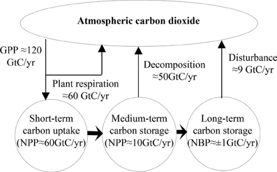
Figure 4. The scheme of the global carbon cycle (GPP, gross primary productivity; NPP, net primary productivity; NEP, net ecosystem productivity; NBP, net biome productivity; GtC, gigatons of carbon = 109 metric tones of C).
Of course, the correct assessment of the carbon fluxes in the terrestrial biosphere involves both the detailed quantization of the types of soil-plant formations and the correct assessment of the parameterization of the biocenotic processes. For this approach, the knowledge of the following parameters would be available: areas of vegetation and soils, data of the vital functions of soil microorganisms, and technologies of an operational monitoring of landscapes. However, the accurate figures about the details of the soil-plant formations are not available so far, and therefore the current accuracy of the estimates of carbon fluxes is poor (Kondratyev et al., 2004).
To overcome this difficulty, a modeling scheme of carbon cycle is required, which would describe the ranking of the important biospheric components and the possible pathways of transformation of carbon. As an example, an indicative schematic diagram of carbon flux for the required modeling assessment is given in Figure 5 and in Table 1. The employment of this model allows numerical experiments for the optimal spatial quantization, considering comparative estimates of the constituents involved and thus to successively approach required quantization (Kondratyev et al., 2004).
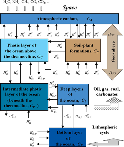
Figure 5. The block-diagram of the CO2 cycle considering the global biogeochemical processes in the atmosphere-land-ocean system. The corresponding details about CO2 are given in Table 1 (Kondratyev et al., 2006).
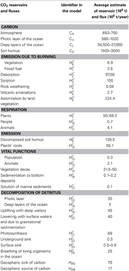
Table 1. Model of global CO2 cycle (MGCDC): Carbon reservoirs and fluxes and their average estimates considering the global processes illustrated in Figure 5 (Kondratyev et al., 2006).
Modeling Schemes of the Nitrogen Cycle in Nature
It is a truism that nitrogen is one of the basic nutrient elements in nature. That is why its global cycle is of great interest. According to the current understanding its cycle exhibits a composit structure of several processes of its compounds that are mainly formed due to water migration and plethora of relevant atmospheric processes (Varotsos et al., 1998; Akimoto, 2003; Wilson et al., 2007; Van der A et al., 2008; Tzanis et al., 2009, 2011; Xue et al., 2010). The known nitrogen cycle is subject to intense anthropogenic forcings generated by the interaction of the nitrogen cycle both directly and through the influence on the related processes (Krapivin and Varotsos, 2008). Therefore, the development of a reliable model of the nitrogen cycle in nature should be based on the consideration of the whole complex natural processes and those initiated by human activities. Figures 6, 7 illustrate a schematic pattern of the main supplies and fluxes of nitrogen.
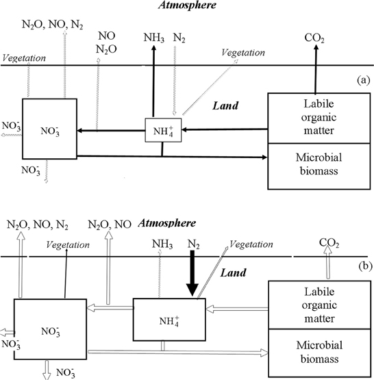
Figure 6. Block-diagram of biogeochemical cycles of C and N in the water-limited ecosystems (Krapivin and Varotsos, 2008). (A) Dry season; (B) wet season.
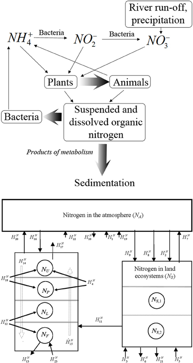
Figure 7. The scheme of nitrogen fluxes in marine medium (top) and in nature (Table 2) (bottom).
It is generally recognized that the natural sources of nitrogen oxides are strongly related to bacteria, volcanic eruptions, and several atmospheric phenomena, like the lightning discharges. More specifically, the biogeochemical cycle of nitrogen includes among others, fixation, mineralization, nitrification, assimilation, and dissimilation mechanisms that have been investigated in many studies (e.g., Krapivin and Varotsos, 2008). Their complexity is determined by the rates of transformation of the nitrogen compounds their supplies, etc.
It is well-known that nitrogen participates in the biospheric processes with a complex structure of fluxes that are characterized by a hierarchical sequence of cycles in the biosphere. For example, starting from the atmosphere, nitrogen enters the microorganisms, migrating successively to soil, higher plants, animals, and humans. Then nitrogen returns back to the soil due to the death of living organisms. From the soil nitrogen, is either consumed by plants and living organisms or is emitted into the atmosphere. Approximately the same pattern is observed in the hydrosphere. The feature of the above-mentioned cycles is their openness to the available nitrogen removal processes from the biospheric balance into rocks, from which returns much slower. Given the nature of the nitrogen cycle in the biosphere and its reservoir structure, it is quite possible to formulate a global scheme of nitrogen fluxes (Krapivin and Kelley, 2009).
To simplify the scheme of the calculation of nitrogen fluxes presented in Figure 7 (bottom), the advection processes in the balance equations of nitrogen cycle can be illustrated by a superposition of the fluxes HN14 and HN15. However, for the development of such a model by employing these equations several corrections are necessary. Therefore, the estimates of the fluxes HNi given in Table 2 for their consideration in the GIMS should be corrected following this criterion. Detailed description of the nitrogen cycle as unit of the GIMS was given by Krapivin and Varotsos (2008).
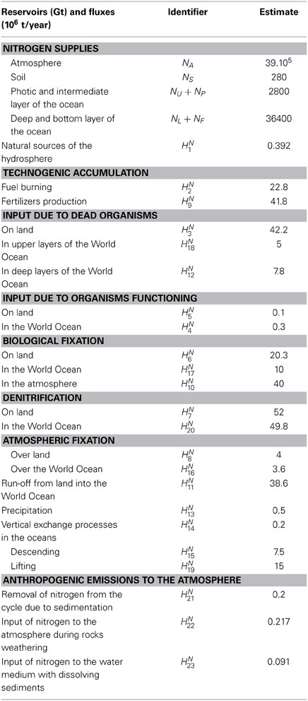
Table 2. Characteristics of reservoirs and fluxes of nitrogen in the biosphere (Figure 7 bottom).
Conclusions
The problem of reliable modeling of biochemical cycles that control greenhouse effect, bioproductivity and environmental quality, is far from being solved. The correlations between biochemical cycles and the many activities of human society show that a deeper knowledge of the mechanisms involved must be obtained especially through the observational data of the biochemical processes. In this connection, the reliable assessment of the role that the biochemical cycles play in global ecodynamics is crucial considering that these are the main indicators of sustainable development (Kondratyev et al., 1995, 2006; Nitu et al., 2013a,b). As an example, in the formation of the carbon cycle the soil-plants and the World Ocean play a crucial role which may be assessed by the global carbon cycle model. This model considers different scenarios with geographical grids greater than the needed ones for a reliable assessment.
Conflict of Interest Statement
The authors declare that the research was conducted in the absence of any commercial or financial relationships that could be construed as a potential conflict of interest.
References
Akimoto, H. (2003). Global air quality and pollution. Science 302, 1716–1719. doi: 10.1126/science.1092666
Amann, M., Bertok, I., Borken-Kleefeld, J., Cofala, J., Heyes, C., Höglund-Isaksson, L., et al. (2011). Cost-effective control of air quality and greenhouse gases in Europe: modeling and policy applications. Environ. Model. Software 26, 1489–1501. doi: 10.1016/j.envsoft.2011.07.012
Ayers, G. (2005). Air pollution and climate change: has air pollution suppressed rainfall over Australia? Clean Air Environ. Qual. 39, 51.
Kondratyev, K. Y., Krapivin, V. F., Savinykh, V. P., and Varotsos, C. A. (2004). Global Ecodynamic: A Multidimensional Analysis. Chichester: Springer/Praxis. doi: 10.1007/978-3-642-18636-3
Kondratyev, K. Y., Krapivin, V. F., and Varotsos, C. A. (2006). Natural Disasters as Interactive Components of Global Ecodynamics. Chichester: Springer/Praxis.
Kondratyev, K. Y., Pokrovsky, O. M., and Varotsos, C. A. (1995). Atmospheric ozone trends and other factors of surface ultraviolet radiation variability. Environ. Conserv. 22, 259–261. doi: 10.1017/S0376892900010663
Kondratyev, K. Y., and Varotsos, C. (1995). Atmospheric greenhouse effect in the context of global climate change. Il Nuovo Cimento C, 18, 123–151. doi: 10.1007/BF02512015
Krapivin, V. F., and Kelley, J. J. (2009). “Model-based method for the assessment of global change in the nature—society system,” in Global Climatology and Ecodynamics eds A. P. Cracknell, V. Krapivin, and C. Varotsos (Chichester: Springer Praxis), 133–183.
Krapivin, V. F., and Varotsos, C. A. (2008). Biogeochemical Cycles in Globalization and Sustainable Development. Chichester: Springer/Praxis.
Nitu, C., Krapivin, V. F., Soldatov, V. Y., and Dobrescu, A. (2013a). “A device to measure the geophysical and hydrophysical parameters,” in Proceedings of the 19th International Conference on Control Systems and Computer Science - CSCS19 (Bucharest), 281–284.
Nitu, C., Krapivin, V. F., Varotsos, C. A., Cracknell, A. P., Soldatov, V. Y., and Dumitrascu, A. (2013b). “An effective tool for the tropical cyclones monitoring,” in Proceedings of the 19th International Conference on Control Systems and Computer Science -CSCS19 (Bucharest), 276–280.
Tzanis, C., Varotsos, C., Christodoulakis, J., Tidblad, J., Ferm, M., Ionescu, A., et al. (2011). On the corrosion and soiling effects on materials by air pollution in Athens, Greece. Atmos. Chem. Phys. 11, 12039–12048. doi: 10.5194/acp-11-12039-2011
Tzanis, C., Varotsos, C., Ferm, M., Christodoulakis, J., Assimakopoulos, M. N., and Efthymiou, C. (2009). Nitric acid and particulate matter measurements at Athens, Greece, in connection with corrosion studies. Atmos. Chem. Phys. 9, 8309–8316. doi: 10.5194/acp-9-8309-2009
Van der A, R. J., Eskes, H. J., Boersma, K. F., van Noije, T. P. C., Van Roozendael, M., De Smedt, I., et al. (2008). Trends, seasonal variability and dominant NOx source derived from a ten year record of NO2 measured from space. J. Geoph. Res. 113, D04302. doi: 10.1029/2007JD009021
Varotsos, C. (2005). Power-law correlations in column ozone over Antarctica. Int. J. Rem. Sens. 26, 3333–3342. doi: 10.1080/01431160500076111
Varotsos, C. A., Chronopoulos, G. J., Cracknell, A. P., Johnson, B. E., Katsambas, A., and Philippou, A. (1998). Total ozone and solar ultraviolet radiation, as derived from satellite and ground-based instrumentation at Dundee, Scotland. Int. J. Rem. Sens. 19, 3301–3305. doi: 10.1080/014311698213984
Varotsos, C. A., Melnikova, I., Efstathiou, M. N., and Tzanis, C. (2013). 1/f noise in the UV solar spectral irradiance. Theor. Appl. Clim. 111, 641–648. doi: 10.1007/s00704-012-0697-8
Varotsos, C., and Kirk-Davidoff, D. (2006). Long-memory processes in ozone and temperature variations at the region 60 S-60 N. Atmos. Chem. Phys. 6, 4093–4100. doi: 10.5194/acp-6-4093-2006
Varotsos, C., Ondov, J., Tzanis, C., Öztürk, F., Nelson, M., Ke, H., et al. (2012). An observational study of the atmospheric ultra-fine particle dynamics. Atmos. Environ. 59, 312–319. doi: 10.1016/j.atmosenv.2012.05.015
Wilson, N., Edwards, R., Maher, A., Näthe, J., and Jalali, R. (2007). National smoke free law in New Zealand improves air quality inside bars, pubs and restaurants. BMC Public Health 7:85. doi: 10.1186/1471-2458-7-85
Keywords: biochemical processes, carbon cycle, nitrogen cycle, modeling, greenhouse effect
Citation: Varotsos CA, Krapivin VF and Soldatov VY (2014) Modeling the carbon and nitrogen cycles. Front. Environ. Sci. 2:8. doi: 10.3389/fenvs.2014.00008
Received: 25 February 2014; Paper pending published: 17 March 2014;
Accepted: 03 April 2014; Published online: 23 April 2014.
Edited by:
Yong Xue, London Metropolitan University, UKReviewed by:
Eleni Drakaki, National Technical University of Athens, GreeceDeepak Jhajharia, North Eastern Regional Institute of Science and Technology, India
Copyright © 2014 Varotsos, Krapivin and Soldatov. This is an open-access article distributed under the terms of the Creative Commons Attribution License (CC BY). The use, distribution or reproduction in other forums is permitted, provided the original author(s) or licensor are credited and that the original publication in this journal is cited, in accordance with accepted academic practice. No use, distribution or reproduction is permitted which does not comply with these terms.
*Correspondence: Costas A. Varotsos, Laboratory of Upper Air/UoAthens Climate Research Group, Department of Environmental Physics and Meteorology, Faculty of Physics, University of Athens, University Campus, Bldg. Phys 5, Athens 15784, Greece e-mail:Y292YXJAcGh5cy51b2EuZ3I=