From daily climatic scenarios to hourly atmospheric forcing fields to force Soil-Vegetation-Atmosphere transfer models

This paper presents a method to produce long term climatic forcing fields to force Soil-Vegetation-Atmosphere transfer (SVAT) models in off-line mode. The objective is to increase the temporal frequency of existent climate projections databases from daily frequency to hourly time step to be used in impact climate studies. A statistical clustering k-means method is used. A tens of clusters seems to be enough to describe the climate variability in term of wind regimes, precipitation and thermal and humidity amplitude. These clusters are identified in the future projections of climate and reconstructed sequences at hourly frequency are obtained for all the forcing variables needed by a SVAT model, typically: air temperature, specific humidity, wind speed and direction, precipitation, direct short-wave radiation, downward long-wave radiation, and scattered short-wave radiation. Eleven years of observations from two sites in France are used to illustrate the method: the Chartres station (Paris) and Blagnac station (Toulouse). The reconstruction algorithm is able to produce diurnal cycles that fits well with hourly series from observations (1998–2008; 1961–1990) and from climatic scenarios (1961–2100). The diurnal amplitude and mean value is well represented for variables with marked daily cycle as temperature or humidity. Changes in the mean wind direction are represented and, to a certain extent, changes in wind intensity are also retained. The mean precipitation is conserved during the day even if the method is not able to reproduce the short rain picks variability. Precipitation is used as input in the clusterization process so in clusters representative of rainy days some diurnal variability is nevertheless retained.

Introduction

Investigations on climate change impact often requires projections of climate at the local scale to be used to force a Soil-Vegetation-Atmosphere transfer (SVAT) model¹ in offline mode. The easier way to obtain long term databases for the atmospheric parameters used to force SVAT models, would be to directly² use climate simulations from General Circulation Models or Regional Climate Models when those datasets are available with a high temporal frequency (1–3 h). Due to computational storage limitations, often this product is only available over a restricted area, during short periods of time and emission or land use scenarios available are limited. One example is the study of Tanaka et al. (2006) that estimates the impact on hydrological variables of the Seyhan River basin, Turkey, through off-line simulations for the periods 1994–2003 and 2070–2080.

Future climate projections databases currently available for the whole Europe area that includes different emission scenarios and an ensemble of models have daily frequency, as PRUDENCE (http://prudence.dmi.dk/), ENSEMBLES (http://www.ensembles-eu.org/), or those from the Climatic Research Unit of the New Anglia University (http://www.cru.uea.ac.uk/cru/data/hrg/). This means that, for a grid point, only the daily mean or at the best the maximum and minimum values are available. In this case, an increase in the temporal frequency of the variables from daily to hourly time step is needed.

One way to do that is to obtain relationships between large scale circulation patterns and local variables through a classification based on atmospheric circulations or weather types. This classification is determined in a high resolution hourly reanalysis database and projected in to a daily database of climate scenarios. These climate scenarios are then reconstructed at high temporal frequency using mean (or a representative) diurnal cycles from the same weather types in the reanalysis database (see Huth et al., 2008 for a deep review of this method). This approach was used by Quintana-Seguí et al. (2010, 2011), Querguiner et al. (2012) and during the RexHySS project (Ducharne et al., 2009) to study the impact of climate change on some French basins. Recently it was used by Lemonsu et al. (2012) to study climate change impact over Paris region and by Déqué et al. (2011) for mountainous zones.

This approach has two limitations: first it needs a previous large scale weather type classification at synoptic scale. This kind of product is not available everywhere and it demands high amount of data and validation time. It is only after a recent COST action 733 (Philipp et al., 2010) that were developed for the European regions tools to simply overview of the existing circulation classification catalogs. The second limitation is that the method, as applied in the studies cited before, cannot produce extremes higher than those observed during the period used to construct the weather type classification.

The methodology presented here allows to generate climatic input databases, based on past near surface observations, for SVAT models that need high-resolution atmospheric forcing inputs. In fact, observational data at hourly frequency is available from the operational network of surface stations with large coverage around the world (http://worldweather.wmo.int/). The idea here is to use single-site observations from a sufficiently long period (so all the diversity of weather types affecting the site will be represented) and apply a cluster analysis using only the mean, maximum, and minimum daily data, that are the only one available for modeled future scenarios, to classify the data in function of the type of the diurnal cycle for each variable.

These mean meteorological characteristics are identified in the future projections of climate from Regional Climate Models. A cluster number is then attributed and a reconstructed sequence for the future projections at hourly frequency is obtained. Figure 1 represent the flux diagram of the algorithm and describes the methodology.

FIGURE 1

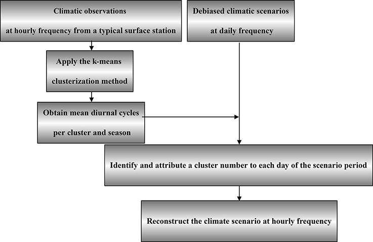
Figure 1. Flux diagram of the algorithm: from hourly frequency observations and daily climatic scenarios to reconstructed climate scenarios at hourly frequency.

Two sites are selected to prove the feasibility of the method. The Chartres station close to Paris and Blagnac station close to Toulouse were used to perform a k-means cluster classification for the construction period 1998–2008 (Section Materials and Methods). A validation analysis is performed for reconstructed series for the construction period and the climatic reference period 1961–1990. Near-surface atmospheric outputs from seven Regional Climate Models from the EU-FP6 ENSEMBLES (Hewitt, 2005) are reconstructed at hourly frequency from 1961 to 2100 and the method is validated using hourly climate projections provided by the Marx-Planck-Institute (Section Results). The statistics are shown for both areas in Section Materials and Methods but to limit the number of figures and, as the objective of the paper, is to illustrate the methodology, the results of validation and application to climatic scenarios in Section Results are shown only for Paris area. Nevertheless, a complete documentation of results, figures, and analyses of the types of diurnal cycles for both sites can be found, in French, on Hidalgo (2012a,b).

Materials and Methods

Hourly Climatic Data from a Typical Meteorological Station

Data from two meteorological stations are used due to specific needs on projections of climate at the local scale on two French National projects on climate change impact on Paris [MUSCADE (http://www.cnrm.meteo.fr/ville.climat/spip.php?article85)] and Toulouse [ACCLIMAT (http://www.cnrm.meteo.fr/ville.climat/spip.php?rubrique47)] areas. Air temperature, specific humidity, wind speed and direction and precipitation from the operational network of Meteo-France were extracted from: Blagnac station (Toulouse) located at (43°′12″N, 1°22′42″E). This station is situated over grass inside the airport at 6 km in the North-West of Toulouse city and from Chartres station (Paris) situated also over grass at 155 m over the sea level at (48°27′ 36″N, 1°30′00″E) at 80 km at the South-West of Paris. As far as possible, it is convenient to use observations from meteorological stations representative of rural areas because scenarios of climate change do not consider the influences of urban areas on their own local climates.

Statistical Method

The statistical k-means method is applied for the construction period (1998–2008, 4018 days) to obtain a set of clusters that represents the plurality of weather situations representative of Paris and Toulouse local climates. To define the cluster structure the following variables are used, the daily: diurnal thermal amplitude (ΔT, °C), mean wind speed (ff, m s⁻¹) and direction [dd (four quadrants were defined for the 1–90; 91–180; 181–270 and 271–360 wind direction)], mean precipitation (pp, mm), and mean specific humidity (q, gr kg⁻¹). In the method the distance measure determines how the similarity of two elements is calculated when forming the clusters. Here the Euclidean distance is used. To avoid differences in scale among the variables the standard deviation is used to normalize their values.

An important question that needs to be tackled before applying the k-means clustering algorithm is how many clusters (k) are in the dataset. This is not known a priori and often the strategy is to perform an iterative exercise increasing the number of clusters. There are different means to evaluate the resulting clustering quality in a quantitative manner (He et al., 2002). For us the objective is to obtain the best reconstructed series for all variables once the attribution method is applied. Two parameters are used to evaluate the resulting series. The first represents how well the resulting mean diurnal cycles from clusters serves to identify and attribute a cluster number for a particular day. In others words, for the construction period, the frequency distribution of clusters issue from the attribution process is evaluated against those obtained directly from the k-means clustering method. The second one is the multivariate Root Mean Square Error of the reconstructed and original observed series. The magnitudes evaluated are the hourly near surface temperature, relative humidity, wind u-v components and precipitation from observations.

Figure 2 shows the mean frequency deviation (solid line) and the mean RMSE (broken line) for 10³ repetitions of the iterative exercise where k increase from 4 to 25 clusters. In both locations Paris and Toulouse, the frequency deviation increase (solid line) and the RMSE decrease (broken line) when k increases. The reason is that a high number of clusters results in mean diurnal cycles of temperature, humidity, wind, and precipitation that could be very similar for some seasons resulting in a degradation in the inter-cluster separation making difficult the cluster attribution process.

FIGURE 2

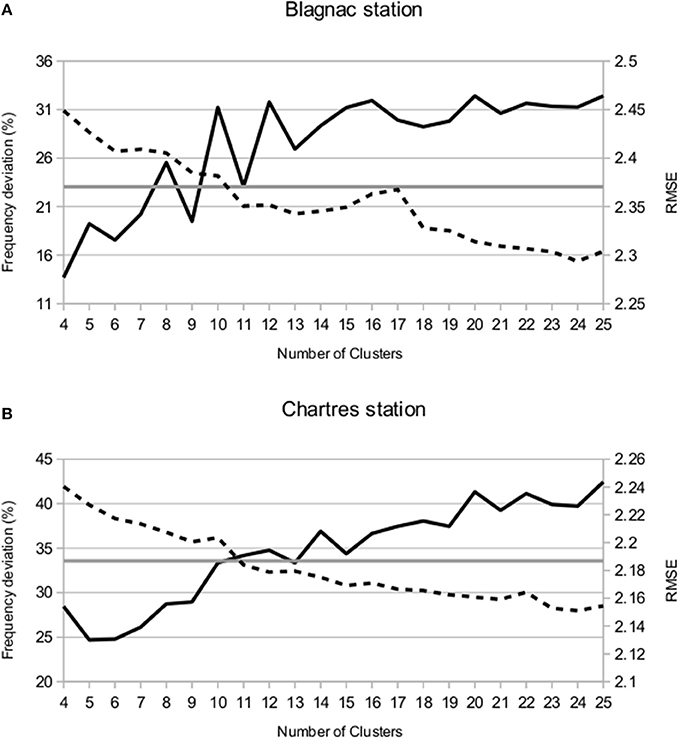
Figure 2. Mean frequency deviation (solid line), multivariate RMSE (broken line), and the maximum acceptable degradation value for frequency deviation (gray line) in the cluster assignation process for Paris (A) and Toulouse (B) sites when cluster number (k) increase from 4 to 25.

The choice of an optimal number of clusters is here done as follows. The range (Freq_max − Freq_min) is calculated. A threshold of 50% of this quantity is fixed as a maximum acceptable degradation in the cluster assignation process (gray line in Figure 2). The number of clusters that produces relative Freq_min values under this threshold are identified. For this cluster numbers, RMSE is computed. The number of clusters relative to the minimum RMSE is kept. For Paris and Toulouse, thresholds are 33.56 and 23.05% respectively. Two relative minimums at k = 5 and 9 are identified for Paris and three at k = 6, 9, and 11 for Toulouse. RMSE is minimum at k = 9 and k = 11 for Paris and Toulouse respectively. Nine and eleven clusters are respectively retained as an optimum number for the cluster analysis and further development.

Types of Diurnal Cycles from Clusters

Table 1 summarizes the values of centroids for each variable. Those are the values that characterize each type of day obtained from the clustering process for Paris (nine clusters) and Toulouse (11 clusters) respectively. They will be used to classify days in periods outside of the construction period 1998–2008 [as explained in Section First validation: cluster attribution and hourly reconstruction for the construction period (1998–2008)]. Figure 3 presents the occurrence frequency (number of days belonging to a cluster) in total percentage and per season.

TABLE 1

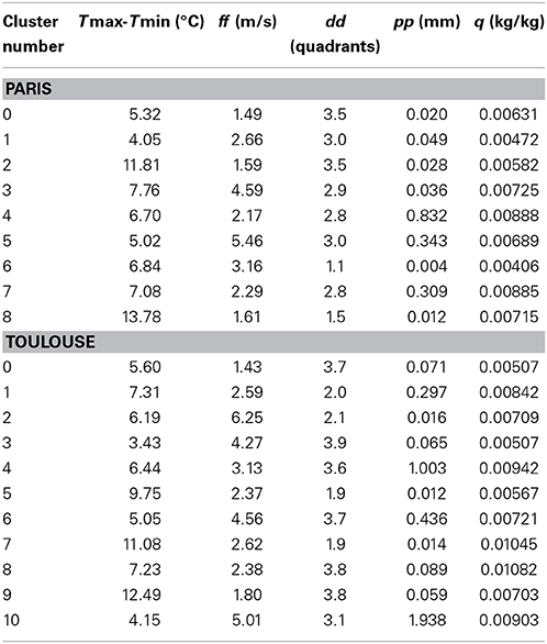
Table 1. Values for the clusters centroids of the diurnal amplitude of air temperature and daily mean values for wind speed, wind direction (expressed in quadrants for wind direction inside of the following ranges 1–90; 91–180; 181–270; and 271–360 wind direction), precipitation, and specific humidity.

FIGURE 3

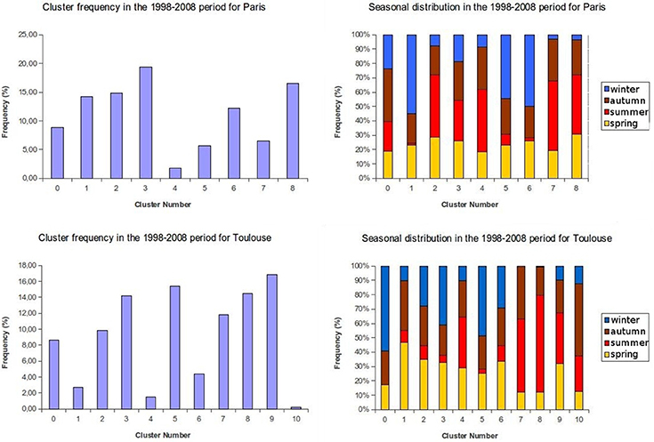
Figure 3. Occurrence frequency in total percentage (left) and its distribution per season (right).

In Paris region predominant winds flow from the south-west (mainly in winter and autumn, clusters 1, 3, 5, and 7) and the north and north-east (mainly in winter and summer, clusters 6 and 8). Humid winds from the west are also frequents (clusters 0 and 2). Winds from south and south-east (cluster 4) are infrequent and normally it corresponds to temporary phases before a perturbation. Even if the clusters are present in almost all seasons, predominant winter clusters are 1, 5, and 6 and summertime clusters are 2, 4, and 7. The mean daily thermal amplitude varies between 4°C (for cluster 1) and 13°C (for cluster 8) and the daily amplitude in relative humidity varies between 5 and 50%. Precipitation is concentrated on clusters 4, 5, and 7 for all seasons.

In Toulouse dominant winds are, in descending order of importance, the humid westerly wind from the Atlantic Ocean [represented here by clusters 0, 3, 4, 6, 8, 9 (the more frequent), and 10], moderate south-easterly wind (cluster 1 and 7) that can be very strong (called the Autan wind, cluster 2) and finally the southerly wind (cluster 5). Predominant winter clusters are 0, 3, and 5. Representative summertime clusters are 7, 8, and 9. The daily thermal amplitude varies between 3 and 12°C and the daily amplitude in relative humidity between 10 and 50%. Precipitation is concentrated on clusters 1, 4, 6, and 10.

Seasonal intra-cluster differences in the mean hourly cycles where found for both, Paris and Toulouse locations. Some are related to the large-scale seasonal forcing as for example the seasonal delay in the daybreak or a higher thermal amplitude for warm seasons that for the cold ones. For example cluster 6 for Paris (Figure 4A) presents a high thermal amplitude variability 5°C in winter and 10°C in summer. In consequence the same relation is found for the relative humidity. Even though, the rest of variables for this cluster (the precipitation rate, the wind speed and wind direction) are very consistent between seasons. Other are related to differences in the circulations at the synoptic scale. For example again in Paris, hourly mean temperature for cluster 4 (Figure 4B), decrease during winter days from 10°C in the morning to 5°C in the afternoon. This type of day corresponds to a low pressure (985 hpa) situation with quasi-constant relative humidity (98%) and stronger winds during the morning (4.5 m s⁻¹ instead 2–3 m/s for other seasons). In Toulouse, cluster 10 (Figure 4C) corresponds to rainy days. In Winter (blue line) this situation describes days with south westerly winds and storms during the afternoon (15–20 h UTC). This type of day has temperatures around 10°C and very low thermal amplitude. Humidity increase during the day (q = 0.006 to 0.008 kg kg⁻1) being the atmosphere close to saturation at the end of the afternoon (Hu = 99%).

FIGURE 4

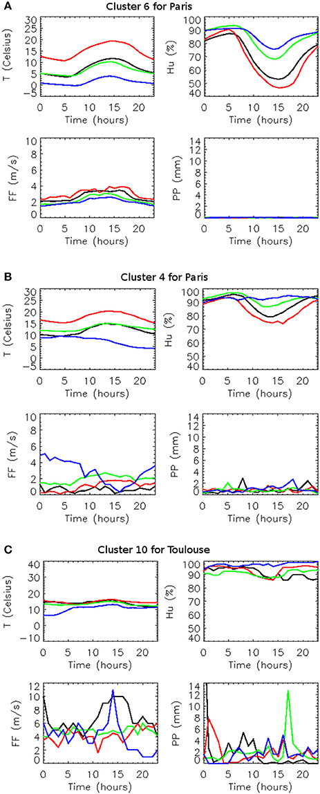
Figure 4. Mean diurnal cycles of temperature, relative humidity, wind speed and precipitation for Paris (A,B), and Toulouse (C). Seasonal intra-clusters differences for spring, summer, autumn, and winter are in black, red, green, and blue lines respectively.

Results

First Validation: Cluster Attribution and Hourly Reconstruction for the Construction Period (1998–2008)

The cluster methodology aims to represent the climatic variability of a site using a finite set of daily mean cycles. For that, a cluster number is associated by the k-means method to each day of the period and a series that maintains the climatic features and variability of the site can be directly reconstructed using the seasonal diurnal mean cycles associated to each cluster (hereafter direct method). When working with an alternative period in the past (observations or model outputs) or in the future (model outputs) where the clustering process is not possible, it is necessary to attribute a type of day (cluster number) to each day of the alternative period.

The attribution method is here based on variables that are available at daily frequency in climate scenarios databases: the mean, max, and min values for temperature and relative humidity; the daily mean values of u-v wind components and precipitation.

These values are obtained for the construction period. The deviation between those values for a day of the alternative series and from each cluster is computed and summed for each cluster (S_K). All the data is normalized with its standard deviation. The cluster number with the minimum value of S_K is attributed to the day.

A hourly reconstructed series is obtained for all the observables using the observed mean daily value and the shape of the cluster diurnal cycle for the season of this particular day. For temperature and relative humidity, maximum and minimum values are available so the shape amplitude of the cluster diurnal cycle is modulated as follows:

$\begin{array}{l}T{(h)}_i=\overline{T_i}+{(\Delta T{(h)}_{season\_mean})}_k{}^{\ast }Cte\hfill \\ Cte=\frac{{(T_{\max }-T_{\min })}_{obs}}{{(T_{\max }-T_{\min })}_k}\hfill \end{array}$

Where i is the day number and k the cluster number. T_max and T_min are the maximum and minimum values of the observed (or modelized) field. For a cluster k, ΔT(h)_{season_mean} is the seasonal mean hourly cycle of ΔT(h) being ΔT(h) = T(h)_j −T(h)_j. Over all days (j) of the season.

The performance of the attribution method to produce hourly reconstructed series close to observations is presented and discussed in next section where the method is applied to the WMO reference climate period 1961–1990.

We want to focus here on the differences found on the occurrence frequency when the reconstruction is performed using the direct method and the attribution method.

When analyzing the number of days affected to each cluster number for both methods, differences between 0.02 and 7.7% for Toulouse and 0.2 and 8.7% for Paris are found resulting in a total of 24 and 30% of the days that are affected to an annex cluster. Most of those differences are concentrated in summer and autumn. This is due to the fact that for each cluster four seasonal hourly cycles are obtained. Some, for the same season, are very similar so the method is not able to attribute the exact cluster number. This has not a big impact on the reconstructed series because the method attributes a mean cycle very close to the original one (Figures 5, 6), one must be prudent exploring changes in the frequency of the clusters occurrence in future projections because this may be an artifact of the attribution methodology.

FIGURE 5

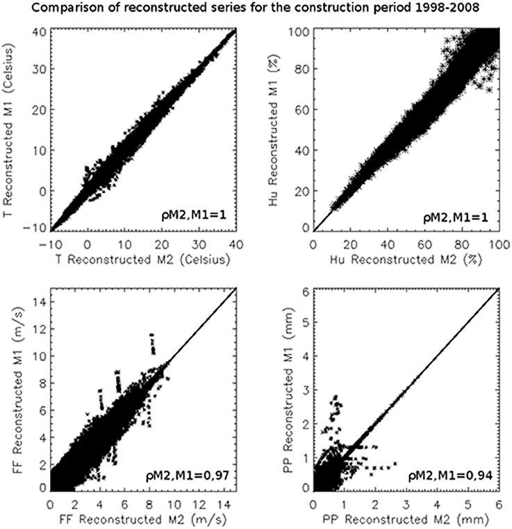
Figure 5. Scatter plot and linear Pearson correlation coefficient of the 1998–2008 reconstructed series directly from the statistical process (direct method, M1) and reconstructed series after attribution process (attribution method, M2) over Paris for hourly air temperature, relative humidity, wind speed, and precipitation.

FIGURE 6

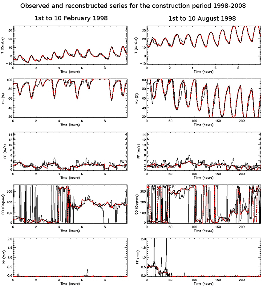
Figure 6. Temporal evolution for wintertime (left, 1st to 10 February 1998) and summertime (right, 1st to 10 August 1998). In simple-line, observations from Chartres station (Paris), in black and red bold, hourly reconstructed series directly from the statistical process (direct method, M1) and reconstructed series after attribution process (attribution method, M2) respectively.

Second Validation: Applying the Attribution Method to an Alternative Observational Period

The objective here is to show the feasibility of the method for an alternative period in the past where the clustering process is not possible and attribution of a cluster number is mandatory. The attribution method is applied for the WMO reference climate period 1961–1990 where at Chartres (Paris) and Blagnac (Toulouse) locations three-hourly observations are available.

Values of the mean, max and min values for temperature and relative humidity; the daily mean values of u-v wind components and precipitation are obtained from the 1961–1990 three-hourly observed series after a spline function reconstruction that provides hourly disaggregation.

The hourly reconstructed 1961–1990 series are compared to observations of Chartres station by means of the scatter-plot and the linear Pearson correlation coefficient (represented by ρ_x,y in the figures) (Figure 7) and the temporal evolution of each variable (Figure 8, a random period of 10 consecutive days in summer and winter is shown). The reconstruction algorithm is able to produce diurnal cycles that fits well with observations during different seasons. The diurnal amplitude and mean value is well represented for variables with marked daily cycle as temperature (ρ_x,y = 0.97) or relative humidity (ρ_x,y = 0.91). For temperature, there is a jump in the intersection between 2 days that is more or less pronounced in function of the cycle features⁴, for example during the night from 7th to 8th August (Figure 8). Changes in the mean wind direction are well represented and, to a certain extent, changes in wind intensity are also retained (ρ_x,y = 0.76). The mean precipitation is conserved during the day but the method is not able to reproduce the short rain picks variability (ρ_x,y = 0.52). However precipitation is used as input in the clusterization process and some variability is retained in clusters that are representative of rainy days. For example days of autumn with precipitation during the late afternoon (Figure 4C, cluster 10 for Toulouse, green line).

FIGURE 7

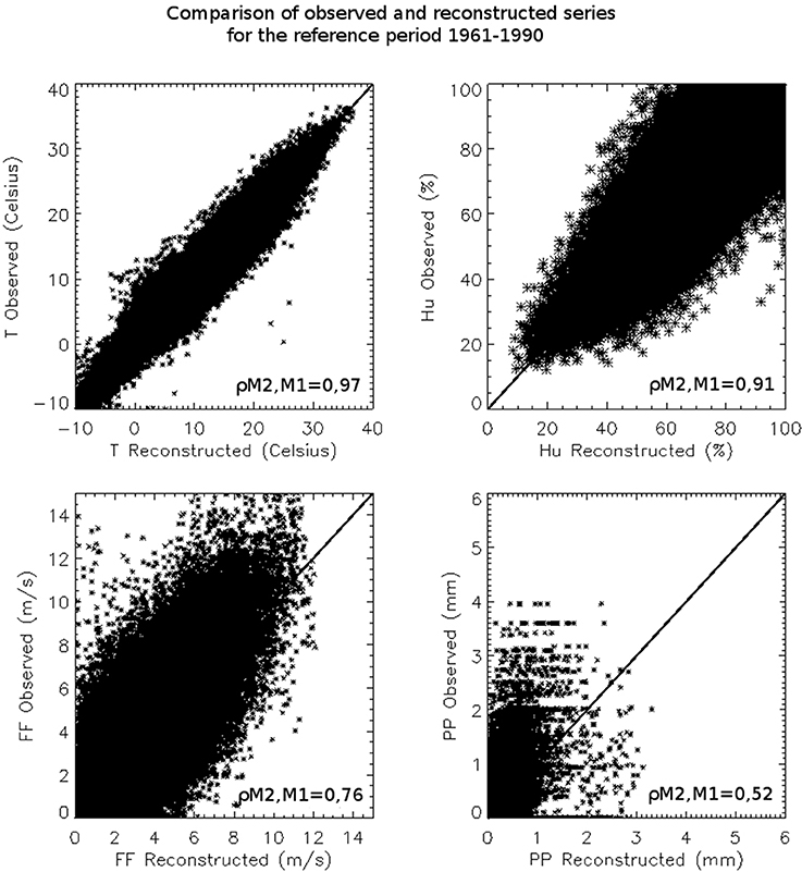
Figure 7. Scatter plot and linear Pearson correlation coefficient of the 1961–1990 observed and reconstructed series after attribution process over Paris for hourly air temperature, relative humidity, wind speed, and precipitation.

FIGURE 8

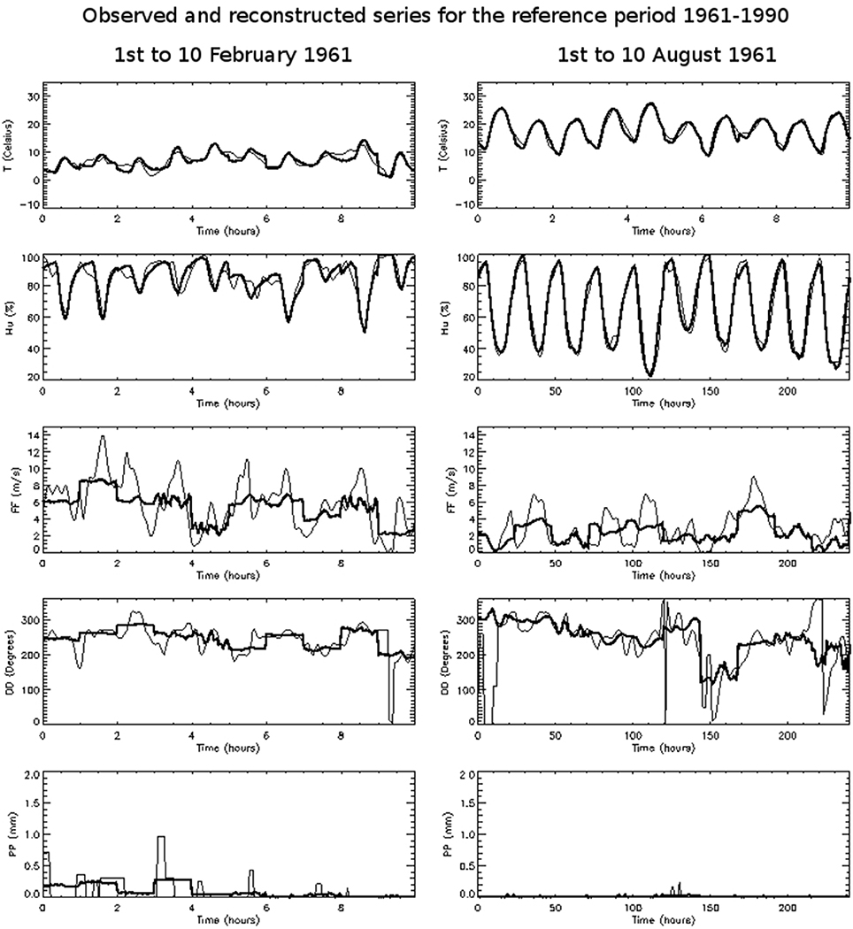
Figure 8. Temporal evolution for wintertime (left, 1st to 10 February 1961) and summertime (right, 1st to 10 August 1961). In simple-line observations from Chartres station (Paris) and in bold hourly reconstructed series after attribution process.

Validation and Application to Climate Scenarios from Regional Climate Models Simulations

To explore the applicability of the method to future scenarios, the Climate Service Center of the Max Planck Institute for Meteorology provided for validation time-series at the nearest grid point for near-surface hourly temperature, specific humidity, u- and v-velocities, net surface solar radiation and downward, long-wave radiation from REMO simulations.

Three kinds of simulations were available in function of the emission scenario (Nakicenovic et al., 2000): A1B, B1, and E1. A common control period run (1961–2000) was performed for A1B and B1 scenarios and a single one for E1 scenario. Three projections from 2001 to 2100 were performed for A1B and B1 and from 2001 to 2099 for E1 scenario.

Systematic errors from Global and Regional Climate models are too large to allow for direct use of the outputs in the attribution process so a previous bias correction using observed climate data during a control period (1961–1990) is performed before to apply the attribution methodology. Here this bias is calculated in base to the percentile differences between the mean daily value for modeled and observed series during the reference period as explained in Gonzalez-Aparicio and Hidalgo (2012). This technique, uses a correction function that restores model percentiles in present time to those from observations. This means that it is supposed that the model is able to reproduce the distribution of climatic variables but not their exact value of the percentile. The strongest hypothesis of the method is to consider that model errors are stationary so that it is possible to use the correction function for future projections. Once the mean daily value is corrected the diurnal cycle is reproduced using the original hourly anomaly to the original mean value.

Afterwards, hourly reconstructed series for the three future projections are obtained for all the variables as explained in Section First validation: cluster attribution and hourly reconstruction for the construction period (1998–2008). Precipitation was not available in this database so this variable was not used as a prescriptor in the attribution process. The application of the attribution method to climate projections is possible assuming that under future climate conditions the occurrence frequencies of clusters might be modified but their dynamical characteristics remain unchanged. It is the same hypothesis as for methodologies based on weather classes and this approach is supported by studies as those from Corti et al. (1999) and Stone et al. (2001) which suggested that anthropogenic climate change may manifest itself as a projection onto the pre-existing natural modes of variability of the climate system (Najac et al., 2011).

Figure 9 shows the performance of the methodology to reconstruct 10 consecutive days in February and August 2061 for the A1B scenario for Paris. In this case reconstruction for surface solar radiation (RG) and downward, long-wave radiation (RA) is shown. The methodology to calculate and reconstruct the temporal series for the radiative variables is explained in Appendix 1 in Supplementary Material. It could be seen that the daily maximum value of RG is slightly underestimated in reconstructed series but the cycle conserves the integral sum over the day. The linear Pearson correlation coefficient is calculated for a 30 years window (2061–2090) to maintain the statistical significance of comparison with values obtained for the reference period. Table 2 shows that the performance of the method is very similar for the three simulations A1B, B1, and E1. The impact of leaving out precipitation from the attribution process seems to have more impact over the wind speed reconstruction that over other variables. The score for linear Pearson correlation coefficient for the wind speed is lower (ρ_x,y varies from 0.30 to 032 in function of the scenario) than for the reference period (ρ_x,y = 0.76). This is due to an underestimation of wind gusts mainly in the ranges of 7–10 m s⁻¹.

FIGURE 9

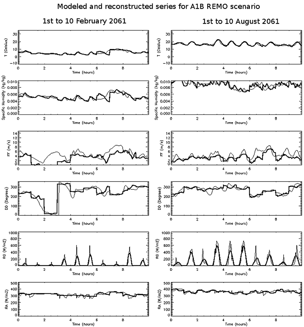
Figure 9. Temporal evolution for wintertime (left, 1st to 10 February 2061) and summertime (right, 1st to 10 August 2061). In simple-line debiased REMO projections for the A1B scenario over Paris and in bold hourly reconstructed series after attribution process.

TABLE 2

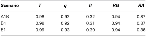
Table 2. Linear Pearson correlation coefficient for A1B, B1, and E1 scenarios for the period 2061–2090 for temperature, specific humidity, wind speed, surface solar radiation, and downward long-wave radiation.

Discussion

When dynamical downscaling is needed in impact or adaptation studies high temporal frequency atmospheric fields are required to force SVAT models. Future climate projections databases currently available for the whole Europe area have often daily frequency and for a grid point they provide only the daily mean or at the best the maximum and minimum values of atmospheric fields. This study presents a method to increase the temporal frequency of these variables from daily to hourly time step based on past near surface observations from a typical operational surface station. A statistical k-means method is applied to a construction period to classify observations in function of the type of the diurnal cycle for each variable. These clusters are identified in the future projections of climate and reconstructed sequences at hourly frequency are obtained.

Two sites in France were selected for this analysis, the Chartres station close to Paris (North-West of France) and Blagnac station close to Toulouse (South-West of France). The construction period was 1998–2008, the choice is based on the availability of hourly observations. Nine and eleven clusters were respectively identified for Paris and Toulouse. This number of clusters are considered enough to describe the climate variability in term of wind regimes, precipitation and thermal and humidity amplitude for both sites. Seasonal intra-cluster differences in the mean hourly cycles and differences in the circulations at the synoptic scale are also well represented.

Hourly reconstruction of 1961–1990 fields are compared to observations by means of the temporal evolution for a random period of 10 consecutive days for winter-time and summer-time, the scatter-plot and the linear Pearson correlation coefficient. The reconstruction algorithm is able to produce diurnal cycles that fits well with observations. The diurnal amplitude and mean value is well represented for variables with marked daily cycle as temperature or humidity. Changes in the mean wind direction are represented and, to a certain extent, changes in wind intensity are also retained. The mean precipitation is conserved during the day even if the method is not able to reproduce the short rain picks variability. Precipitation is used as input in the clusterization process and in clusters representative of rainy day some variability is in to a certain extent retained.

Finally, near-surface atmospheric outputs from Regional Climate Models have been reconstructed. Three runs from the MPI-REMO model at hourly frequency have been used to show the feasibility of the method for future projections of climate and pointed out the impact of omitting precipitation in the attribution process.

Six model outputs from the EU-FP6 ENSEMBLES were also reconstructed during the project at hourly frequency from the daily database. The ENSEMBLES database is a good example of a rich RCM scenarios database that are difficult to be exploited in the framework of off-line SVAT simulations for impact studies due to its temporal resolution. During the ENSEMBLES project climate groups from different countries performed ensemble simulations for Europe at 25 × 25 km² horizontal resolution for the A1B emission scenario. Seven model outputs were retained: ECHAM5-r3–RCA, ECHAM5-r3–RACMO, ECHAM5-r3–REMO; HadCM3Q0–CLM, HadCM3Q0–HadRM3Q0; BCM–RCA and BCM-DMI–HIRHAM5 (first name correspond to the forcing Global Climate model, the second name to the Regional Climate model). This choice was done in function of the availability of the following daily variables used in the attribution process (maximum, minimum and mean temperature and relative humidity, mean wind speed and direction, and mean precipitation) and period (at least runs from 1961 to 2090). Output time-series of daily modeled data are extracted at nearest grid point.

After a bias correction, a cluster number was attributed to every day of climate scenarios produced by these seven models using the method explained in Section First validation: cluster attribution and hourly reconstruction for the construction period (1998–2008).

From a statistical point of view mean values and climate variability are represented by Regional Climate Models but they do not reproduce the chronology of fields. For this reason, in absence of hourly scenarios, validation of reconstructed series from the ENSEMBLES database cannot be done with a day by day comparison as shown in Section Validation and Application to climate scenarios from Regional Climate Models simulations and only a statistical analysis makes sense. As modeled mean (and if available maximum and minimum) values are directly used, the hourly reconstructed series reproduce intensity of extreme events predicted by climate models and the temporal trends explored in typical climatic analysis as daily, seasonal or annual mean values. For impact studies where an accurate value of the length and intensity of extreme precipitation or gusts is needed, as for example in some hydrological or wind farms production impact studies, a complementary analysis of the clusters could be performed in order to obtain clusters where the precipitation or wind field has higher weight in the statistical analysis.

The main advantage of the method with regard to others cited in the introduction are the availability and light computing treatment of the data. The large coverage around the world of the meteorological stations makes the data collection easy and free available to anyone. The k-clustering algorithm is implemented in a variety of free programming languages and can be run in a simple computer or laptop. The attribution method is based on variables that are also available at daily frequency in climate scenarios databases so it is directly applicable to this kind of climate projections. Hourly reconstructed series are obtained using the observed (or modeled) mean value. If maximum and minimum values are also available, the shape of the cluster diurnal cycle is modulated in amplitude accordingly allowing extremes higher than those observed during the construction period if those are represented in the climate projections.

Even though interesting applications can be developed from the cluster attribution, for example to relate a kind of type of meteorological situation with impact factors in health as pollutants concentrations or thermal stress or to contextualize single field campaign days within a larger climatology. Also, with the aim of improve Regional Climate models parameterizations, it is possible to relate a type of day with strong biases in the RCM projections for a reference period to identify the physical process involved in this type of meteorological situations.

This method has been developed for local climate impact studies. In this case numerical simulations are performed over an area of some tenths of kilometers and, normally, only one site of observations is used to force the SVAT model at certain height over the canopy. It is during the numerical simulation that diagnostic atmospheric fields near the surface reproduces spatially the heterogeneity of the terrain. For bigger domains two types of strategies can be used to take into account observations (or model data) from a plurality of points. If the climatology of the area can be represented by a single set of clusters then one classification is done. In the attribution process, logically, the same type of day should be found for all sites and the reconstructed series for each site will reproduce the heterogeneity of observed (or simulated) fields. If in the attribution process there is no coherence between the sites, then, the domain should be divided into regions where the clustering method will be applied separately.

Conflict of Interest Statement

The authors declare that the research was conducted in the absence of any commercial or financial relationships that could be construed as a potential conflict of interest.

Acknowledgments

This research was performed at the GAME/CNRM (Météo-France, CNRS) supported by the French National Research Agency (ANR) under grant ANR-09-VILL-0003 and the Scientific Cooperation Foundation STAE in Toulouse in the context of the MUSCADE and the ACCLIMAT project respectively. Authors would like to thanks Nowlen Huet, Samuel Somot, and Michel Déqué from the CNRM for their constructive advice in the statistical and correction methods and Marien Lennart, Ralf Podzum, and Daniela Jacob, from the Climate Service Centre of the Max Planck Institute for Meteorology, that provided the hourly time-series from REMO simulations.

Supplementary Material

The Supplementary Material for this article can be found online at: http://www.frontiersin.org/journal/10.3389/fenvs.2014.00040/abstract

Footnotes

1. ^SVAT models simulate micro-scale energy and matter exchange processes between land surface and the atmospheric layer near the ground level. They are used by meteorologists, climatologists, ecologists, and biogeochemists to study the radiative transfer, the energy balance, the turbulent and diffusive transfer, the stomatal function, the photosynthesis and respiration, or the liquid phase water flow.

2. ^A previous bias correction should be performed using observed climate data in order to remove systematic errors from Global and Regional Climate models.

3. ^Similar results where obtained for repetition number of 5 and 30.

4. ^A fit function should be applied before long term simulations to avoid propagation of this signal to diagnosed fields.

References

Corti, S., Molteni, F., and Palmer, T. N. (1999). Signature of recent climate change in frequencies of natural atmospheric circulation regimes. Nature 398, 799–802. doi: 10.1038/19745

CrossRef Full Text | Google Scholar

Déqué, M., Martin, E., and Kitova, N. (2011). Response of the Snow Cover over France to Climate Change. Internal Communication. SCAMPEI project. Available online at: http://www.cnrm.meteo.fr/scampei/

Ducharne, A., Habets, F., Déqué, M., Evaux, L., Hachour, A., Lepaillier, et al. (2009). Impact du Changement Climatique sur les Ressources en eau et les Extrêmes Hydrologiques dans les Bassins de la Seine et la Somme, Rapport Final du Projet RExHySS, Programme GICC, 62. Available online at: http://www.sisyphe.jussieu.fr/~agnes/rexhyss/documents_rapport.php

Gonzalez-Aparicio, I., and Hidalgo, J. (2012). Dynamically based daily and seasonal future temperature scenarios analysis for the northern of Iberian Peninsula. Int. J. Climatol. 32, 1825–1833. doi: 10.1002/joc.2397

CrossRef Full Text | Google Scholar

He, J., Tan, A. H., Tan, C. L., and Sung, S. Y. (2002). “On quantitative evaluation of clustering systems,” in Information Retrieval and Clustering, eds W. Wu and H. Xiong (Kluwer Academic Publishers).

Google Scholar

Hewitt, C. D. (2005). The ENSEMBLES Project: providing ensemble-based predictions of climate changes and their impacts. EGGS newsletter. 13, 22–25. Available online at: http://www.the-eggs.org/?issueSel=24

Hidalgo, J. (2012a). Scénarios Climatiques Pour le Projet ACCLIMAT. Toulouse: Scientific report (in French).

Hidalgo, J. (2012b). Scénarios Climatiques Pour le Projet MUSCADE. Toulouse: Scientific report (in French).

Google Scholar

Huth, R., Beck, C., Philipp, A., Demuzere, M., Ustrnul, Z., Cahynová, M., et al. (2008). Classifications of atmospheric circulation patterns: recent advances and applications. Ann. N.Y. Acad. Sci. 1146, 105–152. doi: 10.1196/annals.1446.019

Pubmed Abstract | Pubmed Full Text | CrossRef Full Text | Google Scholar

Lemonsu, A., Kounkou-Arnaud, R., Desplat, J., Salagnac, J. L., and Masson, V. (2012). Evolution of the Parisian urban climate under a global changing climate. Clim. Change 116, 679–692. doi: 10.1007/s10584-012-0521-6

CrossRef Full Text | Google Scholar

Najac, J., Lac, C., and Terray, L. (2011). Impact of climate change on surface winds in France using a statistical-dynamical downscaling method with mesoscale modeling. Int. J. Climatol. 31, 415–430. doi: 10.1002/joc.2075

CrossRef Full Text | Google Scholar

Nakicenovic, N., Alcamo, J., Davis, G., de Vries, B., Fenhann, J., Gaffin, S., et al. (2000). IPCC Special Report on Emissions Scenarios. Cambridge: Cambridge University Press.

Philipp, A., Bartholy, J., Beck, C., Erpicum, M., Esteban, P., Fettweis, X., et al. (2010). Cost733cat - A database of weather and circulation type classifications. Phys. Chem. Earth 35, 360–373. doi: 10.1016/j.pce.2009.12.010

CrossRef Full Text | Google Scholar

Querguiner, S., Martin, E., Lafont, S., Calvet, J. C., Faroux, S., and Quintana-Seguí, P. (2012). Uncertainties associated to the representation of land surface processes in climate change impact studies: a case study for French Mediterranean regions. Nat. Hazards Earth Syst. Sci. 11, 2803–2816. doi: 10.5194/nhess-11-2803-2011

CrossRef Full Text

Quintana-Seguí, P., Ribes, A., Martin, E., Habets, F., and Boé, J. (2010). Comparison of three downscaling methods in simulating the impact of climate change on the hydrology of Mediterranean basins. J. Hydrol. 383, 111–124. doi: 10.1016/j.jhydrol.2009.09.050

CrossRef Full Text | Google Scholar

Quintana-Seguí, P., Habets, F., and Martin, E. (2011). Comparison of past and future Mediterranean high and low extremes of precipitation and river flow projected using different statistical downscaling methods. Nat. Hazards Earth Syst. Sci. 11, 1411–1432. doi: 10.5194/nhess-11-1411-2011

CrossRef Full Text | Google Scholar

Stone, D. A., Weaver, A. J., and Stouffer, R. J. (2001). Projection of climate change onto modes of atmospheric Variability. J. Clim. 14, 3551–3565. doi: 10.1175/1520-0442(2001)014%3C3551:POCCOM%3E2.0.CO;2

CrossRef Full Text | Google Scholar

Tanaka, K., Yoichi, F., Tsugihiro, W., Toshiharu, K., and Shuichi, I. (2006). Projection of the impact of climate change on the surface energy and water balance in the Seyhan River Basin Turkey. Annu. J. Hydraul. Eng. 50, 31–36. doi: 10.2208/prohe.50.31

CrossRef Full Text | Google Scholar