Current challenges in understanding and forecasting stable boundary layers over land and ice

Introduction

The atmospheric boundary layer over land experiences a clear diurnal cycle driven by that of the incoming solar radiation. During the evening transition period, the Earth's surface radiation budget turns negative due to longwave radiative loss and so the surface cools to a temperature below that of the air above. Consequently, the potential temperature increases with height, producing a stable boundary layer (SBL). SBLs prevail at night, but also during daytime in winter in mid-latitudes, in polar regions, and during daytime over irrigated regions with advection. The SBL is governed by a multiplicity of processes such as turbulence, radiative cooling, the interaction with the land surface, gravity waves, katabatic flows, fog and dew formation. Despite extensive earlier research, these processes and their interactions are not sufficiently understood, primarily because of their diversity and their general non-stationarity, which prevent an unambiguous interpretation of observations (Mahrt, 2007, 2014; Fernando and Weil, 2010). This ambiguity is a major obstacle to the development of model parameterizations. As a result, the SBL is inadequately represented in weather and climate models (e.g., Beljaars and Viterbo, 1998; Bechtold et al., 2008; Medeiros et al., 2011; Steeneveld et al., 2011; Kyselý and Plavcová, 2012; Tastula et al., 2012; Sterk et al., 2013; Bosveld et al., 2014). For instance, Atlaskin and Vihma (2012) studied the dependence of the 2-m temperature bias in multiple limited-area models on atmospheric stability for a winter period in Europe, and they found a warm bias in the 2-m temperature, increasing rapidly with stability.

Some models overestimate surface vegetation temperatures during calm nights (e.g., Steeneveld et al., 2008; Atlaskin and Vihma, 2012), while other models experience unrealistic decoupling of the atmosphere from the surface, resulting in so-called runaway surface cooling (e.g., Mahrt, 1998; Walsh et al., 2008). This contrasting behavior depends on differences in model formulation, resolution, and land-use properties. Furthermore, in order to obtain accurate forecasts of the synoptic flow, atmospheric models generally require a larger turbulent drag at the surface and in the boundary layer than can be justified from field observations (e.g., Holtslag et al., 2013). Hence the model representation of turbulent transport is generally based on model performance rather than on a physical basis. Unfortunately, the enhanced drag results in an underestimation of the wind turning with height within the SBL (Svensson and Holtslag, 2009). The SBL depth is usually too high, and the low-level jet speed underestimated when compared to observations. Also, models appear to underestimate the near-surface temperature and wind-speed gradient, and their diurnal cycle (Edwards et al., 2011). Those issues occur typically under very stable conditions. Moreover, model results are very sensitive to parameter values in the turbulence and orographic drag schemes (e.g., Beljaars et al., 2004; Sandu et al., 2013), which implies that it is challenging to achieve a high model skill for a wide range of states of the atmosphere-soil-vegetation system, and that compensating errors make it difficult to identify deficiencies in individual schemes. For these reasons, an enhanced understanding of the SBL and a more physical representation of the SBL in models is required. The overall aim of this mini-review is to present briefly the state-of-the-art, highlight the recent research activities on physical processes that received only limited attention so far, and to build a picture of the key processes and their interactions.

This review is organized as follows. Section Societal Impact summarizes the societal relevance of SBL processes. Section Physical Processes provides an overview of the physical processes acting in the SBL, their role, their interconnections and relevance for different SBL regimes. Section Role of SBL in Climate Debate briefly addresses the role of the SBL in understanding climate change. Finally, conclusions are drawn in Section Conclusion.

Societal Impact

The SBL is relevant to numerous applications in society. For instance, correct forecasting of near-surface temperatures and wind speed may improve road de-icing, as well as timely warnings to the transportation sector for low visibility caused by nocturnal fog or haze (van der Velde et al., 2010; Cuxart and Jiménez, 2011; Bartok et al., 2012). Agriculture relies on accurate near-surface frost forecasts to take measures to protect plants and yields (Prabha et al., 2011). Air quality forecasts and CO₂ inverse modeling studies call for reliable estimates of boundary-layer depth, wind speed, drainage flows, and turbulence intensity (Salmond and McKendry, 2005; Gerbig et al., 2008; Tolk et al., 2009). The wind energy sector requires hourly estimates of wind energy production, and thus relies on wind speed forecasts, particularly around hub height at 100 m above ground level (Storm and Basu, 2010).

In addition, Bony et al. (2006) found that the polar regions, which are generally stably stratified, are foreseen to warm 1.4–4 times faster than the global average in the period 1990–2090, but a clear reason for this is unknown. Recently, Pithan and Mauritsen (2014) evaluated the relative roles of the possible feedbacks responsible for this amplification. Surprisingly, the ensemble of the “Coupled Model Intercomparison Project-Phase 5” climate models indicates that it is not the ice-albedo-feedback that dominates, but temperature variations related to the surface energy balance and the vertical temperature structure provide the largest contribution to the amplification.

Physical Processes

The complexity of the SBL originates partly from the multiplicity of the processes involved. This section summarizes the main processes, their current state of knowledge, and associated open issues.

Turbulence

The nature of the atmospheric flow is characteristically turbulent, in which eddies of different scales absorb energy from the mean flow. These eddies break up into smaller eddies until they dissipate because of the action of molecular viscosity. All eddy motions of different length scales, from millimeters to the scale of the boundary-layer height (of order 100 m for the SBL), transport momentum, heat, humidity and contaminants. The turbulence intensity is influenced by wind shear and buoyancy. During daytime, the solar insolation heats the surface, and creates thermal instability and thermals, i.e., buoyancy dominates the turbulent kinetic energy budget. In contrast, in the SBL turbulence is suppressed by buoyancy during calm nights, and is produced only by wind shear. The net result is a precarious balance that is extremely sensitive to changes in the wind profile and the mean temperature profile.

Several turbulence regimes have been proposed. Although they differ in formulations (in terms of governing variables and threshold values), they all roughly distinguish between a so- called “weakly stable boundary layer” (WSBL), for which turbulence is the dominant transport process, and the “very stable boundary layer” (VSBL), for which turbulence is relatively weak. Within the WSBL, Nieuwstadt (1984) showed that scaling of local fluxes with the local gradients of wind and potential temperature works satisfactorily. Within the VSBL, a well-established scaling of turbulence variables and thermodynamic profiles is missing (e.g., van de Wiel et al., 2012). Qualitatively, this regime is determined by waves, drainage flows, weak turbulence and other (sub-)mesoscale motions, which are not necessarily of local nature. Recently, Mahrt et al. (2012) pointed out that for near-calm nocturnal conditions, significant turbulence is mainly generated by short-term (minutes-long) accelerations of unknown origin. Moreover, observations in the VBSL identified global and local intermittency of turbulence, but a conclusive framework for this phenomenon is still lacking (e.g., Nappo, 1991; van de Wiel et al., 2003; Costa et al., 2011).

Radiation

The radiation budget of the SBL addresses two aspects, i.e., the net radiation balance at the surface (Q*), and radiation divergence within the atmosphere. Q* is governed by the down- and upwelling longwave radiative fluxes. The first is largely determined from the atmospheric temperature and humidity profiles, and the latter is dominated by the surface temperature. Internal variability of these quantities may induce high-frequency harmonics of Q* within the SBL. Moreover, cloud cover variations and the evening transition trigger rapid Q* changes, which are usually challenging to represent in models (van de Wiel et al., 2003).

The energy transport by atmospheric radiation depends on the capacity to absorb and radiate energy to and from different atmospheric layers. This capacity is governed by the temperature of the layers, and the concentration of gases that are sensitive to interaction with radiation in the relevant range of wavelengths (e.g., water vapor, carbon dioxide, methane). Vertical radiation divergence is greater for larger vertical variations of temperature and especially humidity. Since these variations are large close to the surface, in particular for calm conditions, one may expect substantial radiation divergence near the surface. Indeed, numerous modeling studies reported such a divergence (Ha and Mahrt, 2003; Savijärvi, 2013). Field observations by Hoch et al. (2007) and Steeneveld et al. (2010) (Figure 1) reported radiation divergence values of several K/h in favorable conditions, particularly during sunset. Numerical models were found to underestimate substantially the radiative cooling for the case shown in Figure 1. Future research should clarify whether this model bias is a result from poor input to the radiation scheme, from the relatively coarse model resolution, or from deficiencies in the formulation of the radiation scheme (Wild et al., 2001; Rinke et al., 2012).

FIGURE 1

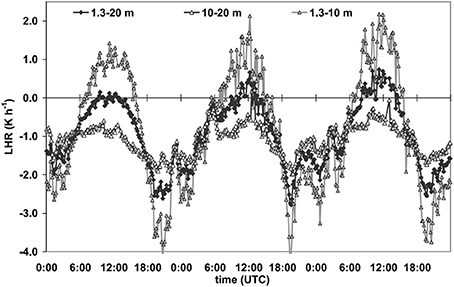
Figure 1. Observed longwave heating rate in three atmospheric layers for a series of clear calm days in May 2006, Wageningen, The Netherlands.

Orographically Induced Waves

Stratified flows allow for the propagation of gravity waves, generated for instance by hills and surface roughness transitions. Here, we limit ourselves to orographically induced waves, whose role in the SBL dynamics remains unclear (e.g., Brown et al., 2003). Since NWP models require more drag than is explained by turbulence observations, alternative processes that provide drag are worth to examine. Gravity waves generate drag, which might influence the dynamical evolution of the SBL. This mechanism is well understood for large mountain ridges. However, the SBL is shallow, and one can expect that small-scale orography can also significantly influence the SBL flow through gravity wave propagation. Using linear theory, Nappo (2002) indeed showed theoretically that the magnitude of the wave drag and turbulent drag can be of the same order for weak wind conditions.

Considering the complexity of real terrain, i.e., irregular hills, an alternative approach to estimate wave drag for these conditions is required. Figure S1 shows the estimated gravity wave drag (GWD) for four contrasting nights during the “Cooperative Atmospheric Surface Exchange Study 1999” (Steeneveld et al., 2009). During all nights the estimated GWD is of the same order of magnitude as the measured turbulent drag. During one night (9/10 Oct) the GWD is substantially larger than the turbulent drag for most of the night. In addition, the GWD is highly variable throughout the night, and varies on a timescale that is close to that of the observed global intermittent turbulence. Overall, these results suggest that orographically induced GWD is a possible candidate to explain in fact that drag is too small in NWP models.

The relevance of GWD is further illustrated by Burgering (2014) who studied the sensitivity of a numerical model to the application of GWD in the SBL on the large-scale flow development. That study evaluated the model score for sea-level pressure for an 8-day forecast over the Atlantic Ocean and Europe. When a relatively simple approach to account for GWD is implemented (Steeneveld et al., 2008; Lapworth, 2014), the root-mean- square error reduces by ~4 hPa (~40%) over a large portion of Europe for the studied cyclone. Also, the bias in the modeled cyclone core pressure was reduced by ~66%. Clearly, accounting for GWD in the SBL substantially improves the model accuracy compared to a run without this GWD.

Katabatic Winds

In general, the Earth's surface orography is relatively complex. Katabatic flows are ubiquitous features of SBLs on sloping surfaces that are cooled by a radiation deficit, for example over glaciers. In some areas, katabatic flows can govern the local climate substantially. Katabatic flows are characterized by a pronounced low-level jet and large near- surface temperature gradient. Hence katabatic flows affect the surface fluxes of heat, moisture and momentum, and consequently the ice mass budget over glaciers, but also over Greenland and the polar regions. The simplest model of katabatic flow represents a balance between negative buoyancy due to the surface potential temperature deficit, as the driving force, and turbulent drag that dampens the flow. On relatively long glaciers and at high latitudes, the Coriolis effect also influences katabatic flows, and induces a cross-slope wind component (Stiperski et al., 2007). This cross-slope wind is balanced by the Coriolis force and turbulent drag. Its vertical scale is larger than the characteristic height of the low-level jet of the down-slope component. The representation of katabatic flows in numerical weather prediction models is a challenging task (Grisogono et al., 2007; Jeričević et al., 2010).

Coupling to the Surface

Considering the fact that turbulent fluxes may vanish in the surface energy budget in calm conditions, the net radiation must then balance the ground heat flux in order to conserve the surface energy. Hence, it is evident that the land-surface coupling is important and should be accurately represented in atmospheric models, and its complexity should match the model complexity of parameterizations for other processes. Since the coupling with the land surface is an integral part of the SBL physics, studies using prescribed temperature, particularly with prescribed fluxes should be avoided. This aspect is further discussed in Holtslag et al. (2007), who showed within a model intercomparison context that model output variability is strongly reduced when the atmospheric model is coupled to the land surface instead of prescribing the surface temperature.

Weather and climate models require numerical values for the heat conductivity, which are highly uncertain at the grid scale, especially for snow-covered surfaces. Dutra et al. (2012) quantified the EC-EARTH model performance and concluded that a correct thermal insulation of the snowpack is essential to improve the realism of the near-surface atmospheric temperature. Moreover, their multilayer snow scheme outperforms the single-layer scheme in deep snowpacks. Furthermore, an increased snow thermal insulation removed a warm bias over snow-covered regions during winter and spring; Cook et al. (2008) reported an analogous sensitivity in which high vs. low insulation led to soil cooling of up to 20 K in winter and 2-m temperature warming of 6 K.

Interactions

Figure 2 summarizes the mentioned processes and their interactions; herein positive (negative) feedbacks indicate a strengthening (weakening) of the process at the end of the arrow. First we identify the pressure-gradient force, the Coriolis force, cloud cover, free-flow stability, and deep-soil temperature as external driving variables. Low cloud cover strengthens the net radiative surface cooling, and thereby reduces the surface temperature and builds up the stratification. While stratification builds up, it slowly erodes by radiation divergence which acts to overcome the temperature contrast. On the other hand, an increased pressure gradient raises the wind speed, and consequently the turbulent mixing. A stronger mixing erodes the thermal stratification, resulting in a smaller magnitude of the sensible heat flux in the WSBL. Stronger mixing tends to deepen the SBL against the free flow stability and Coriolis parameter. However, a contrasting direction is found in the VSBL, where a reduced stratification might result in an increased sensible heat flux. In both cases the other surface energy budget components (soil heat flux and dew) and the surface vegetation temperature will be modified. The altered surface temperature establishes a new stratification, which consequently feedbacks to the surface radiation balance.

FIGURE 2

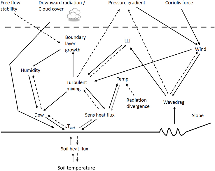
Figure 2. Schematic overview of physical processes in the stable boundary layer over land, including their interactions and positive (——) and negative feedbacks (-----). Gray lines indicate processes that can have either a positive or negative feedback, depending on the state of the boundary layer.

Another feedback loop evolves via the proportionality between GWD and wind speed, thereby strengthening the cyclone filling rate, and thus reducing the pressure gradient and geostrophic wind. Near the surface, GWD enhances the low-level jet wind speed, providing additional downward turbulent mixing from the jet, and thereby moderating the stratification again. In case of sloping terrain, cold air pooling triggers pronounced local temperature effects. Hence the SBL evolution is driven by a complex interplay between a myriad of processes, which presents a challenge for an accurate representation of the SBL in models.

Role of SBL in Climate Debate

The ongoing climate change is mostly observed at night and under stable conditions (Vose et al., 2005). The vertical distribution of added heat is essential to an interpretation of the 2-m temperature. Recently, Steeneveld et al. (2011) and McNider et al. (2012) performed a single-column model experiment in which the impact of enhanced CO₂ concentration on the 2-m temperature was quantified for a wide range of geostrophic wind speeds. They found that feedbacks in the SBL and the land surface provide a 2-m temperature rise that is rather constant over a relatively broad range of geostrophic wind speeds. Apparently, the enhanced longwave downward radiation at the surface alters the surface temperature, reducing the surface stability, which consequently enhances the mixing in the whole SBL. Hence, vertical redistribution of heat through the SBL may amplify or dampen the 2-m temperature signal. This means that the 2-m temperature as a climate diagnostic needs to be re-evaluated. As a contribution to this discussion, Esau et al. (2012) hypothesized that the spatiotemporal variability of climate change is partly related to the effective heat capacity of the atmosphere, i.e., it is related to the boundary-layer depth. They showed that the largest temperature changes occur in areas with a relatively shallow boundary-layer depth.

Conclusion

The SBL is governed by a myriad of physical processes. The weakly-stable boundary layer is dominated by well-developed turbulence that follows local scaling, and this regime can be relatively well modeled and forecast. Within the very stable regime, processes such as radiation divergence, orographic drag, land-surface coupling and (sub-)mesoscale motions can play a major role in the evolution of the SBL. These processes have not yet been fully understood and their relative impact has not yet been quantified. To advance our knowledge of the SBL it is essential that atmospheric models represent these processes as purely as possible. In terms of model development, this means that a strict splitting of the processes should be preferred over the current approach that lumps the net effect of many small-scale processes within a single parameterization scheme, e.g., a stability function in the boundary-layer scheme. This preferred approach will open the way for a better understanding of the SBL and an improved representation of it in NWP and climate models.

Conflict of Interest Statement

The author declares that the research was conducted in the absence of any commercial or financial relationships that could be construed as a potential conflict of interest.

Acknowledgments

The author acknowledges NWO VENI grant “Lifting the fog” (contract number 863.10.010), and all co-workers who contributed to this mini-review, i.e., Bert Holtslag, Liduin Burgering, Michal Kleczek, Marina Sterk, Bert Heusinkveld, Christine Groot Zwaaftink, Marcel Wokke, Sander Pijlman (Wageningen University), Bas van de Wiel (TU Eindhoven), Richard Bintanja (Royal Netherlands Meteorological Institute), Carmen Nappo (CJN Research Meteorology).

Supplementary Material

The Supplementary Material for this article can be found online at: http://www.frontiersin.org/journal/10.3389/fenvs.2014.00041/abstract

Figure S1 | Modeled surface wave stress components (lines), and measured turbulent stress (+) for a series of nights during the Cooperative Atmospheric Surface Exchange Study 1999. In the header the classification of van de Wiel et al. (2003) (Turb, Rad, Non) is indicated. (U_g, V_g) identify the geostrophic wind for the simulation.

References

Atlaskin, E., and Vihma, T. (2012). Evaluation of NWP results for wintertime nocturnal boundary-layer temperatures over Europe and Finland. Q. J. R. Meteorol. Soc. 138, 1440–1451. doi: 10.1002/qj.1885

CrossRef Full Text | Google Scholar

Bartok, J., Bott, A., and Gera, M. (2012). Fog prediction for road traffic safety in a coastal desert region. Bound. Lay. Meteorol. 145, 485–506. doi: 10.1007/s10546-012-9750-5

CrossRef Full Text

Bechtold, P., Köhler, M., Jung, T., Doblas-Reys, F., Letbecher, M., Rodwell, M. J., et al. (2008). Advances in simulating atmospheric variability with the ECMWF model: from synoptic to decadal time-scales. Q. J. R. Meteorol. Soc. 134, 1337–1351. doi: 10.1002/qj.289

CrossRef Full Text | Google Scholar

Beljaars, A. C. M., Brown, A. R., and Wood, N. (2004). A new parameterization of turbulent orographic form drag. Q. J. R. Meteorol. Soc. 130, 1327–1347. doi: 10.1256/qj.03.73

CrossRef Full Text | Google Scholar

Beljaars, A. C. M., and Viterbo, P. (1998). “Role of the boundary layer in a numerical weather prediction model,” in Clear and Cloudy Boundary Layers, eds A. A. M. Holtslag, and P. G. Duynkerke (Amsterdam: Royal Netherlands Academy of Arts and Sciences), 372.

Google Scholar

Bony, S., Colman, R., Kattsov, V. M., Allan, R. P., Bretherton, C. S., Dufresne, J.-L., et al. (2006). How well do we understand and evaluate climate change feedback processes? J. Clim. 19, 3445–3482. doi: 10.1175/JCLI3819.1

Pubmed Abstract | Pubmed Full Text | CrossRef Full Text | Google Scholar

Bosveld, F. C., Baas, P., Steeneveld, G. J., Holtslag, A. A. M., Angevine, W. M., Bazile, E., et al. (2014). The GABLS third intercomparison case for model evaluation, Part B: SCM model intercomparison and evaluation, Bound. Lay. Meteorol. 152, 157–187. doi: 10.1007/s10546-014-9919-1

CrossRef Full Text

Brown, A. R., Athanassiadou, M., and Wood, N. (2003). Topographically induced waves within the stable boundary layer. Q. J. R. Meteorol. Soc. 129, 3357–3370. doi: 10.1256/qj.02.176

CrossRef Full Text | Google Scholar

Burgering, L. M. T. (2014). Modeling Orographic Gravity Wave Drag in the Stable Boundary Layer and Determining the Influence on Cyclonic Filling. MSc thesis report, Wageningen University, Wageningen, 68.

Cook, B. I., Bonan, G. B., Levis, S., and Epstein, H. E. (2008). The thermoinsulation effect of snow cover within a climate model. Clim. Dyn. 31, 107–124. doi: 10.1007/s00382-007-0341-y

CrossRef Full Text | Google Scholar

Costa, F. D., Acevedo, O. C., Mombach, J. C. M., and Degrazia, G. A. (2011). A simplified model for intermittent turbulence in the nocturnal boundary layer. J. Atmos. Sci. 68, 1714–1729. doi: 10.1175/2011JAS3655.1

CrossRef Full Text | Google Scholar

Cuxart, J., and Jiménez, M. A. (2011). Deep radiation fog in a wide closed valley: study by numerical modeling and remote sensing. Pure Appl. Geophys. 169, 911–926. doi: 10.1007/s00024-011-0365-4

CrossRef Full Text | Google Scholar

Dutra, E., Viterbo, P., Miranda, P. M. A., and Balsamo, G. (2012). Complexity of snow schemes in a climate model and its impact on surface energy and hydrology. J. Hydrometeorol. 13, 521–538. doi: 10.1175/JHM-D-11-072.1

CrossRef Full Text | Google Scholar

Edwards, J. M., McGregor, J. R., Bush, M. R., and Bornemann, F. J. A. (2011). Assessment of numerical weather forecasts against observations from Cardington: seasonal diurnal cycles of screen-level and surface temperatures and surface fluxes. Q. J. R. Meteorol. Soc. 137, 656–672. doi: 10.1002/qj.742

CrossRef Full Text | Google Scholar

Esau, I., Davy, R., and Outten, S. (2012). Complementary explanation of temperature response in the lower atmosphere. Environ. Res. Lett. 7:044026. doi: 10.1088/1748-9326/7/4/044026

CrossRef Full Text | Google Scholar

Fernando, H. J. S., and Weil, J. C. (2010). Whither the stable boundary layer? A shift in the research agenda. Bull. Am. Meteorol. Soc. 91, 1475–1484. doi: 10.1175/2010BAMS2770.1

CrossRef Full Text | Google Scholar

Gerbig, C., Körner, S., and Lin, J. C. (2008). Vertical mixing in atmospheric tracer transport models: error characterization and propagation. Atmos. Chem. Phys. 8, 591–602. doi: 10.5194/acp-8-591-2008

CrossRef Full Text | Google Scholar

Grisogono, B., Kraljević, L., and Jeričević, A. (2007). The low-level katabatic jet height versus Monin-Obukhov height. Q. J. R. Meteorol. Soc. 133, 2133–2136. doi: 10.1002/qj.190

CrossRef Full Text | Google Scholar

Ha, K. J., and Mahrt, L. (2003). Radiative and turbulent fluxes in the nocturnal boundary layer. Tellus 55A, 317–327. doi: 10.1034/j.1600-0870.2003.00031.x

CrossRef Full Text | Google Scholar

Hoch, S. W., Calanca, P., Philipona, R., and Ohmura, A. (2007). Year-Round observation of longwave radiative flux divergence in Greenland. J. Appl. Meteorol. Clim. 45, 1469–1479. doi: 10.1175/JAM2542.1

CrossRef Full Text | Google Scholar

Holtslag, A. A. M., Steeneveld, G. J., and van de Wiel, B. J. H. (2007). Role of land-surface feedback on model performance for the stable boundary layer. Bound. Lay. Meteorol. 125, 361–376. doi: 10.1007/978-0-387-74321-9_14

CrossRef Full Text | Google Scholar

Holtslag, A. A. M., Svensson, G., Baas, P., Basu, S., Beare, B., Beljaars, A. C. M., et al. (2013). Stable atmospheric boundary layers and diurnal cycles: challenges for weather and climate models. Bull. Am. Meteorol. Soc. 94, 1691–1706. doi: 10.1175/BAMS-D-11-00187.1

CrossRef Full Text | Google Scholar

Jeričević, A., Kraljević, L., Grisogono, B., Fagerli, H., and Večenaj, Ž. (2010). Parameterization of vertical diffusion and the atmospheric boundary layer height determination in the EMEP model. Atmos. Chem. Phys. 10, 341–364. doi: 10.5194/acp-10-341-2010

CrossRef Full Text | Google Scholar

Kyselý, J., and Plavcová, E. (2012). Biases in the diurnal temperature range in Central Europe in an ensemble of regional climate models and their possible causes. Clim. Dyn. 39, 1275–1286. doi: 10.1007/s00382-011-1200-4

CrossRef Full Text | Google Scholar

Lapworth, A. (2014). Observations of the site dependency of the morning wind and the role of gravity waves in the transitions. Q. J. R. Meteorol. Soc. doi: 10.1002/qj.2340. [Epub ahead of print].

CrossRef Full Text | Google Scholar

Mahrt, L. (1998). Stratified atmospheric boundary layers and breakdown of models. Theor. Comput. Fluid Phys. 11, 263–279. doi: 10.1007/s001620050093

CrossRef Full Text | Google Scholar

Mahrt, L. (2007). Weak-wind mesoscale meandering in the nocturnal boundary layer. Environ. Fluid Mech. 7, 331–347. doi: 10.1007/s10652-007-9024-9

CrossRef Full Text | Google Scholar

Mahrt, L. (2014). Stably stratified atmospheric boundary layers. Annu. Rev. Fluid Mech. 46, 23–45. doi: 10.1146/annurev-fluid-010313-141354

Pubmed Abstract | Pubmed Full Text | CrossRef Full Text | Google Scholar

Mahrt, L., Richardson, S., Seaman, N., and Stauffer, D. (2012). Turbulence in the nocturnal boundary layer with light and variable winds. Q. J. R. Meteorol. Soc. 138, 1430–1439. doi: 10.1002/qj.1884

CrossRef Full Text | Google Scholar

McNider, R. T., Steeneveld, G. J., Holtslag, A. A. M., Pielke, R. A. Sr., Mackaro, S., Pour-Biazar, A., et al. (2012). Response and sensitivity of the nocturnal boundary layer to added longwave radiative forcing. J. Geophys. Res. 117:D14106. doi: 10.1029/2012JD017578

CrossRef Full Text | Google Scholar

Medeiros, B., Deser, C., Tomas, R. A., and Kay, J. E. (2011). Arctic inversion strength in climate models. J. Clim. 24, 4733–4740. doi: 10.1175/2011JCLI3968.1

CrossRef Full Text | Google Scholar

Nappo, C. J. (1991). Sporadic breakdowns of stability in the PBL over simple and complex terrain. Bound. Lay. Meteorol. 54, 69–87. doi: 10.1007/BF00119413

CrossRef Full Text | Google Scholar

Nappo, C. J. (2002). An Introduction to Atmospheric Gravity Waves. London: Academic Press.

Google Scholar

Nieuwstadt, F. T. M. (1984). The turbulent structure of the stable, nocturnal boundary layer. J. Atmos. Sci. 41, 2202–2216. doi: 10.1175/1520-0469(1984)041<2202:TTSOTS>2.0.CO;2

CrossRef Full Text | Google Scholar

Pithan, F., and Mauritsen, T. (2014). Arctic amplification dominated by temperature feedbacks in contemporary climate models. Nat. Geosci. 7, 181–184. doi: 10.1038/ngeo2071

CrossRef Full Text | Google Scholar

Prabha, T. V., Hoogenboom, G., and Smirnova, T. G. (2011). Role of land surface parameterizations on modeling cold-pooling events and low-level jets. Atmos. Res. 99, 147–161. doi: 10.1016/j.atmosres.2010.09.017

CrossRef Full Text | Google Scholar

Rinke, A., Ma, Y., Bian, L., Xin, Y., Dethloff, K., Persson, P. O. G., et al. (2012). Evaluation of atmospheric boundary layer–surface process relationships in a regional climate model along an East Antarctic traverse. J. Geophys. Res. 117:D09121. doi: 10.1029/2011JD016441

CrossRef Full Text | Google Scholar

Salmond, J. A., and McKendry, I. G. (2005). A review of turbulence in the very stable boundary layer and its implications for air quality. Prog. Phys. Geogr. 29, 171–188. doi: 10.1191/0309133305pp442ra

CrossRef Full Text | Google Scholar

Sandu, I., Beljaars, A., Bechtold, P., Mauritsen, T., and Balsamo, G. (2013). Why is it so difficult to represent stably stratified conditions in numerical weather prediction (NWP) models? J. Adv. Modell. Earth Syst. 5, 117–133. doi: 10.1002/jame.20013

CrossRef Full Text | Google Scholar

Savijärvi, H. (2013). High-resolution simulations of the night-time stable boundary layer over snow. Q. J. R. Meteorol. Soc. 140, 1121–1128. doi: 10.1002/qj.2187

CrossRef Full Text | Google Scholar

Steeneveld, G. J., Holtslag, A. A. M., McNider, R. T., and Pielke, R. A. (2011). Screen level temperature increase due to higher atmospheric carbon dioxide in calm and windy nights revisited. J. Geophys. Res. 116:D02122. doi: 10.1029/2010JD014612

CrossRef Full Text | Google Scholar

Steeneveld, G. J., Holtslag, A. A. M., Nappo, C. J., van de Wiel, B. J. H., and Mahrt, L. (2008). Exploring the possible role of small-scale terrain drag on stable boundary layers over land. J. Appl. Meteorol. Climatol. 47, 2518–2530. doi: 10.1175/2008JAMC1816.1

CrossRef Full Text | Google Scholar

Steeneveld, G. J., Nappo, C. J., and Holtslag, A. A. M. (2009). Estimation of orographically induced wave drag in the stable boundary layer during CASES99. Acta Geophys. 57, 857–881. doi: 10.2478/s11600-009-0028-3

CrossRef Full Text | Google Scholar

Steeneveld, G. J., Wokke, M. J. J., Groot Zwaaftink, C. D., Pijlman, S., Heusinkveld, B. G., Jacobs, A. F. G., et al. (2010). Observations of the radiation divergence in the surface layer and its implication for its parametrization in numerical weather prediction models. J. Geophys. Res. 115:D06107. doi: 10.1029/2009JD013074

CrossRef Full Text | Google Scholar

Sterk, H. A. M., Steeneveld, G. J., and Holtslag, A. A. M. (2013). The role of snow-surface coupling, radiation, and turbulent mixing in modeling a stable boundary layer over Arctic sea ice. J. Geophys. Res. Atmos. 118, 1199–1217. doi: 10.1002/jgrd.50158

CrossRef Full Text | Google Scholar

Stiperski, I., Kavčič, I., Grisogono, B., and Durran, D. R. (2007). Including coriolis effects in the prandtl model for katabatic flow. Q. J. R. Meteorol. Soc. 133, 101–106. doi: 10.1002/qj.19

CrossRef Full Text | Google Scholar

Storm, B., and Basu, S. (2010). The WRF model forecast-derived low-level wind shear climatology over the United States Great Plains. Energies 3, 258–276. doi: 10.3390/en3020258

CrossRef Full Text | Google Scholar

Svensson, G., and Holtslag, A. A. M. (2009). Analysis of model results for the turning of the wind and related momentum fluxes in the stable boundary layer. Bound. Lay. Meteorol. 132, 261–277. doi: 10.1007/s10546-009-9395-1

CrossRef Full Text | Google Scholar

Tastula, E.-M., Vihma, T., and Andreas, E. L. (2012). Evaluation of Polar WRF from modeling the atmospheric boundary layer over antarctic sea ice in autumn and winter. Mon. Wea. Rev. 140, 3919–3935. doi: 10.1175/MWR-D-12-00016.1

CrossRef Full Text | Google Scholar

Tolk, L. F., Peters, W., Meesters, A. G. C. A., Groenendijk, M., Vermeulen, A. T., Steeneveld, G. J., et al. (2009). Modelling regional scale surface fluxes, meteorology and CO2 mixing ratios for the Cabauw tower in the Netherlands. Biogeosciences 6, 2265–2280. doi: 10.5194/bg-6-2265-2009

CrossRef Full Text | Google Scholar

van de Wiel, B. J. H., Moene, A. F., Hartogensis, O. K., De Bruin, H. A. R., and Holtslag, A. A. M. (2003). Intermittent turbulence and oscillations in the stable boundary-layer over land. Part III: a classification for observations during CASES99. J. Atmos. Sci. 60, 2509–2522. doi: 10.1175/1520-0469(2003)060<2509:ITITSB>2.0.CO;2

CrossRef Full Text | Google Scholar

van de Wiel, B. J. H., Moene, A. F., Jonker, H. J. J., Baas, P., Basu, S., Donda, J. M. M., et al. (2012). The minimum wind speed for sustainable turbulence in the nocturnal boundary layer. J. Atmos. Sci. 69, 3116–3127. doi: 10.1175/JAS-D-12-0107.1

CrossRef Full Text | Google Scholar

van der Velde, I. R., Steeneveld, G. J., Wichers Schreur, B. G. J., and Holtslag, A. A. M. (2010). Modeling and forecasting the onset and duration of severe radiation fog under frost conditions. Mon. Wea. Rev. 138, 4237–4253. doi: 10.1175/2010MWR3427.1

CrossRef Full Text | Google Scholar

Vose, R. S., Easterling, D. R., and Gleason, B. (2005). Maximum and minimum temperature trends for the globe: an update through 2004. Geophys. Res. Lett. 32:L23822. doi: 10.1029/2005GL024379

CrossRef Full Text | Google Scholar

Walsh, J. E., Chapman, W. L., Romanovsky, V., Christensen, J. H., and Stendel, M. (2008). Global climate model performance over Alaska and Greenland. J. Clim. 21, 6156–6174. doi: 10.1175/2008JCLI2163.1

CrossRef Full Text | Google Scholar

Wild, M., Ohmura, A., Gilgen, H., Morcrette, J. J., and Slingo, A. (2001). Evaluation of downward longwave radiation in general circulation models. J. Clim. 14, 3227–3239. doi: 10.1175/1520-0442(2001)014<3227:EODLRI>2.0.CO;2

CrossRef Full Text | Google Scholar