Studying geometric structures in meso-scale flows

Introduction

Geometric shapes of coherent structures such as ramp or cliff like signals, step changes and waves in meteorological temporal series, are commonly observed during atmospheric measurements. Scientific interest on coherent structures was intensified after a number of studies indicated that they might dominate the turbulent energy and mass exchange between the atmospheric surface layer and the layers above (e.g., Gao et al., 1989; Serafimovich et al., 2011). Also, from a theoretical point of view it was proposed recently that, under the presence of large organized structures, highly complex atmospheric turbulent flows start behaving as low dimensional chaotic systems (Wesson et al., 2003; Campanharo et al., 2008).

The existence of ramp like structures in turbulence is well established and measured in field and laboratory. It was Taylor that as early as 1958 described “assymetrical triangular waves of temperature (gradual rise followed by a sudden drop)” in the atmospheric boundary layer and he attributed their shape to the convective plumes (Taylor, 1958). Since then, numerous studies have reported geometrical shapes of coherent structures over a variety of surfaces such as land (e.g., Barthlott et al., 2007), ice (e.g., Lykossov and Wamser, 1995), vegetation (e.g., Serafimovich et al., 2011), and water (e.g., Boppe et al., 1999). Ramp-like coherent structures under unstable conditions have been attributed mainly to surface-layer plumes or mixed-layer thermals (e.g., Kaimal and Businger, 1970) but also superposition of shear driven and thermal structures has been reported (Thomas and Foken, 2006). Coherent structures were also detected in stable flows (Kikuchi and Chiba, 1985), and they might appear without the presence of a boundary (Belušić and Mahrt, 2012).

Structural shapes have also been detected in larger (temporal and spatial) scale flows. For example in the sub-meso region (scales just larger than the turbulence scale), step changes in temperature time series associated with micro-front passage have been detected (Mahrt, 2010), and wave-like motions such as solitary waves have been reported as evolving from density currents in the stable lower atmosphere (Koch et al., 2008). In the meso-scale region, the association of specific shapes with physical processes is not an easy task, since a melange of different modes are often experienced, such as micro-fronts, meandering motions, drainage flows, shear instabilities, gravity waves etc. (Belušić and Mahrt, 2012; Stull, 1988).

A variety of conditional sampling techniques have been developed in order to objectively identify structural shapes in meteorological time series, and often contradictory interpretations of results obtained with different methods are reported (Krusche and De Oliveira, 2004, and references therein). Recently, Belušić and Mahrt (2012) introduced a simple linear technique to extract geometrical shapes that are usually observed in small scale turbulence and in meso-scale flows. They applied the technique to temperature and wind speed time series measured at Kutina, Croatia, for different scales (from 3 s up to 2 h: thus covering a wide range of the turbulent and meso-scales). They found a minimum in the number of recognized structures at time scales between 2 and 10 min in accordance with the known minimum of kinetic energy between turbulence and mesoscales. They also proposed that the relationships between the basic geometrical shapes are independent of the scale under consideration, despite the changing physics.

Strictly speaking, coherent structures directly refer to large spatially organized motions; in that sense the use of several anemometers at different heights or horizontally close locations is required in order to explicitly reveal the coherent spatial structures. The inference of coherent structure characteristics from time traces obtained from a stationary sensor has been used (e.g., in Wesson et al., 2003) with the implicit assumption of Taylor's hypothesis of frozen turbulence, i.e., that the advection velocity of the eddy (turbulence) is much greater than the velocity scale of the turbulence itself. Even though application of Taylor's hypothesis might induce non-negligible errors in certain cases (Zaman and Hussain, 1981), it has been pointed out that large atmospheric structures tend to be long lived and therefore are the best candidates for the applicability of Taylor's hypothesis (Higgins et al., 2012). Here we apply the term “geometrical structures” for shapes detected in wind speed and temperature time series related with mesoscale atmospheric motions, such as sea breezes and down-slope winds.

In this work the same technique described above has been applied at a dataset which had been obtained at a location experiencing a number of different mesoscale modes (Kallos et al., 1993; Helmis et al., 1995; Helmis and Papadopoulos, 1996). The aim of this work is to extract the geometrical characteristics of the 1 h time scales and then to relate the extracted structures with aspects of the mesoscale flows.

Materials and Methods

Experimental Site

In this work, the Automatic Meteorological Station (AMS) of the Lab of Meteorology of the Physics Department, University of Athens which is located at the University Campus on the eastern foothills of Hymettus mountain, 5 km from the city center, was used. The experimental site as well as the instrumentation used are analytically described in Halios et al. (2012). For the present study we used a dataset of 1 min measurements of atmospheric pressure (P, hPa), temperature (T, C), relative humidity (RH, %), solar radiation (SR, W m⁻²), wind speed and direction (WS and WD, ms⁻¹, degrees respectively) measured at 10 m and wind shear between 10 and 5 m agl, for the time period 11/1/2000–23/5/2000.

Geometric Structures

In the following, the basic steps of the methodology employed for the identification of geometric structures are briefly described. Full details of the methodology can be found in Belušić and Mahrt (2012).

(a) Initially four basic geometric shapes were chosen:

• a ramp-cliff function (gradual rise in time series followed by a sudden drop),

• a cliff-ramp function (or a reversed ramp-cliff: sudden rise followed by a gradual drop),

• a step function, and

• a simple sine function.

Each shape can have two orientations: the shape can start with a positive or negative gradient (mathematically expressed as the parameter's time derivative- d/dt); thus we end up with eight shapes which are used for further analysis (see Figure 6 and also Figure 2 in Belušić and Mahrt, 2012). Consequently 8 time series each of 60 data points were created, each one corresponding to one of the eight pre-defined structures.

(b) Each geometric shape of 60 data points move step-by-step through the time series under consideration (wind speed and temperature) and for each location (consisting of 60 points) the correlation coefficient is calculated. Parts with 60 points (minutes) in the time series which have a correlation coefficient >0.9 with the pre-selected shape are selected and categorized under the specific structure; for the step and sine structures extra filters are applied, in order to avoid misinterpretation.

(c) The part of the time series that was just recognized as being part of the specific shape is deleted, and excluded from further analysis.

(d) The procedure for the specific shape is completed after all parts with r > 0.9 have been selected.

(e) The procedure begins for the next geometric shape.

Meso-Scale Flows

The characteristics of the meso-scale flows and general meteorological conditions were studied using two methodologies: (1) a Principal Component Analysis (PCA) for the determination of the dominant surface patterns which was previously applied to a wider dataset from the same location and (2) an analysis of the so-called Integral quantities which are used to characterize stagnation, recirculation and ventilation conditions (Allwine and Whiteman, 1994). The two methods are briefly discussed in the following.

Principal component analysis

With PCA a dataset, which contains a large number of variables is reduced to a new dataset containing fewer new variables (Principal Components). Principal Components are linear combinations of the original variables, which are chosen to represent the maximum possible fraction of the variability contained in the original data. Thus, subgroups of variables are defined, which co-vary similarly in time. During the last several decades this method has been extensively used in the various branches of atmospheric science (see for example Jollife, 2002). PCA was successfully employed to categorize the meso-scale flows in this particular location (Halios et al., 2012). The original data were transformed according to the Box and Cox method (Wilks, 2006).

Analysis of integral quantities

In Allwine and Whiteman (1994) a method was proposed for the objective measure of air mass stagnation, recirculation and ventilation, based on single station integral measures of wind data. The method runs as follows: considering a time series of I = 1 … n discrete observations of wind speed (V_i) and direction (WD_i) at a single measuring site, the north-south (positive toward north) and east-west (positive toward east) components would be resolved as:

$\begin{array}{l}{v}_i=U_i\cos (W{D}_i-180),\\ u_i=U_i\sin (W{D}_i-180)\end{array}$

Then at each time step t_i the following discrete integral quantities are defined:

- The “resultant transport distance” (L). This is the net vector displacement, ‘which is obtained from the north—south $X_i=T{\displaystyle \sum _{j=i}^{i-\tau /T+1}{v}_j}$ and east-west $Y_i=T{\displaystyle \sum _{j=i}^{i-\tau /T+1}{u}_j}$ transport distances, considering that $L_i=\sqrt{X_i^2+Y_i^2}$. Then it follows that $L_i=T\left|{\displaystyle \sum _{j=i}^{i-\tau /T+1}{V}_j}\right|=T{\left[{\left({\displaystyle \sum _{j=i}^{i-\tau /T+1}{u}_j}\right)}^2+{\left({\displaystyle \sum _{j=i}^{i-\tau /T+1}{v}_j}\right)}^2\right]}^{\frac{1}{2}}$.

- The “wind run” (S), which is the wind scalar sum and is calculated as $S_i=T{\displaystyle \sum _{j=i}^{i-\tau /T+1}\left|V_j\right|}=T{\displaystyle \sum _{j=i}^{i-\tau /T+1}{\left(u_j^2+v_j^2\right)}^{\frac{1}{2}}}$.

- The “recirculation factor” (R) which is based on the ratio between L and S: $R_i=1-\frac{S_i}{L_i}$.

T is the averaging interval in hours (say, 1 h) and τ is the wind run time for integration (e.g., 24 h). In the present study L, S, and R values are looking backward in time whereas in Allwine and Whiteman (1994) study are looking forward. There, critical values of S and R are proposed for the characterization of the flow: thus for S_i < 120 km the site is prone to stagnation, for R_i > 0.6 prone to recirculation, and for R_i < 0.2 and S_i > 250 km the site is prone to ventilation.

Results

Mesoscale Flows

Three PCs accounting for 77.4% of the total variance were rotated with varimax Rotation, and are interpreted according to the values of the respective loadings (Table 1). PC2 contrasts temperature and solar radiation to humidity (correlation coefficients 0.81, 0.72, and −0.76, respectively). The other two PCs (PC1 and PC3, respectively) are related with the along (v) and across (u) axis mountain components of the wind speed. PC1, (related to the along-mountain wind speed component, correlation coefficient 0.91) is also highly correlated with intense changes in the wind speed (R = 0.89) and wind shear (R = 0.83); thus it is related with mechanically generated turbulence. Finally PC3 is related mainly with the u-component of the wind speed (R = 0.96), and also moderately correlated with intense changes in the wind speed (R = 0.32) and shear (R = 0.33). These results were also found in Halios et al. (2012), the only different aspect being the wind direction standard deviation. In that study it was proposed that the PC which is related with the along the mountain axis wind component, was related with persistent flows, while the PC related with the across the mountain axis wind component was related with a weak and variable flow. It was found that a strong, steady wind flow characterized by high shear values develops under the cyclonic Closed Low and the anti-cyclonic H–L categories, in contrast to the variable weak flow which occurs mainly under the anti-cyclonic Open Anticyclone category.

TABLE 1

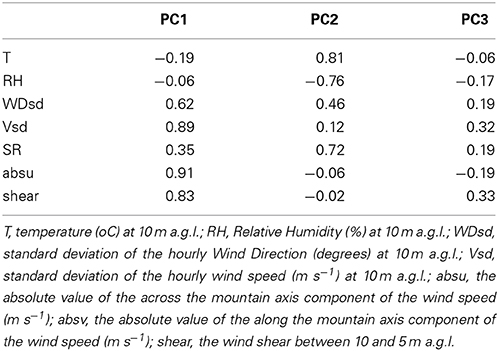
Table 1. PC loadings from principal component analysis.

In Figure 1 results from the analysis proposed by Allwine and Whiteman (1994) is shown. It can be seen that out of the 2294 cases, 25% were categorized as ventilation conditions, 7% as recirculation conditions and 3% as stagnant conditions. The remaining 65% of the cases do not belong to any of these categories, thus they are categorized as intermediate conditions. The large percentage of the intermediate conditions is probably related to the strong terrain which leads to highly variable flows.

FIGURE 1

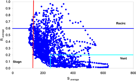
Figure 1. scatter plot of the hourly recirculation factor R vs. transport distance S and the corresponding classification according to Allwine and Whiteman (1994).

Results of the PCA (PC scores) are now combined with the obtained integral quantities. In Figure 2 it can be seen that negative PC1 and PC3 scores (i.e., very low along and across mountain wind speed values respectively), are observed under stagnation conditions, indicating calm flows as expected. This is especially true for PC3 where all scores are negative. Some moderate positive values of PC2 were correlated with stagnant conditions in accordance with the results found elsewhere (Halios et al., 2012): such PC2 scores are observed under open anti-cyclonic synoptic systems, which usually lead to calm conditions. Yet, the majority of PC2 scores are negative indicating stagnant conditions under overcast skies or night time periods.

FIGURE 2

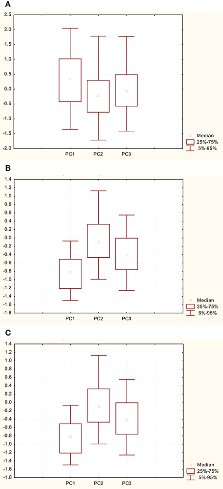
Figure 2. Box-plot of the PC scores under recirculation conditions (A) stagnation conditions (B) and ventilation conditions (C).

Ventilation conditions mainly correlate with positive PC1 and PC3 scores, associated with intense along and across mountain flows respectively. It should be noticed that in many cases positive PC1 scores are related with low or negative PC3 scores, when the dominant wind flow is along the mountain axis, and the across the mountain component is weak. The correlation coefficient between positive PC1 and PC3 scores for ventilation conditions is −0.4, and an example of such a case is shown in Figure 5B. There does not seem to be any preferable correlation between ventilation conditions and PC2 scores.

Recirculation is related mainly with flows parallel to the mountain axis, indicating mainly sea-breezes. Sea breezes have been reported to this location, with wind direction parallel to the mountain axis (Helmis et al., 1987, 1995). On the other hand, recirculation conditions are sometimes related with moderate flows perpendicular to the mountain axis, and most probably refer to other, local flows which develop in the vicinity of the mountain (e.g., katabatic flows studied in Helmis and Papadopoulos, 1996).

Geometric Structures

In Figures 3A,B, the percentage of occurrences of recognized structures in the temperature and wind fields is presented. The percentage of occurrences is the number of structures identified for each category divided by the maximum number of possible events in the data set. One striking difference between the two datasets is that the temperature field appears much better organized than the wind speed. In particular, all wind speed structures are less than 1% of the maximum theoretical number of events; the percentage is higher than 1% for all temperature structures. Following Belušić and Mahrt (2012) we propose that pressure fluctuations and shear instabilities act to smooth out the large momentum gradients, thus leading to less shapes in the wind speed field than in the temperature field. Percentage of (positive or negative) sine and step shapes are always higher than the corresponding percentage of (positive or negative) ramp-cliff or cliff-ramp shapes, again in accordance with Belušić and Mahrt (2012). A striking exception is the large percentage of positive cliff-ramp shapes in the temperature field, where 3.1% of the maximum theoretical number of events are cliff-ramp shapes against 1, 1.3, and 1.4% for ramp-cliff, step and sine shapes respectively. It has been proposed in several studies that within the turbulence scales, the preference of some specific geometric shapes is related with certain physical mechanisms, e.g., ramp and cliff structures in the temperature field are related with sharp assymetrical thermals and/or intermittent turbulence in stable conditions, whilst sines are related with smooth wave-like motions in the stable boundary layer (e.g., Belušić and Mahrt, 2012). For the larger scales as the one discussed here, the reason for the dominance of some shapes against the others is not quite clear. Yet, it is perhaps of interest to notice that for turbulence scales, cliff-ramp shapes with positive gradient are usually observed under stable conditions (Barthlott et al., 2007); and in our study the large percentage of these cases is observed during night time (see next section). This perhaps indicates to the development of this particular type of stratification in this environment.

FIGURE 3

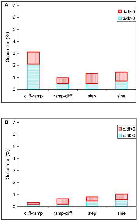
Figure 3. The percentage of recognized temperature (A) and wind speed (B) events relative to the theoretically maximum number of events.

In Belušić and Mahrt (2012) study it was concluded that the ratios of ramps, cliffs and step to sine occurrences were almost constant for all scales, being close to 0.2–0.3 for ramps and cliffs and higher than (or around to) unity for step shapes. Our results show that the step/sine ratios are indeed close to unity (0.9 and 0.8 for wind and temperature fields respectively); ramp-cliffs to sine are lower than unity (0.7 and 0.6 for wind speed and temperature fields respectively), but the cliff-ramp to sine ratio vary significantly, being 2.2 for temperature and 0.3 for wind speed time series. Apparently the deviation of the behavior of cliff ramp to sine ratio from the results found in Belušić and Mahrt (2012), reflects the high percentage of positive cliff-ramp shapes mentioned above. At this stage it is not clear what the reason is for the dominance of the positive ramp cliffs in the temperature time series.

Statistics

In Tables 2, 3 the percentage of the identified shapes (separated in positive and negative gradients) is presented according to the day period (night-time or day-time), the status of the flow field (ventilation, stagnation, recirculation or intermediate) and the dominant surface pattern (Principal Component Scores).

TABLE 2

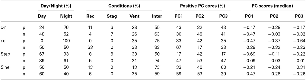
Table 2. Statistics of the identified temperature shapes according to the day period, status of the flow field and the dominant surface pattern.

TABLE 3

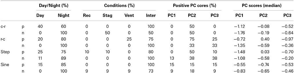
Table 3. Statistics of the identified wind speed shapes according to the day period, status of the flow field and the dominant surface pattern.

For the temperature structures (Table 2), mixed conditions are observed in terms of the flow fields and dominant surface pattern; several structures are under ventilation conditions, some under recirculation conditions and only a few under stagnant conditions.

The ramp-cliffs with negative gradient are observed under several recirculation conditions which in turn are related to enhanced along-mountain wind speed. For the turbulence scales this structure is associated with unstable conditions (Barthlott et al., 2007); contrary to this, in our study this structure is related with negative PC2 scores which occur either during night time, or under low pressure systems and fronts (Halios et al., 2012). Fifty two percent of these cases occur during night time. Thus, it is apparent that in the mesoscale region this particular structure is not related with the same physics that dominates turbulence scales.

Cliff-ramp with positive gradients and ramp-cliff with negative gradients are related with stable conditions in turbulence scales (Barthlott et al., 2007). Here, these structures appear mainly during night time (76 and 100% of the cases respectively), and correspond to negative PC1 and PC3 scores, indicating a weak flow field. This is especially true for the ramp-cliffs with a positive gradient (100% of the cases occur in night), which are observed under the total absence of recirculation conditions. It can be seen that there is a percentage of positive PC1 and PC3 scores (33 and 25% for PC1 and PC3 respectively) under temperature positive ramp-cliffs, which correspond to ventilation conditions. It is perhaps surprising that there are no stagnation conditions under this category; the very high percentage of unrecognized flows during this category could be an indication of the sensitivity of the method to the strong mountainous terrain. Further investigation of this issue would be of interest, but it is outside the scope of this article.

Positive step and negative sine shapes tend to appear during day time and they are related with enhanced ventilation values. Negative step and positive sine structures do not show a clear preference for the period of day, the flow or the temperature pattern. Exception to this, is the positive sine shape for which the ventilation cases are few and are related with the across mountain wind speed and low SR and T values, indicating weak local flows that develop during night time.

In contrast to the results of the temperature structures, it is apparent that uniform weak conditions dominate across all the wind structures (Table 3). The vast majority of the wind speed structures appears during night time, and consequently are related to negative PC2 score. They are also occurring under calm conditions (high negative PC1 and PC3 scores): it is characteristic that out of the 64 detected cases only one structure was observed under ventilation conditions. This is in line with the situations observed elsewhere in turbulent scales (e.g., Belušić and Mahrt, 2012). An exception is the positive step shapes, where some cases were observed under recirculation conditions.

Case Studies

In this section, structural shapes detected during 2 days are presented, and the corresponding meteorological conditions are analyzed in some detail.

The first case refers to the period 0:00 LST 14/3–2:00 LST 15/3 (Figures 4A,B, 5A). During the first night a cliff- ramp structure appears at 0:00 (Figure 5A) under a weak variable flow from the southern sector (intermediate conditions- Figure 4A). In the following morning, during a sunny winter day, PC2 scores gradually start to rise, leading to a maximum during midday. Between 11:00 and 17:00 LST a circulation with the characteristics of a sea-breeze develops: in Figure 4A a steady flow from the west-south-west sector with enhanced wind speed values (maximum value 2 ms⁻¹) can be observed, accompanied by a slight reduction of the temperature and enhancement of the relative humidity (Figure 4B). In previous studies flows with these characteristics were identified as sea-breezes (Helmis et al., 1995). Both the recirculation factor and PC1 scores during this period capture the sea-breeze event (e.g., relatively high values of Ri and PC1 scores). Two structures are observed in the temperature field during this period: a negative step structure (Figure 6C) appears between 15:00 and 16:00 LST, possibly associated with the sea breeze front, and followed by a positive cliff-ramp structure right afterwards (Figure 6A). After 19:00 LST a weak south flow is established again, which leads to stagnant conditions (S_i < 120 km) at 2:00 LST on 15/2. At that time negative ramp-cliff structures appear to both the temperature and wind fields (Figures 6B,D). In general, wind structures with negative gradients are associated with deceleration (the steeper part of the structure decreases) thus it is apparently related with divergence in the flow field according to Taylor's hypothesis (Belušić and Mahrt, 2012).

FIGURE 4

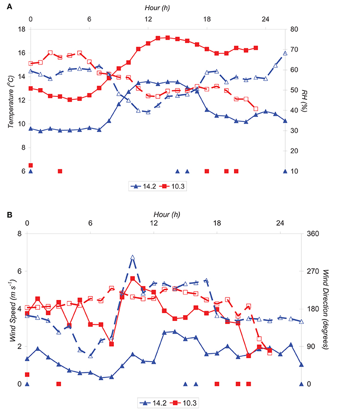
Figure 4. Time series of (A) mean hourly temperature (continuous lines with closed symbols) and relative humidity (dashed lines with open symbols) and (B) wind speed (continuous lines with closed symbols) and wind direction (dashed lines with open symbols) for the periods 0:00 14/2–2:00 15/2 (blue lines with triangles), and 0:00–23:00 10/3 (red lines with squares). At the bottom side of the two plots the hours when geometrical shapes were observed are indicated with closed symbols: blue triangles for 14/2, and red squares for 10/3.

FIGURE 5

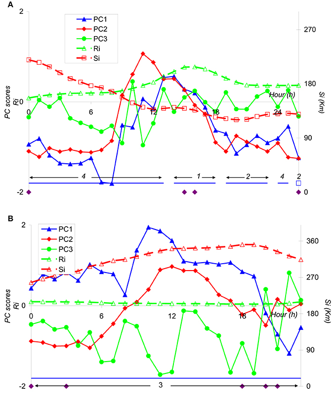
Figure 5. Time series of Principal Component scores and the main Integral quantities during (A) 0:00 14/2–2:00 15/2, and (B) 10/3. PC1–PC3 are denoted with continuous blue lines with triangles, and red lines with diamonds respectively, and wind run (Si) and recirculation factor (Ri) with dashed red and blue lines. At the bottom side of the two plots the hours when geometrical shapes were observed are indicated with diamonds and the categorization of the wind flow categories are also presented as: 1- recirculation, 2- stagnation, 3- ventilation and 4- intermediate conditions.

FIGURE 6

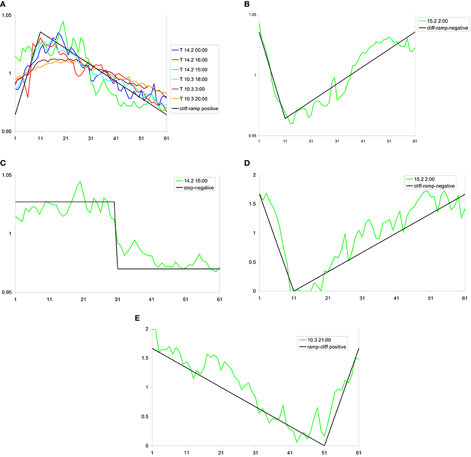
Figure 6. Geometrical structures appeared during the case studies. In the temperature field: cliff-ramps with positive (A) and negative gradient (B), and negative step shapes (C). In the wind speed field: negative cliff-ramp (D) and positive ramp-cliff (E). For temperature and wind speed series the mean has been subtracted in every case, while the geometric shapes are shown in arbitrary values. The time stamp is shown on the legend.

The second case is the 10/3, when constant winds blow from the south-south west sector throughout the day, leading to ventilation conditions (Figures 4A,B, 5B). Two positive cliff-ramp shapes are observed in the temperature field at 0:00 and 3:00 LST (Figure 6A). Interestingly enough, relative humidity during the night has the same pattern as during 14/2 (Figure 4A). After the sunset two more positive ramp-cliff shapes are observed in the temperature field (18:00, 20:00 LST), and the following hour (21:00 LST) one positive ramp-cliff in the wind speed field occurs (Figure 6E). It is interesting to note than even though ventilation conditions prevail during the whole day, the flow field has changed in the evening as indicated by the positive PC2 and negative PC1 scores. Thus, the leading circulation is now perpendicular to the mountain axis, is associated with an increase in the temperature and decrease in the relative humidity (Figure 5A), and is probably related with the development of a moderate down-slope circulation; the developed structure indicates an accelerated flow (positive gradient). Such down-slope circulations were observed in the past (Helmis and Papadopoulos, 1996).

Discussion and Conclusions

A recently developed simple linear technique, for the detection of basic shapes in meteorological time series was applied in the wind speed and temperature data of the time scale of 1 h measured at a location where a wide range of meso-scale flows have been identified in the past. Step changes, cliff-ramp, ramp-cliff and wave-like signals were identified, and it was found that the temperature field appears much better organized than the wind field. Cliff-ramp structures are dominant in the temperature time series.

The occurrence of structural shapes was related with the dominant flow patterns by applying Principal Component Analysis and analysis of integral quantities (wind run and recirculation factor) to the data. As integral quantities are true measures of the transport of a plume only under idealized homogeneous wind conditions it was argued that for this reason the large portion of flow conditions was not categorized. Nevertheless, 25% of the cases were categorized as ventilation conditions, 7% as recirculation and only 3% as stagnant conditions.

The temperature positive cliff-ramps and ramp-cliffs that within turbulence scales are related with stable conditions appear mainly during night time and under weak flow field. Temperature step and sine structures do not show a clear preference for the period of day, flow or temperature pattern. On the contrary, uniform stable, weak flow conditions dominate across all the wind speed structures.

A detailed analysis of the flow field during two case studies revealed that structural shapes might be part of larger flow structures, such as a sea-breeze front or down-slope winds. During stagnant conditions structural shapes that were associated with deceleration of the flow were observed, whilst during ventilation conditions shapes related with the acceleration of the flow.

It has been pointed out that coherent structures detected in humidity time series above forests or fields can be very important since they potentially control the mass exchange between the lower and upper layers (Krusche and De Oliveira, 2004). Coherent structures in humidity time series were not examined here since the vegetation cover was rather low.

As a future work, it would be of interest to compare the method applied here with conditional sampling techniques that are commonly used to identify coherent structures in the boundary layer. Then, it would become clearer how the structural shapes identified with the methodology applied here, correspond to the coherent structures analyzed in literature. In that frame, the methodology presented in Kang et al. (2014) is of particular interest. In that study, events were identified in noisy time series but without any pre-assumed characteristics of events in terms of their magnitude, geometry, or periodicity.

With the widespread availability of meteorological information from Automatic Weather Stations being easily accessible to the meteorological community, it is suggested here that the methods employed in this study could also apply to common meteorological datasets from other environments, giving more insight to the physics behind the structures developed in the meso-scale region. Also, combined application of these methods to sets of meteorological and air quality data easily available (e.g., concentrations of common pollutants such as CO, NO_x PM₁₀ etc. measured with commercial analyzers), would provide valuable information of the conditions that dominate diffusion of air pollution in the urban environment.

Conflict of Interest Statement

The authors declare that the research was conducted in the absence of any commercial or financial relationships that could be construed as a potential conflict of interest.

Acknowledgments

The author would like to acknowledge Mr. N. Kaltsounidis for data collection and Dr. Danijel Belusic for his constructive comments. The constructive comments of the two reviewers are acknowledged.

References

Allwine, K. J., and Whiteman, C. D. (1994). Single-station integral measures of atmospheric stagnation, recirculation and ventilation. Atmos. Environ. 28, 713–721.

Google Scholar

Barthlott, C., Drobinski, P., Fesquet, C., Dubos, T., and Pietras, C. (2007). Long-term study of coherent structures in the atmospheric surface layer. Bound. Lay. Meteorol. 125, 1–24. doi: 10.1007/s10546-007-9190-9

CrossRef Full Text | Google Scholar

Belušić, D., and Mahrt, L. (2012). Is geometry more universal than physics in atmospheric boundary layer flow? J. Geophys. Res. 117:D09115. doi: 10.1029/2011JD016987

CrossRef Full Text | Google Scholar

Boppe, R. S., Neu, W. L., and Shuai, H. (1999). Large-scale motions in the marine atmospheric surface layer. Bound. Lay. Meteorol. 92, 165–183.

Google Scholar

Campanharo, A. S. L. O., Ramos, F. M., Macau, E. E. N., Rosa, R. R., Bolzan, M. J. A., and Sá, L. D. A. (2008). Searching chaos and coherent structures in the atmospheric turbulence above the Amazon forest. Philos. Trans. R. Soc. A. 366, 579–589. doi: 10.1098/rsta.2007.2118

Pubmed Abstract | Pubmed Full Text | CrossRef Full Text | Google Scholar

Gao, W., Shaw, R. H., and Paw, U. R. T. (1989). Observation of organized structure in turbulent flow within and above a forest canopy. Bound. Lay. Meteorol. 47, 349–377.

Google Scholar

Halios, C. H., Helmis, C. G., Flocas, H. A., Nyeki, S., and Assimakopoulos, D. N. (2012). On the variability of the surface environment response to synoptic forcing over complex terrain: a multivariate data analysis approach. Meteorol. Atmos. Phys. 118, 107–115. doi: 10.1007/s00703-012-0209-5

CrossRef Full Text | Google Scholar

Helmis, C. G., and Papadopoulos, K. H. (1996). Some aspects of the variation with time of Katabatic flow over a simple slope. Q. J. R. Meteorol. Soc. 122, 595–610.

Google Scholar

Helmis, C. G., Papadopoulos, K. H., Kalogiros, J., Soilemes, A. T., and Asimakopoulos, D. N. (1995). The influence of the background flow on the evolution of the Saronic Gulf Sea Breeze. Atmos. Environ. 29, 3689–3701.

Google Scholar

Helmis, C. G., Asimakopoulos, D. N., Deligiorgi, D. G., and Lalas, D. P. (1987). Observations of sea-breeze fronts near the shoreline. Bound. Lay. Meteorol. 38, 395–410.

Google Scholar

Higgins, C. W., Froidevaux, M., Simeonov, V., Vercauteren, N., Barry, C., and Parlange, M. B. (2012). The effect of scale on the applicability of taylor's frozen turbulence hypothesis in the atmospheric boundary layer. Bound. Lay. Meteorol. 143, 379–391. doi: 10.1007/s10546-012-9701-1

CrossRef Full Text | Google Scholar

Jollife, I. T. (2002). Principal Component Analysis, 2nd Edn. New York, NY: Springer.

Kaimal, J. C., and Businger, J. A. (1970). Case studies of a convective plume and a dust devil. J. Appl. Meteorol. 9, 612–620.

Google Scholar

Kallos, G., Kassomenos, P., and Pielke, R. A. (1993). Synoptic and mesoscale weather conditions during air pollution episodes in Athens Greece. Bound. Lay. Meteorol. 62, 163–184.

Google Scholar

Kang, Y., Belusic, D., and Smith-Miles, K. (2014). Detecting and classifying events in noisy time series. J. Atmos. Sci. 71, 1090–1104. doi: 10.1175/JAS-D-13-0182.1

CrossRef Full Text | Google Scholar

Kikuchi, T., and Chiba, O. (1985). Step-like temperature fluctuations associated with inverted ramps in a stable surface layer. Bound. Lay. Meteorol. 31, 51–63.

Google Scholar

Koch, S. E., Feltz, W., Fabry, F., Pagowski, M., Geerts, B., Bedka, C., et al. (2008). Turbulent mixing processes in bores and solitary waves deduced from profiling systems and numerical simulation. Mon. Weather Rev. 136, 1373–1400. doi: 10.1175/2007MWR2252.1

CrossRef Full Text | Google Scholar

Krusche, N., and De Oliveira, A. P. (2004). Characterization of coherent structures in the atmospheric surface layer. Bound. Lay. Meteorol. 110, 191–211. doi: 10.1023/A:1026096805679

CrossRef Full Text | Google Scholar

Lykossov, V. N., and Wamser, C. (1995). Turbulence intermittency in the atmospheric surface layer over snow-covered sites. Bound. Lay. Meteorol. 72, 393–409. doi: 10.1007/BF00709001

CrossRef Full Text | Google Scholar

Mahrt, L. (2010). Common microfronts and other solitary events in the nocturnal boundary layer. Q. J. R. Meteorol. Soc. 136, 1712–1722. doi: 10.1002/qj.694

CrossRef Full Text | Google Scholar

Serafimovich, A., Thomas, C., and Foken, T. (2011). Vertical and horizontal transport of energy and matter by coherent motions in a tall spruce canopy. Bound. Lay. Meteorol. 140, 429–451. doi: 10.1007/s10546-011-9619-z

CrossRef Full Text | Google Scholar

Stull, R. (1988). An Introduction to Boundary Layer Meteorology. Dordrecht: Kluwer Academic Publishers, 666.

Google Scholar

Taylor, R. J. (1958). Thermal structures in the lowest layers of the atmosphere. Aust. J. Phys. 11, 168–176.

Google Scholar

Thomas, C., and Foken, T. (2006). Organised motion in a tall spruce canopy: temporal scales, structure spacing and terrain effects. Bound. Lay. Meteorol. 122, 123–147. doi: 10.1007/s10546-006-9087-z

CrossRef Full Text | Google Scholar

Wesson, K. H., Katul, G. G., and Siqueira, M. (2003). Quantifying organization of atmospheric turbulent eddy motion using nonlinear time series analysis. Bound. Lay. Meteorol. 106, 507–525. doi: 10.1023/A:1021226722588

CrossRef Full Text | Google Scholar

Wilks, D. S. (2006). Statistical Methods in the Atmospheric Sciences, 2nd Edn. Oxford, UK: Academic Press.

Zaman, K. B. M. Q., and Hussain, A. K. M. F. (1981). Taylor hypothesis and large-scale coherent structures. J. Fluid Mech. 112, 379–396.

Google Scholar