Weather types across the Maritime Continent: from the diurnal cycle to interannual variations

1. Introduction and Motivation

The atmospheric circulation exhibits a broad spectrum of motions. Multiple-flow regimes have been used to help understand large-scale, persistent and recurrent atmospheric patterns in mid-latitudes (Mo and Ghil, 1988; Vautard and Legras, 1988; Kimoto, 1989; Vautard, 1990; Michelangeli et al., 1995; Ghil and Robertson, 2002). Weather types (WT) have been employed extensively to diagnose and describe such regimes. This approach, however, has been used less often in the tropics (Pohl et al., 2005; Moron et al., 2008; Lefèvre et al., 2010), where space-time filtering has typically been used in order to focus on specific temporal scales—such as the intraseasonal one of 20–60 days associated with the Madden-Julian Oscillation (MJO) (Madden and Julian, 1971)—and removing the annual cycle is standard practice. The latter approach may be misleading when the annual cycle is modulated in phase or amplitude, since these modulations may be aliased into both shorter and longer time scales (Moron et al., 2012). Such aliasing might be particularly problematic in the tropics, where seasonal migrations of the intertropical convergence zone (ITCZ) and monsoon circulations represent a large fraction of the total variability.

We present, therefore, results of weather typing across the Maritime Continent (MC), and show that WTs computed using dynamical cluster analysis of unfiltered, daily, low-level winds do provide a unified and flexible view of the scale interactions. The MC provides a good example where multiscale interactions amongst various phenomena produce a particularly rich spectrum of atmospheric variations (Hendon, 2003; Chang et al., 2005a; Juneng and Tangang, 2005; Moron et al., 2010; Qian et al., 2010, 2013; Rauniyar and Walsh, 2011; Robertson et al., 2011). The asymmetrical annual cycle of the Asian-Australian monsoon (Chang et al., 2005a) provides a planetary-scale picture of the NW–SE movement of the ITCZ from Southeast Asia, in May–September, to Northern Australia in January-February. The huge amount of heat within the deep surface mixed layer of the Western Pacific Warm Pool, just east and north of Papua New Guinea, as well as the complex topography—with mountainous and flat islands of varying sizes dispersed across waters usually warmer than 28°C—lead to deep convection on small-to-regional scales, in association with the diurnal cycle (Qian, 2008; Rauniyar and Walsh, 2011; Teo et al., 2011) and with mountain and sea breezes (Qian et al., 2010, 2013). The MC and the Western Pacific are also located at the longitudes where the MJO reaches its highest amplitude in austral summer (Hendon and Liebmann, 1990; Wheeler and Hendon, 2004; Matthews and Li, 2005), a region that is also the western pole of the Pacific's Walker circulation and the Southern Oscillation (Bjerknes, 1969; Klein et al., 1999; Hendon, 2003).

At the interannual time scale, the MC thus plays a central role in the El Ni~no–Southern Oscillation (ENSO), with warm events usually associated with large-scale subsidence and low-level easterly anomalies (Klein et al., 1999; Hendon, 2003; McBride et al., 2003). Previous analyses showed that MC rainfall anomalies associated with ENSO are strongly modulated spatially across the annual cycle (Hendon, 2003; Juneng and Tangang, 2005) and that the onset of the austral-summer monsoon, between September and November (Haylock and McBride, 2001; Moron et al., 2009), is a key stage in this modulation, due to the difference in the way that anomalies and basic state are superimposed on either side of this stage. MC rainfall thus modifies the local air-sea coupling (Hendon, 2003), as well as the amplitude of the diurnal cycle and of the sea and mountain breezes (Qian et al., 2010, 2013). Our previous work (Moron et al., 2010; Qian et al., 2010, 2013) demonstrated that a quiescent-flow WT is key to understanding why ENSO causes wet anomalies over the central mountains of Java but dry anomalies over the plains during the monsoon season (Rauniyar and Walsh, 2011); this WT is more frequent during El Ni~no years and leads to an enhancement of the diurnal cycle of precipitation and of land-sea breeze circulation.

The goal of this paper is two-fold: (i) to build a unified picture of the impacts of ENSO and MJO on daily rainfall and circulation variability over the MC by using daily circulation regimes as the dynamical cross-scale interaction mechanism; and then (ii) to rely on the concepts of dynamical systems theory to interpret the multi-WT picture of the multi-scale interactions so obtained. We consider ENSO, MJO and the seasonal cycle as external forcings on regional atmospheric dynamics over the MC, and wish to determine to what extent these forcings change the nature of the regional dynamical attractor, rather than just causing certain parts of it to be visited more or less often (Ghil and Childress, 1987; Palmer, 1998; Ghil and Robertson, 2002). This determination has implications for sub-seasonal to seasonal predictability to the extent that these two distinct ways of affecting the regional dynamics imply different contributions to its predictability, as well as to its representation in numerical models.

We investigate this fundamental question in terms of WTs, and use observational datasets and reanalyses to quantify the extent to which ENSO, the MJO and the seasonal cycle are associated with changes in WT frequency vs. changes in the WT patterns. By identifying each WT with distinctly different diurnal-cycle behavior, we seek to span the range of scales from diurnal to interannual.

2. Materials and Methods

2.1. Data

Our weather typing approach is based on daily winds at 850 hPa from the second version of the NCEP reanalyses (Kanamitsu et al., 2002), for the years 1979–2013, during the 1 September to 30 April season, and within the window (15°S–15°N, 90°E–160°E). The 850 hPa wind field was shown in our previous work (Moron et al., 2010) to provide a good description of monsoonal WTs over the MC, and we extend the dataset here to cover the whole MC archipelago, and the complete austral-summer monsoon season.

In order to analyze WT relationships with convection, we employ interpolated daily outgoing longwave radiation (OLR) from the NOAA (Liebmann and Smith, 1996) dataset for the same space and time windows. We also use 3-hourly and daily estimated rainfall from TRMM 3b42 (Huffman et al., 2007; Chen et al., 2013, version 7) available on a 0.25° × 0.25° grid from January 1st, 1998, until the end of 2013. Units are converted from mm/hr to 1/10 mm/day and rainfall values are cube rooted to decrease skewness. Daily rainfall is available for only 15 complete seasons, from 1998/1999 on. All other atmospheric datasets have 242-day seasons, from 1 September to 30 April, over 34 years, with leap days removed, that is 242 days/year × 34 years = 8228 days.

2.2. Statistical methods

Before going into technical details, we present a broad picture of the overall methodology. We first extracted daily WTs from unfiltered low-level daily winds using dynamical clustering, also known as the k-means method (Michelangeli et al., 1995; Ghil and Robertson, 2002). The goal is to provide a coarse-grained view of the regional-scale atmosphere's phase space, by considering in principle all time scales from daily to decadal. The smallest spatial scales are nevertheless filtered out by considering only the leading Empirical Orthogonal Functions (EOFs) and their corresponding Principal Components (PCs).

The k-means clusters localize high concentrations of points in the phase subspace spanned by these EOFs. Their centroids are given by time averaging the low-level winds over all the days that belong to a given cluster and they define each distinct WT. Similar composites of OLR and rainfall over the days assigned to each cluster are then built to investigate the relationships between each low-level circulation type and large-scale convection or local-scale daily (and sub-daily) rainfall. Following the many previous studies cited in the previous section, we refer to the resulting patterns as “weather types” since they allow an interpretation of local rainfall variability in terms of regional-scale circulation and convection patterns.

Next, we investigate the impact of three key drivers of MC climate variability on the occurrence frequency and flow patterns of these WTs, namely the seasonal cycle, the MJO and ENSO. Their impacts are quantified using conditional probability, composites of raw and anomalous low-level winds and OLR, and multinomial logistic regression, with respect to the time series of these drivers. The goal is to separate the impact of these drivers on the recurrence or persistence of the WTs from their impacts on the spatial patterns thereof. Lastly, we analyze the diurnal cycle of local-scale (0.25°) rainfall to look at scale interactions and assess the ability of the WTs to capture any systematic impact on a shorter time scale, which is not explicitly resolved by the dynamical clustering of daily fields.

The daily gridded wind data are first standardized using the long-term mean and standard deviation. The initial dimension of the dataset is then reduced by applying an EOF analysis that retains 75% of the total variance in the 26 leading PCs. The k-means method partitions iteratively the ensemble of 8228 days into k clusters in such a way as to minimize the sum of variances within clusters (Diday and Simon, 1976). The first step of dynamical clustering is the random selection of k days from the 8228 days in the 26-dimensional subspace.

These initial seeds are taken as the cluster centers, and each daily circulation map is then assigned to the nearest center, according to Euclidean distance. The centroid of each of the k clusters is then taken as the cluster center in the second step, and the same procedure is repeated until the sum of intra-cluster variance stops decreasing, within a given tolerance.

The optimal number of clusters is determined—without removing the mean seasonal cycle—by using a red-noise test defined in Michelangeli et al. (1995). The 8228 days in the 26-dimensional subspace are classified 1000 times, each time starting from a different random seed. The partition having the highest mean similarity with the 999 other ones is kept. A classifiability index CI, shown in Figure 1 as a blue line with open circles, measures the average similarity within the 1000 sets of clusters and equals exactly 1 only if all 1000 partitions are identical, i.e., if the initial choice of random seeds has no impact on the final partition. The statistical significance of CI is tested by generating 100 classifications in exactly the same way as for the observed daily winds, projected onto the 26 leading PCs, except that one classifies red-noise processes having the same autocorrelation at a 1-day lag as the leading 26 PCs. The red-noise CIs are sorted in ascending order and the 90^th value gives the one-sided 90^th level of significance, shown as the red line in Figure 1.

FIGURE 1

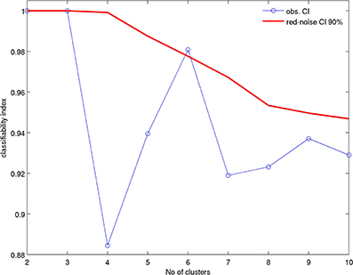
Figure 1. Classifiability index CI (Michelangeli et al., 1995) of the k-means, with k = 2 to 10 clusters, for the clustering of zonal and meridional daily 850 hPa winds; the dataset is 242 days from September 1st to April 30st in the 34 seasons from 1979–80 to 2012–13. The zonal and meridional winds are standardized to zero mean and unit variance and the k-means clustering is applied to the 26 leading principal components (PCs) that capture at least 75% of the entire variance. The red solid line is the one-sided 90% significance level from 100 red-noise simulations.

The impact of the seasonal cycle, ENSO, and MJO on the WTs' frequency and pattern is analyzed by computing composite counts and maps for different phases of the respective cycle. The significance of the anomalies is tested using a battery of non-parametric and Monte Carlo tests.

For the ENSO-phase composite maps associated with a particular WT, we use a Kolgomorov-Smirnov (KS) test to quantify the distance between the empirical cumulative distribution function of the subset of days making up the WT–ENSO composite, and the cumulative distribution function of the whole sample of 8228 days. The KS test is non-parametric and is hence preferable to the use of a Student's t-test. We compute independently for each grid point the KS test and complement it by a global (or field) significance test (Livezey and Chen, 1983) to estimate the significance of the difference between, for example, cold and warm ENSO events. The null hypothesis of such a global test is that the WT pattern associated with cold events is identical to that of the warm ones. This procedure is carried out for warm and cold ENSO phases, as well as for the eight MJO phases.

In order to test the impact of the ENSO and MJO on WT frequency, we used a permutation bootstrap by sampling a random set of years, in case of warm and cold ENSO events, or reshuffling yearly WT sequences as well as blocks of WT sequences. The impact of the seasonal cycle, ENSO, and MJO on the WTs' frequency is also estimated using multinomial logistic regression (cf. Gloneck and McCullagh, 1995; Guanche et al., 2014).

In this exercise, cross-validated regression models are built to “predict” WT frequency, using one, two or all of our three predictors. Consider the daily sequence {z_i : i = 1, …, N} of WTs over the N = 8228 days that can potentially take one of K nominal (i.e., unordered) categories and a time series {x_i : i = 1, …, N} of a predictor; here there are K = 6 categories and the possible predictors are the seasonal cycle, ENSO and MJO variations. The nominal values of z_i are converted into an N × K matrix Y of zeroes, except for the observed WTs, which are categorized as ones, that is, for each day, y_i = 1 for the observed WT and y_i = 0 for the 5 remaining unobserved WTs.

In the following, π_ik is the probability of the k^th WT, given a set of predictors x_i,

$\begin{array}{cc}{\pi }_{ik}=\mathrm{Pr}(y_i=k|x_i),& (1)\end{array}$

i.e., x_i could be a time series of scalars or of vectors, ${\overrightarrow{x}}_i=(x_i^j;j=1,\dots ,J)$, for J = 1,2 or 3, given the total number of our external forcings. This probability could be related to the set of x_i's through a set of K − 1 baseline WT logits. Taking k* as the baseline category, the model is

$\begin{array}{cc}\log \frac{{\pi }_{ik}}{{\pi }_{i{k}^{\ast }}}=\alpha +{\displaystyle \sum _{j=1}^{j=J}{\beta }_j{x}_i^j,\text{ with }k\ne k^{\ast }};& (2)\end{array}$

here α is a constant and the β_j's are the coefficients of each predictor variable.

Each coefficient β_j can be interpreted as the increase of log-odds of falling into k^th WT vs. the (k*)^th one that would result from a one-unit increase in the j^th predictor, while holding the other predictors constant. The accuracy of the model fit is independent of the WT chosen as the baseline.

The maximum likelihood estimator $\widehat{\beta }$ of β is calculated using the MATLAB function mnrfit. To estimate the model-based WT probability ${\widehat{\pi }}_i$ from $\widehat{\beta }$, the back transformation from Equation (2) is given by

$\begin{array}{cc}{\widehat{\pi }}_{ik}=\frac{e^{(\alpha +x_i{\widehat{\beta }}_k)}}{1+{\displaystyle {\sum }_{j\ne k^{\ast }}{e}^{(\alpha +x_i{\widehat{\beta }}_j)}}}\text{ for }k\ne k^{\ast },\text{ and}& (3)\end{array}$

$\begin{array}{cc}{\widehat{\pi }}_{i{k}^{\ast }}=\frac{1}{1+{\displaystyle {\sum }_{j\ne k^{\ast }}{e}^{(\alpha +x_i{\widehat{\beta }}_j)}}}\text{ for }k=k^{\ast }.& (4)\end{array}$

The fit is estimated vs. a saturated model in which π was estimated independently for i = 1, …, N. The deviance G² for comparing any model to a saturated one is given by

$\begin{array}{cc}{G}^2=2{\displaystyle \sum _{i=1}^N{\displaystyle \sum _{k=1}^K{y}_{ik}\log \frac{y_{ik}}{{\widehat{\pi }}_{ik}}}}.& (5)\end{array}$

We test various combinations of predictors—amongst the seasonal cycle, ENSO and MJO—in Section 3.2. The change Δ_G² in the deviance of Equation (5) serves to estimate the significance of the inclusion of added predictors relative to a “null” model that uses only an independent term β₀ as predictor or to a “parent” model that includes one or more predictors, up to J − 1, less than its “child”; for example, a “parent” model could include ENSO alone as a predictor, while a “child” could include both ENSO and MJO as predictors, i.e., in this case J = 2.

The statistic Δ_G² follows a chi-square distribution with δ_p × (k − 1) degrees of freedom, where δ_p is the difference in the number of predictors. The accuracy of the fit is also computed by cross-validation, i.e., the $\widehat{\beta }$'s are learned using 33 years of data, while $\widehat{\pi }$ is computed for each day of the remaining season using Equations (3, 4). We cannot expect to simulate properly the exact temporal sequence at the daily time scale, since only the annual (i.e., the seasonal cycle), interannual (i.e., ENSO) and sub-seasonal, 20–60-day (i.e., MJO) variations are explicitly considered.

We thus filtered out the shortest time scales in observed and hindcast WT sequences, by considering a running window of 11 days centered on the target day to get the 11-day mean of each $\widehat{\pi }$ and y and then the highest mean as yielding the predicted and observed WT's for the target day so that a contingency table between observed and predicted WTs could be set up. We tested various window sizes (from 7 to 21 days) to compute the mean and it yields similar results (not shown). The side effect of this choice is that some WTs are never predicted to occur, due to a systematic under-estimate of the standard variation of $\widehat{\pi }$, i.e., each daily value tends to its long-term mean, i.e., close to 1/6, and is thus never sufficiently high to be the maximum of the six $\widehat{\pi }$'s.

3. Results

3.1. Weather Types: Mean Seasonal Cycle and Mean Atmospheric Pattern

Figure 2 illustrates the rich multiscale atmospheric variations across the MC during 1982–1984; the OLR index, defined as the spatial average of the OLR on (96.25°E–121.25°E, 6.25°S–6.25°N), is in the upper panel and the wind index, defined as the spatial average of the 850-hPa zonal wind on (96.25°E–121.25°E, 11.25°S–1.25°S) is in the lower one. The lowest OLR values in Figure 2A occur at the end of the calendar year. A large interannual variation occurs between the strong warm ENSO event in 1982–83, with suppressed deep convection over the MC, and the weak cold event in 1983–84, with enhanced deep convection there. Fast variations are superimposed on this seasonal and interannual variability, with a broad bandwidth mostly under 10 days.

FIGURE 2

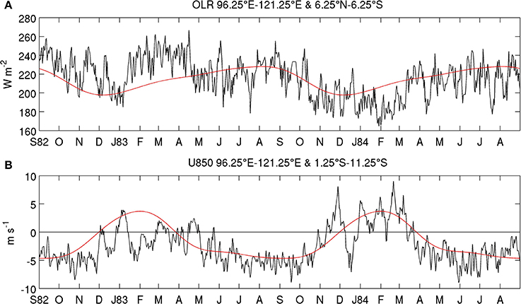
Figure 2. Time evolution of the outgoing longwave radiation (OLR) and zonal winds. Plotted are the spatial average of (A) daily OLR on (96.25°E–121.25°E, 6.25°S–6.25°N) in Wm⁻²; and (B) daily zonal wind on (96.25°E–121.25°E, 11.25°S–1.25°S) in ms⁻¹ (black lines) over two seasonal cycles, from 1 September 1982 to 31 August 1984. The long-term daily mean, low-pass filtered with a recursive Butterworth filter (cut-off = 90 days) is added as a red line. The ticks on the abcissa refer to the first day of each month.

The wind index in Figure 2B shows an asymmetric alternation between westerlies (i.e., WNW monsoon) that coincide with the austral summer monsoon, from early December to early April, and easterlies (i.e., trade-winds) during the rest of the year. As for the OLR index, the austral summer monsoon winds are clearly weaker in 1982–83 than in 1983–84, while there are pronounced intraseasonal fluctuations associated with the MJO (Madden and Julian, 1971; Wheeler and Hendon, 2004; Rauniyar and Walsh, 2011). These intraseasonal variations in zonal winds are at times as large as those associated with the mean annual cycle, for instance during November–December 1983 (Figure 2B).

We proceed with the WT classification in order to better understand the way that these large variations on different time scales occur. A significant peak at the one-sided 90% level appears for k = 6 in Figure 1. This number of WTs is one greater than in (Moron et al., 2010) but we consider here a larger spatial window and extend the analysis until the end of April, vs. February in (Moron et al., 2010), to include the decaying phase of the austral summer monsoon. Note also that considering 60 leading PCs (not shown), rather than 26 only, captures at least 90% of the total variance, rather than 75%, and still leads to the same results as those shown here, namely the days are clustered into the same WTs in 98% of cases.

The mean seasonal cycle of the frequency of occurrence of the six WTs (Figure 3) suggests that they can be interpreted first of all as snapshots of the mean annual cycle, consisting of an asymmetric alternation (Chang et al., 2005a) between the austral and boreal summer monsoons. The austral summer monsoon is exemplified by WT 4 with WTs 3 and 5 occurring during this season as well. WT 1 occurs almost exclusively before the austral summer monsoon, until early November, while WT 2 and 6 occur either in its early or late stages.

FIGURE 3

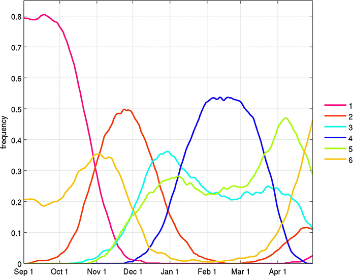
Figure 3. Mean seasonal cycle of the frequency of occurrence of the weather types (WTs). The daily frequency is low-pass filtered with a 31-day running mean.

The predominance of the annual cycle is also visible in the total-field composites of low-level winds and OLR in Figure 4. WT 1 in panel (a) is associated with the end of boreal summer, with ESE winds and high OLR south of the equator. The low OLR values associated with deep convection tend to progressively shift southeastward in WTs 2–4 (Figures 4B–D) and the low-level winds tends to veer to the WNW over almost the whole MC south of the Equator in WTs 3–4. WT 4 in panel (d) is most prevalent from early January to mid-March and its ITCZ reaches the southernmost location, touching Australia, with strong WNW winds that extend to Cape York, Queensland. WT 5 in Figure 4E still exhibits NE winds north of the Equator but the winds are now weaker over the MC and large-scale deep convection weakens relative to WTs 3–4 with poles over west-central Indonesia and New Guinea. Following (Moron et al., 2010), we refer to this WT as the “quiescent” one. WT 6 in panel (f) shows increased ESE winds south of the Equator all across the MC, while the ITCZ begins its northward migration.

FIGURE 4

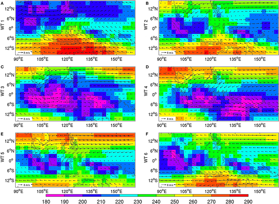
Figure 4. Mean raw OLR (shadings in Wm⁻²) and 850 hPa winds (vectors) for (A) WT 1, (B) WT 2, (C) WT 3, (D) WT 4, (E) WT 5, (F) WT 6 defined using k-means clustering of the standardized anomalies of 850 hPa winds projected onto the leading 26 EOFs for 1 September 1979 to 30 April 2013, while using the extended austral-summer (September to April) seasons only.

3.2. Weather Types: Interannual and Sub-Seasonal Variability

The temporal sequences of WT occurrences (not shown) confirm the strong seasonal component seen in Figures 3–4; their statistics are given in Table 1. Before the start of the austral summer monsoon, WT 1, which is the most persistent WT, tends to alternate with WT 6 and, to a lesser extent, with WT 2. During the austral summer season, WTs 3–5 alternate almost equiprobably, even though WT 4 leads to the longest spells. WT 3 and 5 are the most intermittent ones on the interannual time scale and also the least persistent at the intraseasonal ones. For example, WT 3 can be almost absent during a whole season, as in 1986/87, 1989–1992 and 2001/02 or occur frequently, as in 1998/99. Likewise, WT 5 does not occur at all in 1998/99, yet it is present on 102 days during the preceding 1997/98 season.

TABLE 1

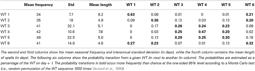
Table 1. Mean statistics of the length and transitions between the six WTs.

3.2.1. Interannual variability

An obvious candidate to explain interannual variations in WT occurrences and related atmospheric anomalies is ENSO. We analyze ENSO effects on the modulation of WT occurrences first and then on WT spatial patterns. The temporal evolution of WTs is studied for the 10 warmest—1982/83, 1986/87, 1987/88, 1991/92, 1994/95, 1997/98, 2002/03, 2004/05, 2006/07, 2009/10—and the 13 coldest—1984/85, 1985/86, 1988/89, 1995/96, 1998/99, 1999/2000, 2000/01, 2005/06, 2007/08, 2008/09, 2010/11, 2011/12, 2012/13—ENSO events, based on December–February mean sea surface temperature (SST) anomalies in the Ni~no 3.4 box (190°E–240°E, 5°S–5°N) being above 0.5°C and below −0.5°C, respectively. The remaining 11 years are referred to hereafter as “neutral.” The composite variations of WT frequency are computed within running 31-day windows and we use a permutation test that samples randomly 1000 times 10, 11, and 13 seasons in the 34 years to assess their significance (Figure 5).

FIGURE 5

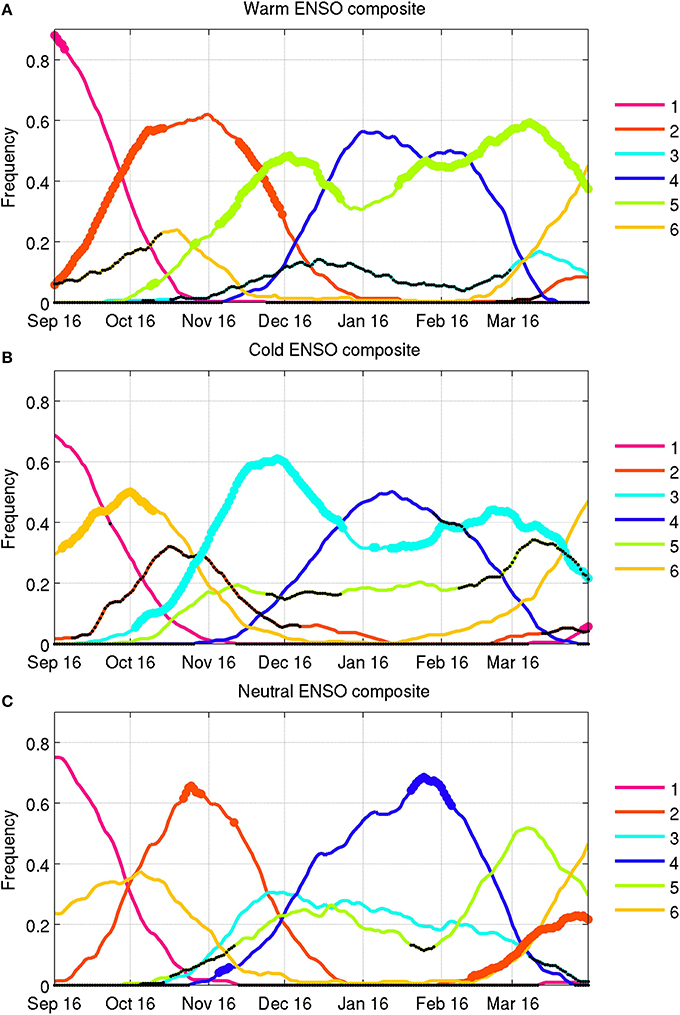
Figure 5. WT composites in running 31-day windows, classified by (A) warm, (B) cold and (C) neutral ENSO events. These are defined as the mean December–February SST anomalies in the Ni~no 3.4 box lying above +0.5°C (warm), below −0.5°C (cold), and between −0.5°C and +0.5°C (neutral) relative to the 1979/80-2012/13 mean. The dots—large and colored for positive and small and black for negative frequency deviations—indicate statistical significance at the two-sided 95% level as tested by 1000 random permutations of the observed yearly sequence of WTs.

Warm ENSO events (Figure 5A) are dominated by WT 1, followed by a large frequency increase of WT 2 until mid December. The core of the austral summer monsoon is almost equally dominated by WT 4 and the largely quiescent WT 5, which is significantly more frequent than usual. WT 3 occurs significantly less frequently than expected during the austral summer monsoon, with always <15% of days. The cold ENSO events (Figure 5B) are mostly related to an increased frequency of WT 3, especially around November-December and also in February-April. WT 2, and secondarily WT 5, occur less frequently than usual. The correlation between the September-April averaged Ni~no 3.4 SST index and seasonal WT frequency equals 0.34, with p−value = 0.06 according to a random-phase test (Janicot et al., 1996), 0.54 (p−value < 0.01), −0.76 (p−value < 0.01), 0.16 (p−value = 0.17), 0.81 (p−value < 0.01) and −0.57 (p−value < 0.01) for WTs 1–6, respectively.

These results suggest that ENSO strongly modulates both the persistence and the recurrence of WTs. Moreover, the neutral years (Figure 5C) do not show large anomalies and the seasonal evolution is then close to the long-term mean—except for, usually short, spells of excess of WT 2 around mid-November and in March-April and WT 4 after mid-November and around mid-February.

We next investigate whether there are significant changes in WT pattern during the different ENSO phases. Figure 6 shows composite WT anomalies for the warm (left column) and cold (middle column) ENSO events identified in the previous paragraphs, while the difference in WT pattern between warm and cold ENSO events is shown in the right column. The 850 hPa winds (vectors) and OLR anomalies (shading) are expressed as anomalies relative to the total-field composites of each WT shown in Figure 4. These anomaly maps thus express the ENSO effect on changes in WT pattern and they are plotted in color only when they are significant at the two-sided 95% level, according to our KS test.

FIGURE 6

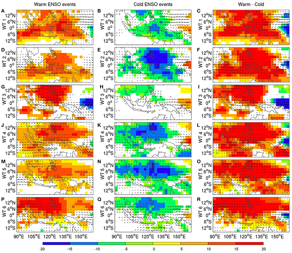
Figure 6. Mean OLR (shading in Wm⁻²) and 850-hPa wind anomalies: (left column) 10 warmest ENSO events; (middle column) 13 coldest ENSO events; and (right column) difference between warm and cold ENSO events for (A–C) WT 1, (D–F) WT 2, (G–I) WT 3, (J–L) WT 4, (M–O) WT 5, (P–R) WT 6. Warm and cold ENSO events are defined as in Figure 5. The OLR anomalies are shown in color only when they are significant at the two-sided 95% level according to the Kolmogorov-Smirnov (KS) test described in Section 3.2. The 850 hPa winds anomalies are plotted as vectors only when zonal or meridional winds are significant at the two-sided 95% level according to the KS test.

Large areas of significant ENSO impacts on WT pattern are visible, with El Ni~no tending to decrease convection and La Ni~na to increase it, broadly across all six WTs. To test globally the hypothesis whether the WTs patterns are significantly modulated by ENSO phase, the field significance of these composites is evaluated as follows: in place of the warm and cold years, respectively, 10 and 13 years are randomly chosen 1000 times and the KS-significant areas are computed for each of the three columns of Figure 6.

For the composite wind fields, the significant area is never reached by more than 10% of the random samples, except for the wind of WT 3 (=33% for the zonal and meridional components) in cold ENSO events, and for the wind of WT 5 (=14% for the zonal and = 11% for the meridional component), in warm ENSO events. For OLR, the significant area observed in warm and cold ENSO events is never reached by more than 8% of the random noise samples.

Our global KS tests thus confirm that the difference between WT patterns observed during cold vs. warm ENSO events cannot be attributed to sampling uncertainty, and that ENSO significantly modulates the WT patterns, in addition to WT frequency. This systematic modulation (right column of Figure 6) is nearly constant across the WTs, with an anomalous regional-scale divergence (convergence) at 850 hPa centered between Mindanao, Java and NW Australia, combined with anomalous subsidence (ascendance) over most of the MC, while a small area of enhanced (reduced) convection appears over the equatorial Pacific east of New Guinea, during warm (cold) ENSO events.

3.2.2. Sub-seasonal variability

At sub-seasonal scales, Figure 7 quantifies the impact on WT frequency of phase locking with the eight MJO phases—as defined by Wheeler and Hendon (2004) and used for predictive purposes by Kondrashov et al. (2013). In the upper panel, it is clear that the occurrence of the active-monsoon WTs 3 and 4 is favored during MJO phases 5–7, during which convection is enhanced from Indonesia to the western Tropical Pacific, while WTs 5 and 6—which represent weak, or break, monsoon episodes—occur more frequently during MJO phases 1–3, associated with enhanced convection mostly over the Indian Ocean (Wheeler and Hendon, 2004).

FIGURE 7

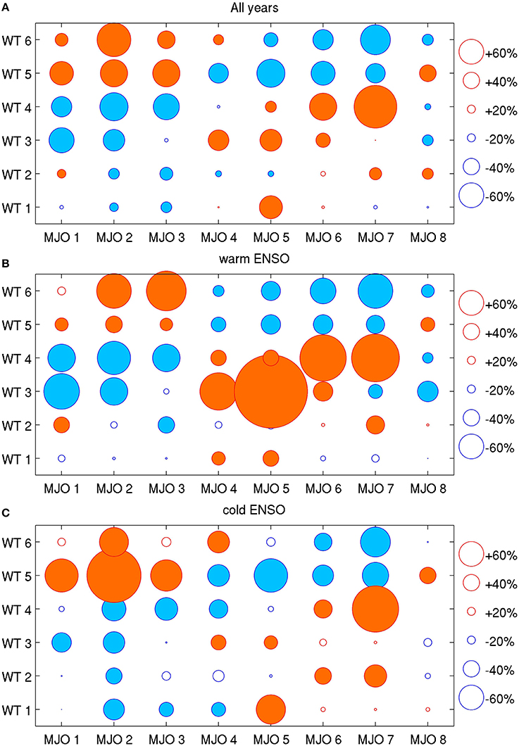
Figure 7. Phase locking of the WTs to the 8 phases of the MJO (Wheeler and Hendon, 2004; Kondrashov et al., 2013) expressed as anomalous conditional probability of WT occurrence during MJO phases. The filled orange and blue dots indicate significant positive and negative anomalies, respectively, at the two-sided 95% level, as tested by 1000 random permutations of the observed daily sequences of the WTs. (A) anomalies computed for all 34 seasons; and (B,C) anomalies discretized for the warm and cold ENSO events, respectively, defined as in Figure 5.

The anomalous WT frequencies were also computed for the 10 warm ENSO and 13 cold ENSO seasons in the middle and lower panels of Figure 7. The association between WT frequency and MJO phases is also seen, separately, in El Ni~no and La Ni~na years. However, the active-monsoon WTs 3 and 4 are more strongly suppressed in MJO phases 1–3 and more strongly favored in MJO phases 4–7 during El Ni~no episodes (middle panel). Thus, MJO forecasts may be of particular value during El Ni~no years for early warning of drought and flood episodes.

A KS test of significant changes in WT pattern was also performed for the 8 MJO phases, analogous to the one described for the ENSO phases in Figure 6. However, in the case of MJO, the result of the global field significance test was negative—the observed significant area is usually beaten by more than 10% of the random samples except for respectively 3 and 1 cases out of 48 (=6 WTs × 8 MJO phases) tests in zonal and meridional winds—i.e., there is usually no significant perturbation of the WT patterns by MJO phase.

The above analyses suggest that (1) the annual cycle exerts a strong control on WT occurrence; (2) ENSO events impact the frequency of WTs (mostly WT 2, 3, 5, and 6) as well as their patterns, through spatially homogeneous, sustained atmospheric anomalies across the MC—i.e., suppressed regional-scale convection during warm ENSO events—rather than changing the overall pattern of each WT; while (3) MJO impacts only the frequency of WTs. The relative impact of each of the three quasi-periodic forcings on WT frequency, and of their combinations, is estimated next, using a multinomial logistic regression.

3.2.3. Predictive models of WT frequency based on seasonal cycle, ENSO and MJO

Our goal here is to retrospectively forecast WT occurrence frequency, given perfect knowledge of these three regional climate drivers. We first construct two filtered daily time series to represent the seasonal cycle and Ni~no 3.4 SSTs, since the 8 MJO phases are already available from Wheeler and Hendon (2004). The seasonal cycle is estimated with the first PC of standardized anomalies of the zonal and meridional components of the 850-hPa wind, while keeping the seasonal cycle and analyzing the full year. The first PC is low-pass filtered with a recursive Butterworth filter of order 9 and with a cut-off = 1/90 cycle-per-day. The variability includes a quasi-regular seasonal cycle combined with a minor modulation at the interannual time scale related with ENSO variability: the correlation between the September–April average of PC 1 and the Ni~no 3.4 index is 0.63.

We remove the ENSO-related variance by linear regression as follows: A daily time series is created from the monthly SST anomaly of the Ni~no 3.4 index (NINO hereafter) by first sampling monthly values at a daily time scale and then filtering this time series with the same Butterworth filter as PC1 above. The Ni~no 3.4 effect is then removed from PC1 through linear regression and the extraction of the residual. The annual index so obtained is referred to hereafter as AN.

Table 2 shows the seven possible multinomial logistic regression models when using the three distinct predictors AN, NINO and MJO of daily WT occurrence. The “null” model (first row of the table) takes into account only an independent term and its deviance is analogous to the sum of squared errors in linear regression, providing a baseline for model comparison. All the changes in the model deviances Δ_G² between a nested model, i.e., adding one or more predictors, and a parent one, are statistically significant at the one-sided 99.9% level, according to a chi-squared test with 5 degrees of freedom (Guanche et al., 2014), where 5 equals the number of added predictors (=1 in our cases), by the number of WTs (= k) minus 1. Hence the addition of the predictors significantly improves the model fit.

TABLE 2

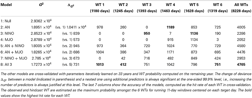
Table 2. Fitting diagnostic and cross-validated hit rates for different multinomial logistic models (Gloneck and McCullagh, 1995), including the three distinct predictors indicated in the first column (see text); the first model (“null”) includes only the intercept and is not cross-validated.

AN provides clearly the largest decrease of deviance, while MJO and NINO contribute roughly equally to this decrease. Considering the three predictors together improves the fit relative to the best model using two predictors, i.e., AN and NINO (fifth row of the table). In other words, the joint impact of AN, NINO and MJO provides the best fit of the observed sequences of daily WTs.

The cross-validated hit rates (rightmost 7 columns of the table) confirm the differential impact of the three predictors on the occurrence of each WT. NINO (third row in the table) is a major driver of the occurrence of WT 3 and WT 5 during the wet season, while WT 4 frequency is mostly affected by AN (row 2; cf. Figure 3). The marginal impact of MJO (row 4) is largest for WTs 4 and 5.

The joint impact of AN and MJO is rather similar to that of AN and NINO, except for WT 3, even though the marginal effects of NINO and MJO (rows 3 and 4) strongly differ, AN being the dominant one. The interannual variability of the WT probability is well-specified by the model including all three AN, NINO and MJO, with correlations between hindcast and observed seasonal frequency equal to 0.73 (WT 1), 0.50 (WT 2), 0.78 (WT 3), 0.66 (WT 4), 0.83 (WT 5) and 0.58 (WT 6), all values being significant at the one-sided 95% level according to a random-phase test (Janicot et al., 1996).

3.2.4. Filtering of WT patterns

Finally, we compare the interannual and sub-seasonal anomalies for each WT, with respect to the mean annual cycle calculated on a daily basis. The goal here is to separate the phenomena associated with each WT by filtering the contributions to the composite WT maps in Figure 4 from the interannual and sub-seasonal frequency bands. For example, if they were solely a reflection of ENSO impacts, then applying a high-pass sub-seasonal filter would yield near-zero anomalies for each WT. This analysis complements the previous ones, since we do not assume a priori the special role of ENSO or MJO, while the dominant driver of WT occurrence, i.e., the mean seasonal cycle, is filtered out.

The anomalies are computed as deviations between raw values (shown in Figure 4) and the mean seasonal cycle; they are then decomposed into two additive components, on either side of a period of 242 days—i.e., the length of the extended austral summer, September 1–April 30—by using a 9th-order recursive Butterworth filter with a cut-off frequency of (1/242) cycle/day. The composites for each of the two frequency bands are then plotted for each WT in Figure 8. Note that this analysis makes no distinction between the impacts of the respective oscillation on WT frequency vs. WT amplitude: it merely assesses the relative roles of ENSO and MJO in giving rise to these WTs.

FIGURE 8

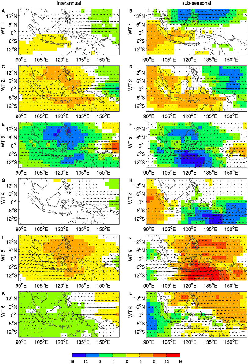
Figure 8. OLR (shadings in Wm⁻²) and 850 hPa winds: (left column) interannual and (right column) sub-seasonal anomalies associated with (A,B) WT 1, (C,D) WT 2, (E,F) WT 3, (G,H) WT 4, (I,J) WT 5 and (K,L) WT 6. The significance is computed by using 1000 random permutations of non-overlapping blocks of 22 days of daily WT sequences amongst the 34 years to account for the mean seasonal cycle, i.e., taken at the same stage of the cycle, and shown as color (OLR) and vectors (850-hPa wind) only when OLR, zonal or meridional components of the wind are above the two-sided 95% level of significance according to random permutations.

The pattern correlations between the interannually and sub-seasonally filtered WTs in Table 3 indicate substantial similarity in both OLR and wind anomalies, especially for WTs 2, 3, and 5. These three WTs are also the most variable in their frequency of occurrence at the interannual time scale (cf. Table 1).

TABLE 3

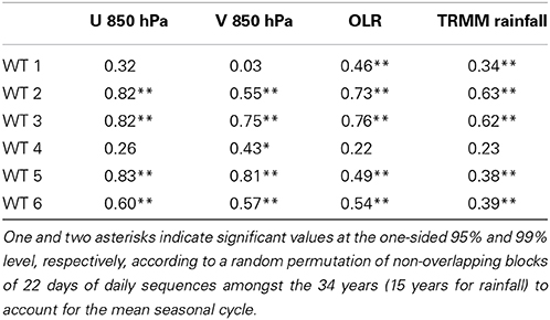
Table 3. Pattern correlation between the interannual and sub-seasonal anomalies associated with each WT shown in Figure 6.

Figure 8 shows that the anomalies are generally stronger in the sub-seasonal than in the interannual band. WT 3 is associated with anomalous low-level convergence and enhanced deep convection over Central Indonesia, while anomalous subsidence and therewith positive OLR anomalies, as well as increased low-level easterlies are observed over the Western Tropical Pacific. WT 5 shows an almost reversed pattern, with anomalous low-level divergence centered over New Guinea, accompanied by easterly anomalies and increased subsidence over most of Indonesia. WT 2 has some similarities with WT 5, except that anomalous low-level divergence, i.e., higher OLR, occurs between the South China Sea and Northern Australia.

The similarity between sub-seasonal and interannual components is less obvious for WTs 1, 4, and 6, which also tend to show rather weak interannual components (Table 3); this weakness suggests that these WTs do tend to be less excited by interannual forcing, and indeed the interannual variability of their frequency of occurrence tend to be small, cf. Tables 1, 3.

3.3. Weather Types: Associated Local-Scale Rainfall Anomalies

The analyses so far have focused on regional-scale anomalies. Downscaling to local-scale anomalies is now considered, using the 0.25° × 0.25° TRMM dataset (Huffman et al., 2007). We need to be cautious about these analyses since they refer to the second half of the period only and there are known biases in the TRMM remote-sensing data relative to in situ rain gages (Dinku et al., 2007).

As before, we decompose the rainfall anomalies according to time scale. This provides a measure of how interannual and sub-seasonal rainfall variability is described by changes in frequency and amplitude of daily WTs. We first computed interannual and sub-seasonal anomalies in rainfall as in Figure 8, after taking the cubic root of daily rainfall values to reduce skewness.

As for OLR and 850-hPa winds, there is a significant pattern correlation between interannual and sub-seasonal anomalies (Table 3). For each WT there is an expected broad-scale inverse relationship between OLR (Figure 8) and rainfall anomalies (Figure 9). However, this association does not hold everywhere, in particular not over islands. The quiescent WT 5, for example, is associated at sub-seasonal scales (Figure 8) with positive OLR anomalies—almost everywhere, except over the eastern Indian Ocean—but positive rainfall anomalies are observed over Sumatra, western Borneo, Java, and Sulawesi, especially at sub-seasonal scales (Figure 9). Note also that dipolar precipitation anomalies appear over Borneo and New Guinea, especially for WTs 3, 5, and 6. The positive rainfall anomalies tend to be located in the lee of the mountains, in particular along the northwest coast of Borneo and in central New Guinea. This “island wake” effect (Qian et al., 2013) may be associated with land-sea breeze enhancement on the mountains' lee side.

FIGURE 9

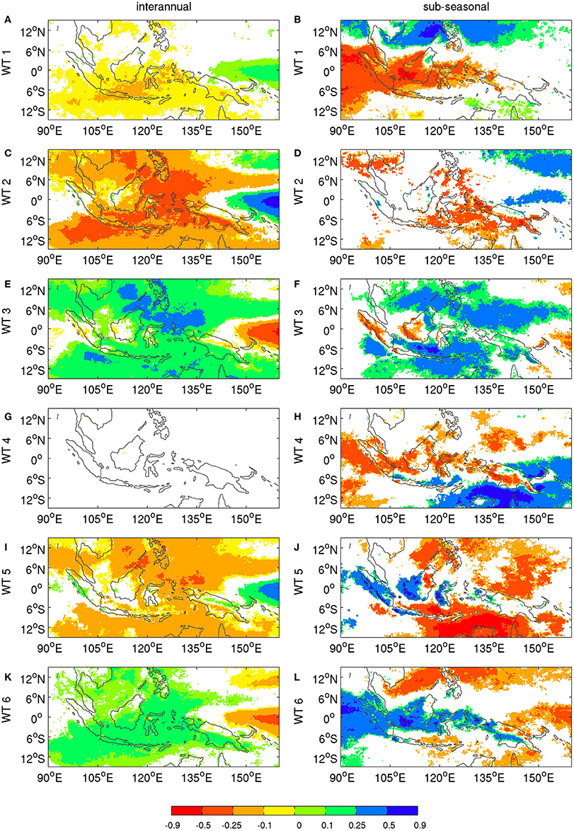
Figure 9. Same as Figure 8, except for daily rainfall from the TRMM 3b42 (version 7) dataset (Huffman et al., 2007). Rainfall data are available from 1998/1999 on only. Daily rainfall (in 1/10 mm/day) are cube rooted before the computation of climatological mean and anomalies. The significance is computed as in Figure 8, except that only 15 years are available for the randomizing of the sequences.

The relationship between OLR and small-scale rainfall anomalies is further investigated in Figure 10. OLR is first interpolated onto the much finer TRMM grid over the same time interval, from 1998/99 on, as daily rainfall. The anomalies relative to the mean seasonal cycle of daily means are then standardized to zero mean and unit variance and spatially averaged for the core region of the MC (94°E–125°E, 10°S–6°N).

FIGURE 10

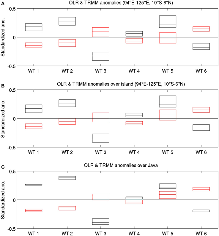
Figure 10. OLR (black) and TRMM rainfall (red) standardized anomalies relative to the mean seasonal cycle for each WT, from 1998/1999 on only. Daily rainfall values (in 1/10 mm/day) are cube-rooted before the computation of climatological mean and anomalies; median—central horizontal line, upper and lower quartiles—upper and lower limits of the box. (A) Whole MC core area; (B) islands only; and (C) Java only. The plot for the sea only (not shown) is practically indistindinguishable from panel (A). See text for details.

At this regional scale (Figure 10A), there is a broad anti-symmetry between OLR and rainfall anomalies, even though rainfall anomalies are closer to zero. Considering only the island points (Figure 10B) tends to weaken this anti-symmetry for WTs 2 and 3, where median rainfall anomalies tend to zero, and especially so for WT 5; in WT 5, OLR and rainfall anomalies are both positive, thus associating suppressed regional-scale deep convection with positive local-scale rainfall anomalies that could not be accurately captured by the OLR field's spatial resolution in our data. Such specifically asymmetric behavior of WT 5 appears also at even smaller scales, as seen over Java in Figure 10C.

3.4. Weather Types: Variations in the Diurnal Cycle

Diurnal-cycle variations are systematically analyzed for our six WTs by considering the 3-hourly mean rainfall at each grid point that corresponds to the climatological peak phase of the diurnal cycle; this peak occurs in the late afternoon to early night over islands and late night to early morning around islands, with no clear peak observed over open seas. The rainfall for the diurnal peak is standardized with respect to the mean seasonal cycle and averaged for each of our six WTs; the results are plotted in Figure 11.

FIGURE 11

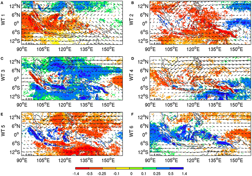
Figure 11. TRMM rainfall anomalies (shadings) for the peak of the diurnal cycle at each grid point and raw 850-hPa daily winds (vectors) for (A) WT 1, (B) WT 2, (C) WT 3, (D) WT 4, (E) WT 5, (F) WT 6. The TRMM anomalies are computed as the differences from the climatological daily mean. Maximum daily rainfall values (in 1/10 mm/day) are cube-rooted before the computation of climatological mean and anomalies. The significance is computed and plotted as in Figure 9; see text for details.

The local-scale significance is estimated using the same permutation method as the one employed for Figure 9. The peak phase of the diurnal cycle is enhanced with respect to climatology over Java in WT 5, as expected, but also over most of Sumatra, southwest Borneo, Sulawesi, and most of the Sunda islands (Figure 11E), while peak daily rainfall is significantly below climatology over most of the open seas, except off the western coasts of Sumatra and Borneo.

The positive rainfall anomalies over islands east of 105°E in WT 5 are not related to enhanced large-scale convection, but rather to the increased strength of the diurnal cycle at small spatial scales, when eastward anomalies are superimposed on the normal westerlies associated with the austral summer monsoon (Moron et al., 2010; Qian et al., 2010, 2013), as well as to local-scale SSTs (Hendon, 2003; Qian et al., 2013). This special phenomenon for the “quiescent” WT 5 may be explained by the inverse relationship between the monsoonal wind speed and the intensity of diurnal cycle, increasing sea-breeze and valley-breeze convergence toward the mountains during weak monsoon, thus brings forth more rainfall over the mountains than over the adjacent plains and seas (Moron et al., 2010; Qian et al., 2010).

4. Concluding Remarks

4.1. Summary

In this paper we have analyzed the characteristics of atmospheric variations over the Maritime Continent (MC) using the pattern recognition framework of weather typing. This framework has been extensively used for the extratropics (Mo and Ghil, 1988; Vautard and Legras, 1988; Kimoto, 1989; Vautard, 1990; Michelangeli et al., 1995; Ghil and Robertson, 2002) but less so in the tropics.

The MC shows a rich spectrum of temporal variations (Figure 2), including a strong seasonal cycle associated with the migration of the planetary-scale ITCZ. Our study focused on the austral summer monsoon, 1 September–30 April, for 34 seasons from 1979/80 to 2012/13. Six weather types (WTs) were obtained using k-means cluster analysis of unfiltered daily low-level wind fields (Figures 3, 4).

We interpreted these six WTs firstly as stages of the seasonal progression of the planetary-scale monsoon circulation (Figure 3) from the pre-monsoonal WT 1 through the core monsoonal WTs 3–5 and on to the post-monsoonal WT 6. The pre-monsoonal WT 1 and transitional WTs 2 are thus characterized by the low-level easterlies south of the equator that are common to both pre- and post-monsoonal stages.

Values of OLR below 210 Wm⁻² are restricted to the north of the equator in WT 1 and shifted toward two near-equatorial minima, between Sumatra and Borneo, on the one hand, and between New Guinea and the Western Tropical Pacific, on the other, in WTs 2 and 6 (Figure 4). Marked seasonal changes take place in November–March, with a progression toward the monsoonal WTs 3–5 accompanied by westerlies that are strongest in WT 4, but quiescent in WT 5, and the strongest deep convection occurring south of the equator. WT 4 corresponds to the peak of the austral summer monsoon with strong westerlies reaching Northern Australia and a clear equatorial westerly flow from Sumatra to the Western Pacific (Figure 4).

Using the WT framework, interannual and sub-seasonal variations lend themselves to interpretation in terms of changes in WT frequency of occurrence and their associated atmospheric anomalies at these scales (Figures 5–8). On the interannual time scale, the strongest anomalies are observed for WT 3, on the one hand, and WT 2 and 5, on the other: WT 3 (respectively WT 2 and 5) exhibits low-level anomalous convergence (respectively divergence) over eastern and/or central MC, along with enhanced (respectively suppressed) regional-scale deep convection (Figure 8). The interannual signal is weaker for the pre- and post-monsoon WTs 1 and 6, as well as for the peak WT 4 of the austral summer monsoon.

This behavior is consistent with the anomalies in WT frequency observed during ENSO events. Warm ENSO events are mostly associated with an increased occurrence of WT 1, followed by WT 2—which delays the regional-scale onset of the austral summer monsoon—and then by an increased frequency of the quiescent WT 5 during the rainy season; the latter corresponds to a superimposition of low-level easterly anomalies (Figure 6) upon the climatological westerlies associated with the austral summer monsoon (Figure 4). WTs 2 and 5 are associated with an enhanced diurnal cycle in the northern and southern MC, respectively, where synoptic winds are weak; weak winds lead to positive rainfall anomalies over some islands, or parts of islands, while large-scale subsidence promotes negative rainfall over most of the MC's inner seas (Figure 11). These results are consistent with our previous work (Moron et al., 2009, 2010; Qian et al., 2010, 2013), as well as with (Jourdain et al., 2013), who found that the anti-correlation between MC precipitation and the Ni~no 3.4 index in DJFM is more marked over ocean than over land in CMIP3 and CMIP5 model runs.

Cold ENSO events are not exactly symmetric, with more WT 6 episodes occurring just before the austral summer monsoon and especially more WT 3 than usual during the core of the rainy season. ENSO events do also modify the spatial pattern of WTs through the superposition of persistent anomalies associated with regional-scale anomalous subsidence (ascendance) during warm (cold) ENSO events (Figure 6).

On sub-seasonal time scales, the variation of WT frequencies is partly attributable to the MJO, with WTs 3–6 significantly locked with MJO phases. The sub-seasonal circulation anomalies are more pronounced amongst the WTs (Figure 8) but are similar to those on interannual time scales in their patterns, especially for WTs 2, 3, and 5. However, contrary to the effect of ENSO events, MJO does not appear to impact the WT patterns themselves significantly.

4.2. Discussion

Our results show that the WT framework can provide flexible tools to diagnose atmospheric anomalies across time scales, analyze potential predictability, and provide an easy way to spatially downscale any variable related to WT occurrence. Weather typing applied to unfiltered daily values covers in theory all time scales—from daily to interannual and interdecadal—i.e., up to the total number of years included in the analysis, equal here to 34 years. Of course, using EOF pre-filtering prior to the k-means clustering filters out the smallest and fastest variations. The reduction to a small set of WTs, equal here to six for 8228 days, also acts as a filter, while other clustering techniques (e.g., self-organizing maps) usually consider a larger set of situations, often more than 16, e.g., (Verdon-Kidd and Klem, 2009; Brown et al., 2010).

In any clustering, there is a trade-off between robustness and resolution. Transient mesoscale and synoptic-scale features, like the Borneo vortex (e.g., Chang et al., 2003, 2005b; Tangang et al., 2008) or individual tropical depressions or even cyclones (Chang et al., 2003) are obviously not captured by a small number of WTs, but this does not mean that WTs do not provide information on fast and small scales. As soon as one WT is associated with systematic and reproducible variations at any scale, this information is retrievable in the WT framework. It is the case here with the systematic modulation of the diurnal cycle over several islands or parts thereof—including Sumatra, western Borneo, Java, and Sulawesi—mostly in WT 5 and, at least, in sectors where a combination of sub-seasonal to seasonal variations and the annual cycle weakens the regional-scale winds and thus increases the diurnal-cycle amplitude (Moron et al., 2010; Qian et al., 2013).

In their recent study, Peatman et al. (2013) concluded that 80% of the MJO precipitation signal over the MC is accounted for by changes in the amplitude of the diurnal cycle, which responds over islands about 6 days in advance of the arrival of the main MJO convective envelope. They argue that frictional and topographic moisture convergence and relatively clear skies then combine with the low thermal inertia of the islands, to allow a rapid response in the diurnal cycle. According to our results, the “quiescent” WT 5 is responsible for the strong diurnal signal over islands, and it is most prevalent in MJO phases 1–3, when the MJO convective envelope is over the Indian Ocean (Figure 7). We argue that the quiescent large-scale winds of WT 5 allow the diurnal cycle to amplify, as described in Qian et al. (2010, 2013).

Although the MJO modulation of WT 5 is most marked during La Ni~na events (Figure 7C), this is tempered by the much less frequent occurrence of WT 5 during the cold phase of ENSO (Figure 5B), so that this MJO modulation of diurnal precipitation is less likely to be observed at that time.

An early dynamical interpretation of extratropical WTs, or planetary flow regimes (Legras and Ghil, 1985; Ghil and Childress, 1987), was in terms of fixed points of the governing flow equations. In the tropics, moist processes play a larger role than in mid-latitudes, and one can thus expect the need for more complex interpretations. Moreover, boundary forcing by SSTs in the tropics is much more important than in mid-latitudes. In particular, we found here that WTs can capture transient modes or systematic variations, such as the seasonal cycle. We have shown, in fact, that WTs can be interpreted, to first order, as fixed snapshots of the annual cycle, since this time scale was retained in our analysis and not filtered out at the outset, as is typically done.

Furthermore, it was possible to separate the atmospheric anomalies associated with each WT according to large-scale climate phenomena on both the interannual and sub-seasonal scale, namely as being affected by either ENSO or the MJO, respectively. For example, the broad-scale easterly anomalies observed in WTs 2 and 5 refer clearly to warm ENSO events, acting through large-scale subsidence over eastern Indonesia. Likewise we found that WT 5 is more phase-locked to MJO than WT 2 is. Such a data-adaptive, WT-mediated decomposition of time scales is complementary to the usual a priori selection that is provided by removing the mean annual cycle or by bandpass filtering. Our WT framework helps one also to interpret the phase shifts associated with the seasonal cycle as the delayed onset of the austral summer monsoon during warm ENSO events, an aspect that may be blurred when the seasonal cycle is filtered out a priori.

Returning to the conceptual framework of dynamical systems theory introduced in Section 1, we may conclude that the importance of “external” forcings—i.e., of ENSO, the MJO and the seasonal cycle—in the Tropics in general and in the regional dynamics of the MC in particular—requires the application of the broader and more flexible concepts of open, non-autonomous, and possibly random dynamical systems (cf. Ghil et al., 2008; Chekroun et al., 2011; Ghil, 2014) and references therein, while the more standard theory of closed, autonomous systems was largely sufficient for planetary-scale, extratropical phenomena (Ghil and Childress, 1987, Ch. 5). Thus, the seasonal cycle introduces a strong periodic modulation of the atmosphere's dynamical attractor over the MC, for which the six discrete WTs that occur in overlapping fashion at different stages of the monsoonal progression provide a robust “skeleton.” For the sake of brevity, we will not enter into the technical aspects of the time-dependent pullback attractors that are required to describe the behavior of non-autonomous systems, and only use the concepts loosely in order to interpret the present findings.

The occurrence frequency of certain WTs is significantly impacted from year to year by ENSO and sub-seasonally by the MJO, modulating in time the size and shape of the corresponding attractor basins. Sub-seasonal to seasonal predictability of circulation over the MC may be partially framed in terms of the strength of these frequency modulations. In addition, ENSO was shown to exert an influence on the spatial structure of circulation patterns for certain WTs, thereby modulating, on interannual time scales, the position that the pullback attractor's successive “snapshots” occupy in the system's phase space. This effect is not found for the MJO, whose impact appears to be purely on the WTs' frequency of occurrence.

The atmospheric Southern Oscillation limb of ENSO modulates the strength of the planetary-scale Walker Circulation, whose ascending branch is located over the MC. Thus, it is very plausible that ENSO would modulate the structure of the MC's pullback attractor on shorter spatial scales. While the MJO also has a large wavenumber-one component zonally, it is transient on the time scale of WT transitions and propagates through the MC; it is therefore to be expected that its impact on the WTs would be largely by modulating their frequency, with less impact on the overall attractor structure.

Besides the theoretical considerations above, the connection between daily weather conditions and large-scale climate drivers afforded by the WT framework is very useful from the applied climate perspective. For example, farmers in Western Java plant their first rice crop after monsoon onset in October–December, followed by a second crop, which they plant in May-June. The first is vulnerable to flooding in January-February, and the second to drought, especially if the monsoon onset is delayed by El Ni~no (Boer and Subbiah, 2005; Moron et al., 2009). The work presented here could help identify the atmospheric drivers of flood and drought events at local scale within specific WT daily sequences, which in turn may help develop sub-seasonal to seasonal forecasts that are more accurate and better tailored to the needs of farmers.

Conflict of Interest Statement

The authors declare that the research was conducted in the absence of any commercial or financial relationships that could be construed as a potential conflict of interest.

Acknowledgment

We thank F. Kucharski, F. Molteni, J. Shukla, and D. Straus for their valuable comments and suggestions on the preliminary stages of this paper, during the school and workshop on “Weather regimes and weather types in the tropics and extra-tropics: Theory and application to prediction of weather and climate” held in October 2013 at the International Centre for Theoretical Physics in Trieste. Three-hourly data from the TRMM 3b42 mission, version 7, have been downloaded free of charge from the map room site of the International Research Institute for Climate and Society (IRI; http://ingrid.ldgo.columbia.edu), while Reanalysis-2 and OLR daily data were downloaded free of charge from the Earth System Research Laboratory of NOAA's Physical Science Division (http://www.esrl.noaa.gov/psd/data/gridded/). Michael Ghil and Andrew W. Robertson were supported by MURI grant N00014-12-1-0911 from the Office of Naval Research, and Andrew W. Robertson also by the International Fund for Agricultural Development.

References

Bjerknes, J. (1969). Atmospheric teleconnections from the equatorial Pacific. Mon. Wea. Rev. 97, 163–172. doi: 10.1175/1520-0493(1969)097<0163:ATFTEP>2.3.CO;2

CrossRef Full Text | Google Scholar

Boer, R., and Subbiah, A. R. (2005). “Agricultural droughts in Indonesia,” in Monitoring and Predicting Agricultural Drought: A Global Study, eds V. S. Boken, A. P. Cracknell, and R. L. Heathcote (New York, NY: Oxford University Press), 330–344.

Google Scholar

Brown, J. R., Jakob, C., and Haynes, J. M. (2010). An evaluation of rainfall frequency and intensity over the Australian region in a global climate model. J. Clim. 23, 6504–6525. doi: 10.1175/2010JCLI3571.1

CrossRef Full Text | Google Scholar

Chang, C.-P., Liu, C.-H., and Kuo, H.-C. (2003). Typhoon Vamei: an equatorial tropical cyclone formation. Geophys. Res. Lett. 30. doi: 10.1029/2002GL016365

CrossRef Full Text | Google Scholar

Chang, C.-P., Harr, P. A., and Chen, H.-J. (2005b). Synoptic disturbances over the equatorial Souttime Continent during boreal winter. Mon. Wea. Rev. 133, 489–503. doi: 10.1175/MWR-2868.1

CrossRef Full Text

Chang, C.-P., Wang, Z., McBride, J., and Liu, C.-H. (2005a). Annual cycle of Southeast Asia Maritime Continent rainfall and the asymmetric monsoon transition. J. Clim. 18, 287–301. doi: 10.1175/JCLI-3257.1

CrossRef Full Text | Google Scholar

Chekroun, M. D., Simonnet, E., and Ghil, M. (2011). Stochastic climate dynamics: random attractors and time-dependent invariant measures. Physica D 240, 1685–1700. doi: 10.1016/j.physd.2011.06.005.

CrossRef Full Text | Google Scholar

Chen, Y., Ebert, E. E., Walsh, K. J. E., and Davidson, N. E. (2013). Evaluation of TRMM 3B42 precipitation estimates of tropical cyclone rainfall using PACRAIN data. J. Geophys. Res. 118, 1–13. doi: 10.1002/jgrd.50250

CrossRef Full Text | Google Scholar

Diday, E., and Simon, J. C. (1976). “Clustering analysis,” in Digital Pattern Recognition, Communication and Cybernetics, Vol. 10, ed K.S. Fu (Springer-Verlag), 47–94.

Dinku, T., Ceccato, P., Grover-Kopec, E., Lemina, M., Connor, S. J., and Ropelewski, C. F. (2007). Validation of satellite rainfall products over East Africa's complex topography. Int. J. Remote Sensing 28, 1503–1526. doi: 10.1080/01431160600954688

CrossRef Full Text | Google Scholar

Ghil, M. (2014). “A mathematical theory of climate sensitivity or, How to deal with both anthropogenic forcing and natural variability?,” in Climate Change: Multidecadal and Beyond, eds C. P. Chang, M. Ghil, M. Latif, and J. M. Wallace (London: World Scientific Publishing Co.; Imperial College Press).

Google Scholar

Ghil, M., and Childress, S. (1987). Topics in Geophysical Fluid Dynamics: Atmospheric Dynamics, Dynamo Theory and Climate Dynamics. New York; Berlin; Tokyo: Springer-Verlag. doi: 10.1007/978-1-4612-1052-8

CrossRef Full Text | Google Scholar

Ghil, M., and Robertson, A. W. (2002). “Waves” vs. “particles” in the atmosphere's phase space : a pathway to long-range forecasting? Proc. Natl. Acad. Sci. U.S.A. 99, 2493–2500. doi: 10.1073/pnas.012580899

Pubmed Abstract | Pubmed Full Text | CrossRef Full Text

Ghil, M., Chekroun, M. D., and Simonnet, E. (2008). Climate dynamics and fluid mechanics: natural variability and related uncertainties. Physica D 237, 2111–2126. doi: 10.1016/j.physd.2008.03.036

CrossRef Full Text | Google Scholar

Gloneck, G. F. V., and McCullagh, P. (1995). Multivariate logistic models. J. R. Stat. Soc. Ser. B 57, 533–546.

Google Scholar

Guanche, Y., Minguez, R., and Méendez, F. J. (2014). Autoregressive logistic regression applied to atmospheric circulation patterns. Clim. Dyn. 42, 537–552. doi: 10.1007/s00382-013-1690-3

CrossRef Full Text | Google Scholar

Haylock, M., and McBride, J. L. (2001). Spatial coherence and predictability of Indonesian wet season rainfall. J. Clim. 14, 3882–3887. doi: 10.1175/1520-0442(2001)014<3882:SCAPOI>2.0.CO;2

CrossRef Full Text | Google Scholar

Hendon, H. H. (2003). Indonesian rainfall variability: impacts of ENSO and local air-sea interaction. J. Clim. 16, 1775–1790. doi: 10.1175/1520-0442(2003)016<1775:IRVIOE>2.0.CO;2

CrossRef Full Text | Google Scholar

Hendon, H. H., and Liebmann, B. (1990). The intraseasonal (30–50 day) oscillation of the Australian summer monsoon. J. Atmos. Sci. 47, 2909–2923. doi: 10.1175/1520-0469(1990)047<2909:TIDOOT>2.0.CO;2

CrossRef Full Text | Google Scholar

Huffman, G. J., Adler, R. F., Bolvin, D. T., Gu, G., Nelkin, E. J., Bowman, K. P., et al. (2007). The TRMM multi-satellite precipitation analysis: Quasi-global, multi-year, combined-sensor precipitation estimates at fine scale. J. Hydrometeor. 8, 38–55. doi: 10.1175/JHM560.1

CrossRef Full Text | Google Scholar

Janicot, S., Moron, V., and Fontaine, B. (1996). Sahel drought and ENSO dynamics. Geophys. Res. Lett. 23, 515–518.

Google Scholar

Jourdain, N. C., Sen Gupta, A, Taschetto, A. S., Ummenhofer, C. C., Moise, A. F., and Ashok, K. (2013). The Indo-Australia monsoon and its relationship to ENSO and IOD in reanalysis data and the CMIP3/CMIP5 simulations. Clim. Dyn. 41, 3073–3102. doi: 10.1007/s00382-013-1676-1

CrossRef Full Text | Google Scholar

Juneng, L., and Tangang, F. (2005). Evolution of ENSO-related rainfall anomalies in SouthEast Asia region and its relationship with atmosphere-ocean variations in the Indo-Pacific sector. Clim. Dyn. 25, 337–350. doi: 10.1007/s00382-005-0031-6

CrossRef Full Text | Google Scholar

Kanamitsu, M., Ebisuzaki, W., Woollen, J., Yang, S.-K., Hnilo, J. J., Fiorino, M., et al. (2002). NCEP-DOE AMIP-II Reanalysis (R-2). Bull. Amer. Meteor. Soc. 79, 1631-1643. doi: 10.1175/BAMS-83-11-1631

CrossRef Full Text

Kimoto, M. (1989). Multiple Flow Regimes in the Northern Hemisphere Winter. Ph.D. thesis, University of California, Los Angeles.

Klein, S. A., Soden, B. J., and Lau, N.-C. (1999). Remote sea surface temperature variations during ENSO: evidence for a tropical atmospheric bridge. J. Clim. 12, 917–932. doi: 10.1175/1520-0442(1999)012<0917:RSSTVD>2.0.CO;2

CrossRef Full Text | Google Scholar

Kondrashov, D., Chekroun, M. D., Robertson, A. W., and Ghil, M. (2013). Low-order stochastic model and “past-noise forecasting” of the Madden-Julian oscillation. Geophys. Res. Lett. 40, 5305–5310. doi: 10.1002/grl.50991

CrossRef Full Text | Google Scholar

Lef&#x02018;evre, J., Marchesiello, P., Jourdain, N. C., Menkes, C., and Leroy, A. (2010). Weather regimes and orographic circulation. Marine Poll. Bull. 61, 413–431. doi: 10.1016/j.marpolbul.2010.06.012

Pubmed Abstract | Pubmed Full Text | CrossRef Full Text | Google Scholar

Legras, B., and Ghil, M. (1985). Persistent anomalies, blocking and variations in atmospheric predictability. J. Atmos. Sci. 42, 433–471.

Google Scholar

Liebmann, B., and Smith, C. A. (1996). Description of a complete (interpolated) outgoing longwave radiation dataset. Bull. Amer. Meteor. Soc. 77, 1275–1277.

Google Scholar

Livezey, R. E., and Chen, W. Y. (1983). Statistical field significance and its determination by Monte Carlo techniques. Mon. Wea. Rev. 111, 46–59.

Google Scholar

Madden, R. A., and Julian, P. R. (1971). Detection of a 40-50 day oscillation in the zonal wind in the Tropical Pacific. J. Atmos. Sci. 28, 702–708. doi: 10.1175/1520-0469(1971)028<0702:DOADOI>2.0.CO;2

CrossRef Full Text | Google Scholar

Matthews, A. J., and Li, H.-Y.-Y. (2005). Modulation of station rainfall over the Western Pacific by the Madden-Julian oscillation. Geophys. Res. Lett. 32, L14827. doi: 10.1029/2005GL023595

CrossRef Full Text | Google Scholar

McBride, J. L., Haylock, M. R., and Nicholls, N. (2003). Relationships between the Maritime Continent heat source and the El Ni no Southern Oscillation phenomenon. J. Clim. 16, 2905–2914. doi: 10.1175/1520-0442(2003)016<2905:RBTMCH>2.0.CO;2

CrossRef Full Text | Google Scholar

Michelangeli, R. A., Vautard, R., and Legras, B. (1995). Weather regimes: recurrence and quasi-stationarity. J. Atmos. Sci. 52, 1237–1256. doi: 10.1175/1520-0469(1995)052<1237:WRRAQS>2.0.CO;2

CrossRef Full Text | Google Scholar

Mo, K., and Ghil, M. (1988). Cluster analysis of multiple planetary flow regimes. J. Geophys. Res. 93, 927–952. doi: 10.1029/JD093iD09p10927

CrossRef Full Text | Google Scholar

Moron, V., Robertson, A. W., and Qian, J.-H. (2010). Local versus regional-scale characteristics of monsoon onset and post-onset rainfall over Indonesia. Clim. Dyn. 34, 281–299. doi: 10.1007/s00382-009-0547-2

CrossRef Full Text | Google Scholar

Moron, V., Robertson, A. W., and Boer, R. (2009). Spatial coherence and seasonal predictability of monsoon onset over Indonesia. J. Clim. 22, 840–850. doi: 10.1175/2008JCLI2435.1

CrossRef Full Text | Google Scholar

Moron, V., Robertson, A. W., and Ghil, M. (2012). Impact of the modulated annual cycle and intraseasonal oscillation on daily-to-interannual rainfall variability across monsoonal India. Clim. Dyn. 38, 2409–2435. doi: 10.1007/s00382-011-1253-4

CrossRef Full Text | Google Scholar

Moron, V., Robertson, A. W., Ward, M. N., and Ndiaye, O. (2008). Weather types and rainfall over Senegal. Part I: observational analysis. J. Clim. 21, 266–287. doi: 10.1175/2007JCLI1601.1

CrossRef Full Text | Google Scholar

Palmer, T. N. (1998). Nonlinear dynamics and climate change: Rossbys legacy. Bull. Amer. Meteor. Soc. 79, 1411–1423. doi: 10.1175/1520-0477(1998)079<1411:NDACCR>2.0.CO;2

CrossRef Full Text | Google Scholar

Peatman, S. C., Matthews, A. J., and Stevens, D. P. (2013). Propagation of the Madden–Julian Oscillation through the Maritime Continent and scale interaction with the diurnal cycle of precipitation. Quart. J. R. Meteorol. Soc. 140, 814–825. doi: 10.1002/qj.2161

CrossRef Full Text | Google Scholar

Pohl, B., Camberlin, P., and Roucou, P. (2005). Typology of pentad circulation anomalies over the Eastern Africa – Western Indian ocean region, and their relationship with rainfall. Clim. Res. 29, 111–127. doi: 10.3354/cr029111

CrossRef Full Text | Google Scholar

Qian, J.-H. (2008). Why precipitation is mostly concentrated over islands in the Maritime Continent. J. Atmos. Sci. 65, 1428–1441. doi: 10.1175/2007JAS2422.1

CrossRef Full Text | Google Scholar

Qian, J.-H., Robertson, A. W., and Moron, V. (2010). Multi-scale interaction between ENSO, monsoon and diurnal cycle over Java, Indonesia. J. Atmos. Sci. 67, 3509–3523. doi: 10.1175/2010JAS3348.1

CrossRef Full Text

Qian, J.-H., Robertson, A. W., and Moron, V. (2013). Diurnal cycle in weather regimes and rainfall variability over Borneo associated with ENSO. J. Clim. 26, 1772–1790. doi: 10.1175/JCLI-D-12-00178.1

CrossRef Full Text | Google Scholar

Rauniyar, S. P., and Walsh, K. J. E. (2011). Scale interaction of the diurnal cycle of rainfall over the Maritime Continent and Australia: influence of the MJO. J. Clim. 24, 325–348. doi: 10.1175/2010JCLI3673.1

CrossRef Full Text | Google Scholar

Robertson, A. W., Moron, V., Qian, J.-H., Chang, C.-P., Tangang, F., Aldrian, E., et al. (2011). “The maritime continent monsoon,” in The Global Monsoon System: Research and Forecast, 2nd Edn., eds C.-P. Chang, Y. Ding, G. N.-C. Lau, R. H. Johnson, B. Wang, and T. Yasunari (New Jersey: World Scientific Publishing Co.), 85–97. doi: 10.1142/9789814343411_0006

CrossRef Full Text

Tangang, F., Juneng, L., Salimun, E., Vinayachandran, P. N., Seng, Y. K., Reason, C. J. C., et al. (2008). On the roles of the northeast cold surge, the Borneo vortex, the Madden-Julian oscillation and the Indian ocean dipole during the extreme 2006/2007 flood in southern Peninsular Malaysia. Geophys. Res. Lett. 35. doi: 10.1029/2008GL033429

CrossRef Full Text | Google Scholar

Teo, C.-K., Koh, T. Y., Lo, J. C.-F., and Bhatt, B. C. (2011). Principal component analysis of observed and modeled diurnal rainfall in the Maritime Continent. J. Clim. 24, 4662–4675. doi: 10.1175/2011JCLI4047.1

CrossRef Full Text | Google Scholar

Vautard, R., and Legras, B. (1988). On the source of midlatitude low-frequency variability. Part II: nonlinear equilibration of weather regimes. J. Atmos. Sci. 45, 2845–2867. doi: 10.1175/1520-0469(1988)045<2845:OTSOML>2.0.CO;2

CrossRef Full Text | Google Scholar

Vautard, R., Mo, K. C., and Ghil, M. (1990). Statistical significance test for transition matrices of atmospheric Markov chains. J. Atmos. Sci. 47, 1926–1931.

Google Scholar

Vautard, R. (1990). Multiple weather regimes over the North Atlantic: analysis of precursors and successors. Mon. Wea. Rev. 118, 2056–2081. doi: 10.1175/1520-0493(1990)118<2056:MWROTN>2.0.CO;2

CrossRef Full Text | Google Scholar

Verdon-Kidd, D. C., and Klem, A. S. (2009). On the relationship between large-scale climate modes and regional synoptic patterns that drive Victorian rainfall. Hydrol. Earth Syst. Sci. 13, 467–479. doi: 10.5194/hess-13-467-2009

CrossRef Full Text | Google Scholar

Wheeler, M. C., and Hendon, H. H. (2004). An all-season real-time multivariate MJO index: development of an index for monitoring and prediction. Mon. Wea. Rev. 132, 1917–1932. doi: 10.1175/1520-0493(2004)132<1917:AARMMI>2.0.CO;2

CrossRef Full Text | Google Scholar