Quantifying tracer dynamics in moving fluids: a combined Eulerian-Lagrangian approach

Introduction

The mechanisms of transport in fluids are important to various fields such as physics and chemistry (e.g., Ban and Gilbert, 1975; Bird et al., 2007 and references within), as well as medicine and biology (e.g., Lih, 1975). Though transport occurs at various scales (Bird et al., 2007 and references within), the underlying processes are similar among different systems. Transport is often affected by turbulence, from blood flow to atmospheric and oceanic currents (Dewan, 2011). Turbulent transport remains challenging to study because of its non-linearity and episodicity. Here we present a combined Eulerian-Lagrangian approach that allows us to follow and quantify tracer dynamics in a turbulent fluid. As an example of its utility, we apply this method to the study of biological-physical interactions in a marine planktonic system.

Biological and physical processes interact strongly in the ocean, leading to an inhomogeneous distribution of marine life. Plankton, the lower trophic levels of this ecosystem, are strongly influenced by their environment. Planktonic ecosystems are composed of small organisms, phytoplankton and zooplankton, with a typical body size ranging from microns to millimeters, and, by definition, drift with the ocean currents. Phytoplankton comprise the first trophic level of the marine food web, using light and nutrients to grow. The second trophic level is composed of zooplankton feeding on phytoplankton. Thus, planktonic ecosystems are strongly structured by light and nutrient availability, but also by temperature, mixing and other physical processes.

Biological-physical (biophysical) interactions occur over a wide range of timescales (Stommel, 1963; Haury et al., 1978). At small scales (millimeters to few meters), biophysical interactions are rapid (minutes to hours) and involve phytoplanktonic physiological processes and predation. For example, small-scale turbulence affects nutrient uptake by phytoplankton cells, which in turn influences the size structure and species composition of the phytoplankton community (e.g., Kiørboe, 1993; Estrada and Berdalet, 1997). At the global scale (several thousands of kilometers), biophysical interactions determine biogeographic provinces, defined by climatological conditions (Longhurst, 1995). The California Upwelling Coastal Province represents one of these biogeographic regions. In the California Upwelling System, seasonal equatorward winds blow along the coast, leading to upwelling of cold, salty, nutrient-rich water in the nearshore region. This nutrient-rich water supports intense biological activity of planktonic ecosystems and enhanced fish production. Between the small scale and the global scale, the mesoscale (10 km to ~200 km) is characterized by two-dimensional vortex features known as eddies. These eddies last from a week to several months, and are often associated with enhanced biological activity compared to the surrounding oligotrophic waters (i.e., low nutrient concentration and limited biological activity) (e.g., Haury et al., 1978; The Ring Group, 1981).

Though biophysical interactions in the sea have been extensively investigated through in situ observations, in vitro experiments, and in silico analyses, most mechanisms remain unclear. In particular, the mechanisms associated with planktonic ecosystem variability in eddies and upwelling systems are still in debate. Oceanic Global Circulation Models (OGCMs) provide a key tool for studying such complex mechanisms. Given the monotonic improvements in computing resources, OGCMs are able to resolve increasingly complex biophysical interactions. These models produce massive amounts of numerical data that often require specialized tools for the identification, extraction, and quantification of features and dynamics. Here, we discuss how the combination of Lagrangian and Eulerian methods can help us understand the mechanisms driving planktonic dynamics in complex physical systems. In Section Modeling Biological-physical Interactions, we briefly describe these methods, and in Section Description of the Combined Eulerian-Lagrangian Approach, we explain why their combined use presents a useful and powerful approach. We illustrate this combined approach through case studies of eastern boundary upwelling systems (EBUS) in the last Section, Combined Eulerian-Lagrangian Analyses in EBUS.

Modeling Biological-physical Interactions

Biogeochemical models are able to describe the ecosystem with simple sets of biological dynamics translated into mathematical functions. Because plankton can be considered as a continuous property (present in large quantities in most oceanic systems), they can be mathematically modeled with box model structures. Such modeling consists in computing the transfers of nutrients (the biological fluxes) between the organic and inorganic components of the ecosystem (the biomass). These models can be very simple, e.g., with only Nutrient-Phytoplankton-Zooplankton (NPZ, e.g., Franks, 2002), or include complex biogeochemical cycling models with several N-, P-, or Z-compartments, additional detritus compartments (particulate or dissolved matter), and a variety of interconnections.

To study spatial patterns of plankton and assess complex biophysical interactions, these ecosystem models have been coupled with three-dimensional ocean circulation models. OGCMs represent a particularly powerful tool for studying the complex, non-linear biophysical interactions of planktonic ecosystems. In an Eulerian framework, the evolution of a tracer concentration can be described at each fixed point in space by the advection-diffusion equation:

$\frac{\partial C}{\partial \text{t}}+\overrightarrow{u}·\nabla C=Diffusion+Sources-\begin{array}{cc}Sinks& (1)\end{array}$

where C is the tracer concentration, the ∂/∂t operator is the local rate of change of the tracer, $\overrightarrow{u}$ is the mean velocity field, and ∇C is the partial spatial derivative of C. The Sources and Sinks terms represent the biological gains and losses driven by biological fluxes (e.g., nutrient uptake for growth, predation by zooplankton grazing, or loss by natural mortality, respiration, excretion, egestion, etc.). Eulerian model analyses usually focus on biological budgets within selected geographical boxes (e.g., Chai et al., 2002; Gruber et al., 2011; Chenillat et al., 2013). Within these stationary boxes, the biological concentration C and its spatial gradients move with the flow. These variations of C due to advection can make the direct understanding of biophysical processes difficult.

An Eulerian framework can limit the possibilities for analysis: the ocean has contrasting dynamical regimes (LaCasce, 2008) including eddies and fronts. These small-scale features rapidly impact the environment. In an Eulerian system, computations are made at fixed points, on a two-dimensional or three-dimensional grid (e.g., Figure 1A). At a fixed point, changes in the physical and biological properties can be driven by the passage of these contrasting dynamical regimes. From a biological point of view, however, one is usually interested in the dynamics within such moving features. Thus, using only an Eulerian framework limits our ability to understand planktonic dynamics in relation to their environment.

FIGURE 1

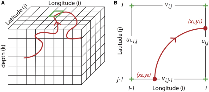
Figure 1. Principles of the combined Eulerian-Lagrangian approach. (A) Schematic of a random Lagrangian trajectory (red line) driven by the Eulerian current (u,v,w) in a three-dimensional grid model. (B) Details of the green box in (A), showing a Lagrangian computation in the horizontal plane (w = 0) (Döös et al., 2013).

On the other hand, a Lagrangian approach consists of following a water parcel or a living individual as it moves with the flow. In this ‘particle-tracking’ method, the biological changes are analyzed along discrete trajectories of passive particles that move with the flow. Compared with the biological concentration equation in an Eulerian framework (Equation 1), in the Lagrangian frame the advection term disappears and the biomass concentration evolution equation along a moving fluid parcel becomes:

$\begin{array}{cc}\frac{dC}{dt}=Diffusion+Sources-Sinks& (2)\end{array}$

For some biological applications, the particle is considered as a biotic component or a living individual, and can move relative to the water (e.g., the krill). An Individual Based Model (IBM) will accommodate these biological traits. Each individual advected by the current is constrained by its own physiological or behavioral traits (see Batchelder et al., 2002 for complete details) added to Equation (2). In the simplest case, a swimming behavior can be added to account for active migration of zooplankton (Carr et al., 2008) or fish eggs and larvae (Lett et al., 2008; Blanke et al., 2012). This active migration can be strong and reach up to several thousands of meters in the water column for some zooplanktonic taxa like Euphausiids (Brinton, 1967). Including behavior in Equation (2) helps to diagnose how individual and environmental processes combine to influence the transport of active organisms. On the other hand, understanding how the environment regulates nutrient input variability and controls phytoplankton growth does not typically require the addition of swimming behavior, and Equation (2) may be used just as is. In this case the particle is neutrally buoyant, representing an infinitesimal volume of water with movements controlled by the ambient currents.

A fully Lagrangian approach (i.e., solving the original dynamical and biogeochemical equations following Lagrangian parcels) is rarely practical: the strain and vorticity of the flow rapidly produce complex spatial distributions of the particles that form the calculation nodes. Understanding such output usually requires remapping the Lagrangian particle locations and properties to a regular grid. However, this approach has numerous drawbacks (e.g., Bailey et al., 2010).

A more fruitful approach is to use the Eulerian advective flows to create Lagrangian trajectories. Such approaches have been used in biogeochemical and ecological studies to characterize planktonic niches (Lehahn et al., 2007; D'Ovidio et al., 2010), to study how zooplankton transport is affected by mixing (Qiu et al., 2010), and to follow planktonic changes along trajectories (Abbott et al., 1990). Significantly, no such studies have aimed to identify how dynamical regional features, like mesoscale eddies or submesoscale filaments, drive the local ecosystem dynamics.

Lagrangian methods have been extensively used not only in numerical studies but also directly at sea. For example, in situ drifters were used to describe lateral advection and eddy dispersion (Davis, 1983, 1991), and the main circulation of the ocean (e.g., Owen, 1991; Richardson, 1993) or to study air-sea CO₂ fluxes (Merlivat et al., 2014), and biological processes along their path (Landry et al., 2009).

Numerical Lagrangian approaches have some distinct advantages over field deployments. First, numerical experiments can provide stronger statistical power due to the large numbers of drifters that can be deployed. Second, particles can be tracked backward in time to reconstruct the history of a water parcel. And third, in models the drifters can track vertical motions, moving in three dimensions, unlike most in situ drifters that follow only the horizontal components of the current. Present-day computational resources make it possible to obtain sufficient spatial and temporal resolution to resolve meso- and submesoscale features using Lagrangian methods. It is this aspect that we highlight with our combined Eulerian-Lagrangian approach. In particular, we apply Lagrangian analyses to the study of coherent eddies—an ideal testbed (Beron-Vera et al., 2008; D'Ovidio et al., 2013), as Lagrangian particles can quantify the coherent nature of the particular flow features they are trapped in. This combined Eulerian-Lagrangian approach allows tracking of the evolution of all the biological properties associated with a moving water parcel, in both coherent and transient structures. The combined approach is introduced in the following section (Description of the Combined Eulerian-Lagrangian Approach). The method has been applied to identify the biological transformations following a moving water parcel. More precisely, analyses have been performed in EBUS to study ecosystem dynamics along mean pathways, along individual trajectories, and in complex dynamical features such as mesoscale eddies (in Section Combined Eulerian-Lagrangian Analyses in EBUS).

Description of the Combined Eulerian-Lagrangian Approach

Principles of the Combined Method in Physical Models

The Lagrangian trajectories are computed from time- and space-dependent Eulerian velocity fields, which are simulated by an OGCM such as the Regional Ocean Model System (ROMS) (Shchepetkin and McWilliams, 2005), Massachusetts Institute of Technology general circulation model (MITgcm) (Hill and Marshall, 1995) or Nucleus for European Modeling of the Ocean (NEMO) (Madec, 2008), among others. These numerical models solve the primitive equations, i.e., the Navier-Stokes equations, under the assumptions of Boussinesq and hydrostaticity, in an Eulerian grid framework—that is, at fixed points in space (Figure 1A).

The Lagrangian trajectories can be computed online, i.e., concurrently with the Eulerian run, or offline using archived Eulerian velocity fields. The latter strategy, initiated by Döös (1995) and Blanke and Raynaud (1997), is often preferable because it enables the calculation of more trajectories, without the need for strict assumptions about the distribution of the initial particle locations. Multiple offline computations require much less CPU time than online calculations because the OGCM does not need to be run every time. Finally, unlike online calculations, offline computations allow tracking the particle backward in time. However, offline computations are highly dependent on the archiving frequency of the OGCM results. This frequency needs to be settled depending on the grid resolution and scientific goals.

The Lagrangian computation is based on the trajectory equation, solved at successive positions:

$\begin{array}{cc}\frac{d{\overrightarrow{x}}_p}{dt}=\overrightarrow{v}\left({\overrightarrow{x}}_p,t\right)& (3)\end{array}$

where ${\overrightarrow{x}}_p$ is the location of particle p, $\overrightarrow{v}$ is the local velocity field with (u, v) components in a two-dimensional field [or (u, v, w) components in a three-dimensional field] (Figure 1B). Several Lagrangian tools have been developed, for example Ariane (Blanke and Raynaud, 1997), Tracmass (Döös et al., 2013), or Roff (Carr et al., 2008). We focus here on Ariane for which the assumption of mass conservation, i.e., the non-divergence of the velocity field, enables the robust tracking of particles in a three-dimensional velocity field.

Two types of Lagrangian analyses can be run with a tool such as Ariane: qualitative analyses allow the description of full trajectory details whereas quantitative analyses give average pathways within a region of interest. The former consists of the computation of individual trajectories from initial positions of particles that can be deployed anytime and anywhere within the Eulerian grid, over the whole domain or over selected smaller sub-domains (Figure 1A). At each time step of the Lagrangian integration, the position of the particles and the associated physical properties (position, salinity, temperature and depths) are recorded. Ideally, the number of particles does not exceed several thousand so they can be treated individually; this must be optimized depending on the study and computational hardware. Quantitative experiments are a generalization of qualitative experiments and consist of deploying up to several millions of particles along a control section in a predefined subdomain, during a given period (usually several weeks to several years). The experiment ends when most particles have exited the subdomain. Additional diagnostics can be performed along each trajectory computation, by testing a criterion at each time step. This criterion can be the time of integration or a spatial constraint defined by a threshold of physical properties. When the criterion is met, the particle's trajectory is stopped. The movement of a water mass, defined by the particles that compose it, can then be studied using the trajectories of these particles (Blanke and Raynaud, 1997; Blanke et al., 1999), and the physical properties can be recovered along the trajectories. From a physical point of view, quantitative experiments help determine the Lagrangian stream function and mean circulation in a specific oceanic region. In both types of experiments, the particles can be followed forward or backward in time. The latter technique is useful for tracing the origins of a given water mass.

In the real ocean, small-scale movements associated with turbulent diffusion can alter the particle motions. Lagrangian methods can account for this diffusion using a random walk algorithm that adds a stochastic component to the deterministic part of the flow. This random walk approach has also been used to simulate the biological behavior of individual organisms (e.g., Sakai, 1973) or organism aggregation (Yamazaki and Haury, 1993). However, this approach introduces a supplementary degree of complexity. In “pure advective methods” as in Ariane, the advection term is dominant and this small-scale turbulent diffusion is ignored. In this case, only the deterministic velocity components from the OGCM are used to calculate the trajectories. This is a common approach (e.g., Chen et al., 2003; Pous et al., 2010; Auger et al., 2015) and we recognize its limitation. However, OGCMs include such turbulent mixing as a subgridscale diffusivity, thus its signature is present in the physical and biogeochemical properties interpolated along the Lagrangian trajectories. Moreover, if diffusion were included in the movements using a random walk algorithm, one should be very reserved about the interpolation of backward integrations to trace the history of water parcels because of the irreversibility of the diffusion process. Note that the computed trajectories might vary depending on the archiving frequency; with a higher frequency, trajectories more accurately follow fine-scale structures. Accounting for fine-scale structures in the Eulerian framework, the variations of physical tracers along the corresponding Lagrangian trajectories are thus related to the lateral and vertical turbulent mixing processes that are deliberately ignored in the calculation of the particle motions.

Extension of the Combined Method for Analysis of Plankton Dynamics

Our present focus on the first trophic level, exclusively composed of passive planktonic organisms whose dynamics are mainly constrained by advection, allows us to use the Lagrangian approach as a “pure advective model”. Such an approach has been used for decades and, as detailed in Section Modeling Biological-physical Interactions, numerous trajectory models have been developed, often focusing on the transport of planktonic organisms such as zooplankton (Qiu et al., 2010), fish eggs or fish larvae (Lett et al., 2007; Pous et al., 2010; Blanke et al., 2012) and more recently on jellyfish (Berline et al., 2013) or young turtles (Gaspar et al., 2012).

Note that the temporal and spatial scales associated with physical and biogeochemical/ecological processes are different: most physical processes involved in these transport studies vary over weeks to months, while biological processes can fluctuate at scales less than a day. These differences in scale imply that the Lagrangian tools used until now with relatively coarse resolution OGCMs were not well suited for planktonic marine ecology—and in particular the study of the first trophic level. However, recent advances in numerical methods allowing higher temporal and spatial resolution of the OCGMs have enabled the modeling of physical processes at scales that match those of the biological processes.

The diffusion terms in Equation (2) are neglected in our Lagrangian approach under the assumption that they are much smaller than the biological terms. This simplifies the interpretation of biological variations along the trajectories: the variations experienced by biogeochemical tracers are driven only by biological processes. Diagnostics of a given tracer, including biological stock and fluxes, can be performed along the Lagrangian trajectories ${\overrightarrow{x}}_p$: quantitative experiments help to assess planktonic dynamics along the main circulation pathways at regional scales (applied in Section Biological Transformations along Regional-scale Pathways), while qualitative experiments help to assess the biological transformations along specific trajectories (in Section Biological Transformations along Individual Trajectories).

Combine Method to Follow Mesoscale Features and associated Biological Processes

The basic principles through which mesoscale eddies act on oceanic tracers are well understood (Bleck et al., 1988; Gent and McWilliams, 1990; Lee et al., 1997). However, their roles in ecosystem dynamics have not been fully described and explained despite continued interest in the effects of mesoscale turbulence on biogeochemical activity (Gower et al., 1980; Jenkins, 1988; McGillicuddy et al., 1998, 1999, 2001; Lévy, 2008; Klein and Lapeyre, 2009) and numerous available observations (e.g., Nencioli et al., 2008). In particular, because the overall effect of mesoscale turbulence is a mixture of advective and diffusive processes, it is difficult to delimit the boundaries of eddies and assess the associated biophysical dynamics. We used the Lagrangian approach to follow numerical particles trapped in eddies that were coherent and quasi-axisymmetric, and analyze the biological processes occurring in these features.

Multiple techniques have been used to detect and delimit eddy boundaries; the most common can be merged into two categories. The first method is based on physical fields such as the Sea Surface Height (SSH) anomaly (Henson and Thomas, 2008; Chaigneau et al., 2009; Chelton et al., 2011), the vorticity (McWilliams et al., 1999), the velocity gradient tensor or Okubo-Weiss (OW) parameter (Isern-Fontanet et al., 2003, 2004; Morrow et al., 2004; Chelton et al., 2007; Sangrà et al., 2009). The second method detects the curvature or the shape of instantaneous streamlines, assuming that eddies evolve as quasi-circular flow patterns. These geometrical approaches include the winding-angle method (Sadarjoen and Post, 2000), vector geometry (Nencioli et al., 2010), wavelets (Luo and Jameson, 2002; Doglioli et al., 2007; Sangrà et al., 2009) or Lagrangian coherent structures (Beron-Vera et al., 2008). The SSH anomaly and OW criteria remain the most popular approaches. There is no acknowledged best method and both categories have their limitations. For example, a physical-based method often requires the definition of a threshold to determine the boundaries of the eddy: small variations of this threshold can significantly change its geometry (Souza et al., 2011). Disadvantages of the geometric method include the possible inclusion of filaments surrounding the eddy (with the wavelet methods) and substantial computational costs (with the winding-angle method). Sometimes, these techniques are combined to allow for better eddy detection, tracking and delimitation (e.g., Nencioli et al., 2010).

Here, we propose a method to define boundaries within mesoscale structures through qualitative experiments using the Lagrangian approach by defining specific areas based on particle positions and properties. Particles that are trapped within eddies and transported together can be used to define the extent of relevant areas in relation to the moving coherent structure. These areas—dynamical boxes—are used to compute diagnostics of the biological and physical processes calculated from the Eulerian model. The details of this combined Eulerian-Lagrangian method are developed in Section Biological Transformations in Dynamical Boxes.

Combined Eulerian-Lagrangian Analyses in EBUS

An Introduction to EBUS

In this section, we present various applications of (1) the extended Lagrangian approach to get biogeochemical variations along trajectories and (2) the Eulerian-Lagrangian approach to study planktonic ecosystem dynamics. The examples presented here focus mainly on two of the four major EBUS: the Benguela Current upwelling system located along the southwest coast of Africa (Figure 2A, and Section Biological Transformations along Regional-scale Pathways, and Section Biological Transformations along Individual Trajectories: A Case Study and the Importance of the Eulerian Output Frequency), and the California Current upwelling system along the U.S. west coast (Figure 2B, and Section Biological Transformations along Individual Trajectories: A Case study to Assess Biology along Trajectories, and Section Biological Transformations in Dynamical Boxes).

FIGURE 2

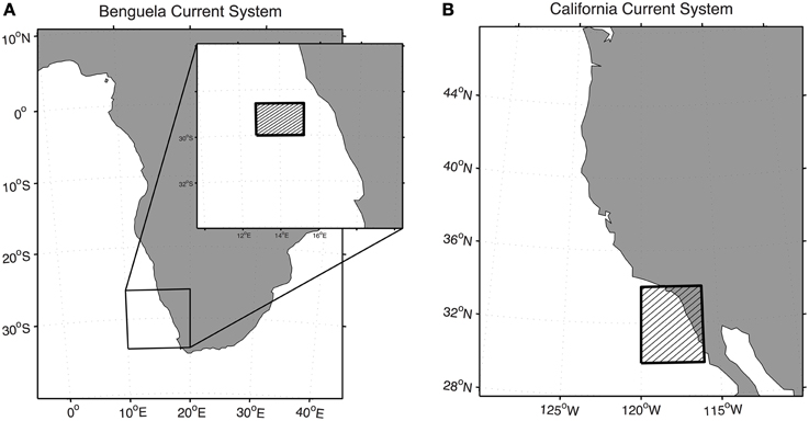
Figure 2. Regions of study. (A) The Benguela Current upwelling system located along the southwest coast of Africa and (B) the California Current upwelling system along the U.S. west coast. For each region, the studies focused on the shaded area.

EBUS provide numerous unresolved questions concerning biophysical interactions. EBUS are characterized by strong along-shore seasonal winds that create a depression of the sea surface along the coast. This depression is compensated by an intense upwelling of deep, cold, salty and nutrient-rich water. This fertilization leads to sustained biological activity of the planktonic system and higher trophic levels. Enhanced biological activity, concentrated at the coast or nearshore, contrasts with offshore oligotrophic (i.e., nutrient-poor, low-productivity) conditions. The resulting cross-shore gradient is influenced by export of coastal material to the offshore region. This export is characterized by high variability induced by wind-driven Ekman transport and mesoscale eddy activity (Combes et al., 2013), as well as submesoscale processes including downward subduction in filaments (Ramp et al., 1991; Lathuilière et al., 2010).

EBUS regimes show pronounced lateral gradients in their physical and biogeochemical ocean components. Therefore, they represent excellent systems for exploring the role of physical processes on planktonic ecosystem dynamics using the combined Eulerian-Lagrangian approach. We introduce quantitative experiments to study large-scale processes (in Section Biological Transformations along Regional-scale Pathways), then we present qualitative experiments to follow biological transformations along specific trajectories (in Section Biological Transformations along Individual Trajectories), and within dynamical boxes (in Section Biological Transformations in Dynamical Boxes).

Biological Transformations Along Regional-scale Pathways

We address the use of the combined Eulerian-Lagrangian approach in a biophysical interaction study first using quantitative experiments. Here, we aim to trace biogeochemical properties in relation to the dominant circulation. The ROMS hydrodynamic model was configured for the Benguela Current upwelling system with 8 km horizontal resolution. The ecosystem model is a simple NPZD model that was previously used in this region (Koné et al., 2005). The Eulerian model output consists of two calendar years, archived daily. To study the across-shore transport of biogeochemical components and evolution of the properties of nearshore water masses after leaving the coastal region, Lagrangian experiments were performed over a sub-domain that covers the continental slope (Figure 2A). Lagrangian particles were deployed along a section close to the coastline (the control section) over 360 days. They were intercepted along an offshore section parallel to the control section after a maximum duration of 360 days (Figure 3).

FIGURE 3

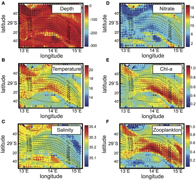
Figure 3. Results from a quantitative experiment in the Benguela Current upwelling system (Figure 2A). Vertical averages of (A) depth (m), (B) temperature (°C), (C) salinity, (D) nitrate concentration (mmolN m⁻³), (E) chlorophyll-a concentration (mg Chl-a m⁻³) and (F) zooplankton concentration (mmolN m⁻³), calculated along trajectories of the particles that traveled offshore, from the right to the left in this longitudinal section. The corresponding mean Lagrangian stream function is superimposed (black dashed contours) with a 0.01 Sv interval.

The average cross-shore pathways taken by the nearshore particles are given by the Lagrangian stream function (Figure 3). The associated transport reaches ~0.1 Sv. This dominant connection occurs in the surface layers (i.e., the upper 100 m), with a significant cross-shore transport of fresh and warm water compared to the surrounding water masses (Figures 3A–C), which is associated with many eddies traveling offshore (not shown). Because the dominant pathway occurs within the euphotic layer, i.e., the illuminated part of the water column where primary production—the basis of biological activity—occurs, interesting results concerning biological tracers might be expected. Moreover eddies associated with this main pathway are likely to trap and transport biological material from the coast (Chenillat et al., submitted ms. a,b). Indeed, compared to surrounding waters, along this pathway both the nutrient and planktonic concentrations seem to be affected: (i) the nutrient concentration is lower, because it is likely consumed by the phytoplankton; (ii) both chlorophyll-a (a proxy for phytoplankton concentration) and zooplankton biomasses are higher (Figures 3D–F). Thus, this Eulerian-Lagrangian approach has allowed us to explain and quantify the changes of nearshore planktonic organisms in relation to the physical cross-shore transport, at a regional scale. This cross-shore transport seems here to be driven by mesoscale activity; unfortunately, these analyses are insufficient to clarify the effect of this mesoscale activity on ecosystem dynamics.

In the context of biophysical interaction studies, this approach has many potential applications. For example, in regions with strong biogeochemical or physical gradients, quantitative experiments allow assessment of the transport, and the redistribution and associated changes of biological components. Large gradients of biogeochemical and physical components may develop along strong currents, along the coastline or in the cross-shore direction, or between two or more basins. Eulerian-Lagrangian diagnostics can help us understand (i) how physical properties maintain these large gradients, (ii) the exchanges among oceanic biogeographical provinces, and (iii) at finer scale, the effects of runoff on nearshore and coastal ecosystems.

A consideration of time scales is essential in such offline studies: the frequency of the available Eulerian outputs can significantly affect the results. The influence of this frequency on the biogeochemical inferences from the Lagrangian experiments is tested in the following section (Biological Transformations along Individual Trajectories).

Biological Transformations along Individual Trajectories

A Case Study and the Importance of the Eulerian Output Frequency

We performed qualitative experiments with the Lagrangian approach to find the values of biogeochemical tracers along particle paths. The trajectory of one particular particle is shown in Figure 4A, with the same Eulerian output used in Section Biological Transformations along Regional-scale Pathways. This particle was selected from among many other particles initially released along the nearshore section at around 30 m depth (see Figure 3). The trajectory shows several loops as the particle moves offshore (Figure 4A), indicating that it was trapped in an eddy. Within the eddy, the particle was upwelled to the surface, experiencing an increase in temperature of ~3°C and changes in the local biogeochemistry (not shown). This experiment clearly shows that a qualitative experiment—calculated from daily Eulerian velocity output—enables tracking of particles trapped in a mesoscale eddy. However, along-trajectory variations of biogeochemical properties could be sensitive to the frequency of the Eulerian output, leading to uncertainties on their interpretation. We thus set up specific diagnostics to study the impact of the frequency of the Eulerian output on the Lagrangian biogeochemical results.

FIGURE 4

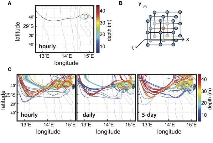
Figure 4. Results from qualitative experiments in the Benguela Current upwelling system (Figure 2A). (A) Trajectory of one reference particle that was temporarily trapped in a mesoscale eddy, calculated with hourly Eulerian outputs; its initial position is shown by the red dot. (B) Seeding strategy (2-dimensional in space and 1-dimensional in time) in the immediate neighborhood of the initial position (the red dot). (C) Trajectories of the particles initialized around the reference initial position for several sampling frequencies of the Eulerian model output: hourly (left), daily (middle), and 5-day (right). In (A,C) the color bar shows depth (in m) along trajectories.

The more frequent the Eulerian output and the higher the grid resolution, the more accurate the resolution of small-scale features in the Lagrangian trajectories. Moreover, the ecosystem processes occur at high frequency, i.e., at scales shorter than a day, which is modeled through a suitable parameterization in the Eulerian framework. Because data storage is an issue for modelers, it is essential to estimate the optimal output frequency: it must be fast enough to capture biological transformations, but coarse enough to generate a manageable amount of data. The Eulerian output frequency influences the results obtained in the offline combined Eulerian-Lagrangian approach, as shown below through a study that compared several frequencies for the same Eulerian model.

The purpose of this analysis is to compare different archiving intervals: hourly, daily and every 5 days. We chose the hourly output as a reference for the Lagrangian computations because it is fully compatible with the time scales of the biological processes and is close to the best achievable given the Eulerian model time step, usually of around 500–1000 s. The daily and 5-day archiving outputs are obtained by degrading the hourly output with a simple arithmetic average. Our diagnostics were performed on a population of particles initialized around the selected particle (Figure 4A) using a seeding strategy that consisted of duplicating the initial position in its closest neighborhood in time (t₀) and space (x₀, y₀, z₀) (as illustrated in Figure 4B). A total of 21³ (9261) particles were released. Only a few trajectories are represented in Figure 4C for the three different output intervals. This shows that despite the use of the same initial conditions, some trajectories and associated properties differ depending on the interval. These differences can be highlighted by comparing the tracer values when the particles reach the offshore section (Figure 5). We chose to explore a physically conservative tracer—salinity, and a non-conservative biological tracer—chlorophyll-a. The results obtained at hourly intervals are used as the reference (Figures 5A,C). The more the results at daily intervals and 5-day intervals differ from the reference, the less accurate they are. Cumulative histograms (Figures 5B,D) are useful for comparing the individual distributions to evaluate the effects of sampling interval. The following index estimates the differences between the test and reference distributions by integrating the square of the area of the difference between the corresponding cumulative histograms:

$\begin{array}{cc}A=\frac{{{\displaystyle {\sum }_{i=1}^N\left(Tref\left(i\right)-T(i)\right)}}^2\Delta T}{{\displaystyle {\sum }_{i=1}^N{\left(Tref(i)\right)}^2}}& (4)\end{array}$

where T is the physical or biogeochemical property tested (i.e., from either the daily or 5-day experiment), Tref is the value of reference (calculated from the hourly experiment), N is the total number of classes of the histogram, and ΔT is the class size of the histogram. ΔT is chosen to account for a total of 100 classes, and thus A represents a percentage of area difference. The 5-day output histograms are strikingly different from the hourly output histograms for both physical (A~66%) and biogeochemical tracers (~39%). This shows that 5-day output is far too coarse to reproduce accurate biophysical interactions. At the daily scale, the sensitivity to the Eulerian sampling is more marked for biogeochemical tracers (A~26%) than for physical tracers (~3%). This sensitivity to hourly vs. daily archive resolution is explained by the rapidity of biological processes: the induced non-linearities must be sampled at a suitable frequency from the Eulerian archive to ensure the quality of the Lagrangian diagnostics. It is important to note that biophysical processes can occur at time scales shorter than a day or a hour. For example, internal gravity waves can rapidly impact vertical nutrient fluxes (Wang et al., 2007). Eulerian regional models are just starting to resolve such super-inertial dynamics (e.g., Alford et al., 2015). To explicitly account for these processes in the Lagrangian model, one would need output at intervals of a few minutes. At present this would place a heavy burden on data storage, though it will become increasingly feasible in the future.

FIGURE 5

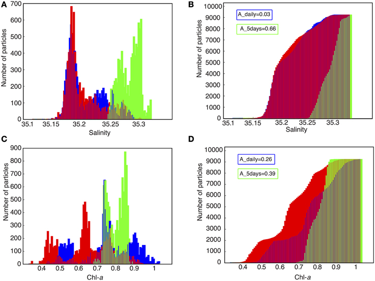
Figure 5. Effect of various Eulerian archiving intervals on Lagrangian qualitative experiments. Histograms (A–C) and cumulative histograms (B–D) of some properties of the particles initialized in the immediate neighborhood of the reference particle (see Figure 3), after trajectory calculations using hourly (red), daily (blue), and 5-day (green) subsampling frequencies of the Eulerian model output. The properties are salinity (A,B) and chlorophyll-a concentration (C,D).

Combined Eulerian-Lagrangian methods clearly need to be used with caution when analyzing biogeochemical fields from Eulerian models. The optimal archive strategy is likely the highest frequency that allows sampling of the fastest non-linear biogeochemical processes while maintaining reasonable data storage costs. In the present study, with an eddy-resolving model of ~5 km horizontal resolution, we chose a daily archive to conduct the biophysical analyses. Note that storage constraints may be somewhat lessened by aggregating horizontal grid point information as explored for offline Eulerian tracer experiments by Lévy et al. (2012).

A Case Study to Assess Biology along Trajectories

Qualitative experiments allow not only assessment of properties along individual trajectories but also visualization of the complete story of parcels of water. We present here a study that follows water trapped in a mesoscale eddy in the California Current system (Chenillat et al., submitted ms. a,b). In this numerical experiment, ROMS was coupled with an NPZD model (with several nutrient, phytoplankton, and zooplankton boxes) to study one particular cyclonic (counterclockwise) eddy evolving in the Southern California Bight (SCB) to understand how dynamical and biological processes were able to maintain biological activity within such a mesoscale feature. They chose an eddy formed at the coast that trapped and transported some nearshore water and its associated coastal upwelling ecosystem offshore.

The combined Eulerian-Lagrangian approach (Figure 6) was implemented as follows: a 2-year-long simulation was run with the Eulerian model (the first and the second year are noted Y1 and Y2, respectively) with daily output. A cyclonic eddy was chosen from this simulation based on a local minimum of the SSH (see Figure 7C) and locally enhanced biological activity. Over 7 months, this eddy traveled from the coast to the offshore region (Figure 7). From the daily archive of this 2-year-long simulation, several sets of qualitative Lagrangian experiments were performed to follow the eddy, as detailed in Chenillat et al. (submitted ms. a) (Figure 6). In a pre-experiment ~500 particles were released along the coastline (0–200 m depth), monthly from September Y1 to March Y2 (on the first day of each month). The particles were followed until 30 March Y2 when they had spread over the SCB. Only particles within the eddy (see Figure 7C) were selected for the main Lagrangian experiments. These particles were tracked backward (see Figures 7A–B) and forward (Figure 7D) in time to identify the source of the particles, and their ultimate fate.

FIGURE 6

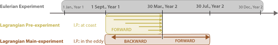
Figure 6. Schematic view of combined Eulerian-Lagrangian qualitative experiments to track a specific eddy. The gray box represents the time axis of the 2-year long (year 1 and year 2, noted Y1 and Y2, respectively) Eulerian experiment (ROMS/NPZD). The yellow and brown boxes represent two complementary Lagrangian experiments based on the Eulerian outputs. The Lagrangian pre-experiment (yellow box) consisted of releasing ~500 particles along the coastline (0–200 m depth) and monthly (from 1 September Y1 to 1 March Y2), and following them until 30 March Y2. The Lagrangian main experiment (brown box) consisted of selecting the particles present in an eddy on 30 March Y2 (see Figure 7D), and tracking them both backward and forward in time (I.P., Initial Positions).

FIGURE 7

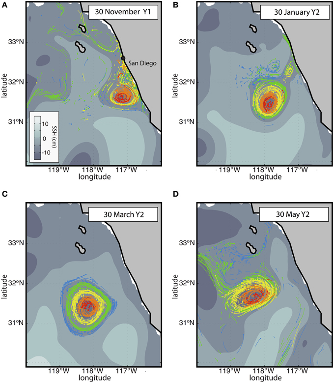
Figure 7. Time evolution of the model SSH (Eulerian outputs, in gray scale) and Lagrangian particle positions (colored dots) in an eddy of the California Current upwelling system (Figure 2B). The color code refers to different pools that were defined based on their position in the eddy on 30 March Y2, from the center (red and orange) to the edge (green and blue). The core region is defined by the red and orange particles, experiencing solid body rotation during the eddy lifetime (Chenillat et al., submitted ms. a). The trajectories during the 3 days prior to each date are drawn with thin colored lines (to keep the figure clear, only half of them are represented). The particles on display are those trapped within the eddy on 30 March Y2 (C), tracked either backward (A,B) or forward (D) in time (see Figure 6).

The gathering of physical information along the trajectories allows quantification of the kinematics of this eddy and an accurate spatial definition of the eddy's edge and core (Chenillat et al., submitted ms. a). Biological properties along these trajectories show different characteristics depending on the position of the particles within the eddy: biological activity was higher in the core than at the edge, and both regions were higher than the regional average (not shown).

Though this approach gives some insights concerning the properties in the eddy, it does not reveal the dynamics and biophysical interactions that structure the ecosystem. Additional diagnostics are thus needed and will be developed in Section Biological Transformations in Dynamical Boxes.

This combined qualitative Eulerian-Lagrangian approach to study biophysical interactions was also used by Auger et al. (2015), who released particles nearshore in a region of high cadmium (Cd) concentration, to diagnose the dispersion plume of Cd-rich water in an EBUS. They aimed to identify the source of Cd (natural or anthropogenic) that was bio-accumulating, estimated from Cd concentrations and primary production, along cross-shore trajectories.

More generally, this method can be used in marine systems to identify the origin or fate of any parcel of water, and understand any biological processes at work in the Eulerian ecosystem model. All modeled biological concentrations and fluxes can be assessed along Lagrangian trajectories, providing information about ecosystem functioning as in Auger et al. (2015). Derived properties like euphotic depth or nitracline depth can also be estimated along trajectories to define a water mass origin from biological point of view (D'Ovidio, pers. comm.). This method could provide information about water mass origins with the tracking of freshly advected nutrients from below the euphotic layer—controlling the phytoplanktonic new production—vs. “old” water that has traveled horizontally, controlling phytoplanktonic regenerated production.

Biological Transformations in Dynamical Boxes

In this last section, we highlight the role of mesoscale eddies in ecosystem dynamics by defining dynamical boxes. Mesoscale features move over time; the water linked to them can be followed using region boundaries that shift with the features: dynamical boxes. This method can help quantify and understand ecosystem evolution in such features, and assess ecosystem response to local physically driven forcing.

The dynamical box concept enhances the Lagrangian approach by providing a tool to analyze groups of particles trapped within coherent structures (see Section Biological Transformations along Individual Trajectories). The Lagrangian approach used in Chenillat et al. (submitted ms. a) showed that the cyclonic eddy was able to retain nearshore water for several months while moving offshore (Figure 7). This led to the conclusion that there was little horizontal exchange within the eddy. Nevertheless, because the particles only represent a portion of the water trapped within the eddy, they do not capture all the effects of eddies on ecosystem dynamics or the possible vertical exchanges between the euphotic zone and deeper waters: the particles trapped in the eddy tracked coastal water whereas local vertical exchanges involved non-coastal eddy waters that were not tracked in the study.

To get a complete picture of the biological responses in the eddy core, we must assess and understand ecosystem evolution in response to physically driven vertical nutrient input (Falkowski et al., 1991; McGillicuddy and Robinson, 1997). Using dynamical boxes defined according to the Lagrangian particle kinematics, Chenillat et al. (submitted ms. a) characterized the eddy core region as those particles experiencing solid body rotation during the eddy lifetime (Figure 8A). This core region changed spatially and moved over time, precluding the use of a stationary analysis region. Within this dynamical box defined by the Lagrangian particles, Eulerian diagnostics of biophysical processes showed that the core area remained relatively constant (Chenillat et al., submitted ms. a,b).

FIGURE 8

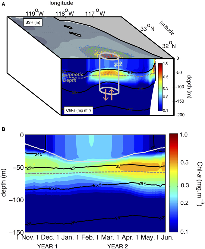
Figure 8. Biological response in an eddy of the California Current upwelling system. (A) Schematic of the dynamical box (the eddy core) defined by the red and orange pools of particles (see Figure 7C). The eddy core contains an enhanced subsurface chlorophyll-a maximum. Within this box, at each time step, vertical exchanges (orange arrows) for example across the euphotic depth can be assessed. (B) Time evolution of the total chlorophyll-a concentration averaged horizontally over the eddy core dynamical box. Superimposed on the chlorophyll-a concentration (color scale in A,B) are isolines of density (black) and euphotic depth (dashed gray line). In (B), the depth of the mixed layer is represented by the light gray line.

The Eulerian diagnostics in these dynamic boxes require horizontal averaging of the Eulerian output over the box region at each time step. Vertical exchanges such as loss of material by biological sinking (output from the eddy) or upwelling of nutrient by vertical advection (input) can then be quantified. In these dynamical boxes, any biological component represented in the ecosystem model can be diagnosed with high confidence due to the weak lateral exchanges within the box (eddy) or with the surrounding waters (Figure 8A). These components include biological concentrations (nutrients, phytoplankton, zooplankton), biological fluxes (e.g., nutrient uptake for growth, grazing, remineralization) or advective fluxes of biological components (i.e., any tracer concentrations advected by the vertical or horizontal flow). More precisely, within the dynamical box and at each time step, horizontal averages can be applied to calculate the vertical structure of any physical or biological tracer in the water column (Figure 8B). At each time step, we can also estimate the euphotic depth and evaluate any vertical exchange across this boundary, such as the nutrient input driven by advective fluxes or sinking of material (Chenillat et al., submitted ms. b).

Dynamical boxes were also defined for the waters directly surrounding the eddy. Analyses of the properties of particles in this box showed that biological activity was lower than in the eddy core, that vertical input of nutrients to the euphotic layer were low, and that horizontal exchanges were not negligible. This dynamical box method is an excellent tool for comparing processes among regions; in this case they revealed the significance of vertical nutrient input for maintaining biological activity in the eddy core compared to surrounding waters. The method can be generalized to study vertical exchanges within any coherent structure. Another interesting and fruitful application of the Eulerian-Lagrangian method combined with dynamical boxes would be to compare the dependence of the biology in eddies on the eddy properties such as their site of generation, their time of formation, their intensity, their persistence, and whether they are cyclonic or anticyclonic (see Morales et al., 2012 and references within).

Conclusions

We have developed a combined Eulerian-Lagrangian approach to study planktonic dynamics in moving fluids from numerical studies. Lagrangian approaches are particularly useful for revealing physical pathways, and the dynamics and distributions of tracers along these trajectories. A similar combined approach has been used previously in oceanography to study biological processes in response to ocean dynamics (e.g., D'Ovidio et al., 2010; Blanke et al., 2012; Berline et al., 2013); our approach provides new perspectives: it allows quantification of biogeochemical tracer dynamics both along particle trajectories, and within coherent structures—such as eddies—that are characteristic of a turbulent flow. Because physical and biological processes often occur at different frequencies, combined Eulerian-Lagrangian methods must be used with caution when analyzing biogeochemical fields from Eulerian models: the Eulerian output frequency will influence the results obtained from the offline combined Eulerian-Lagrangian approach. We showed that the optimal archive strategy balances the highest frequency that allows sampling of the fastest non-linear biogeochemical processes while maintaining reasonable data storage costs: it must be fast enough to capture biological transformations, but coarse enough to generate a manageable amount of data.

The application of this approach was focused on the planktonic ecosystem response in eastern boundary upwelling systems, where ocean dynamics drive export of coastal material offshore through intense cross-shore transport events in coherent structures. This method can be widely used to quantify any tracer dynamics in moving fluids. The code for the combined Eulerian-Lagrangian method is available upon request (Ariane-Tracer); we will use it in future work to assess the origin and age of water forming a frontal structure. In general, this method can be used to quantify any tracer dynamics, biotic or abiotic, evolving in any moving fluid or in a non-homogenous environment.

Conflict of Interest Statement

The authors declare that the research was conducted in the absence of any commercial or financial relationships that could be construed as a potential conflict of interest.

Acknowledgments

Support for this study has been provided by CNES (Centre National d'Études Spatiales), as part of the Ifesta-Up project funded by the TOSCA (Terre, Ocean, Surfaces Continentales, Atmosphère) program and by National Science Foundation (NSF) funding (OCE-10-26607) to the CCE-LTER site.

References

Abbott, M. R., Brink, K. H., Booth, C. R., Blasco, D., Codispoti, L. A., Niiler, P. P., et al. (1990). Topography san syntactic foam. J. Geophys. Res. 95, 9393–9409. doi: 10.1029/JC095iC06p09393

CrossRef Full Text

Alford, M. H., Peacock, T., MacKinnon, J. A., Nash, J. D., Buijsman, M. C., Centuroni, L. R., et al. (2015). The formation and fate of internal waves in the South China Sea. Nature 521, 65–69. doi: 10.1038/nature14399

PubMed Abstract | CrossRef Full Text | Google Scholar

Auger, P.-A., Machu, E., Gorgues, T., Grima, N., and Waeles, M. (2015). Comparative study of potential transfer of natural and anthropogenic cadmium to plankton communities in the North-West African upwelling. Sci. Total Environ. 505, 870–888. doi: 10.1016/j.scitotenv.2014.10.045

PubMed Abstract | CrossRef Full Text | Google Scholar

Bailey, D., Berndt, M., Kucharik, M., and Shashkov, M. (2010). Reduced-dissipation remapping of velocity in staggered arbitrary Lagrangian–Eulerian methods. J. Comput. Appl. Math. 233, 3148–3156. doi: 10.1016/j.cam.2009.09.008

CrossRef Full Text | Google Scholar

Ban, V. S., and Gilbert, S. L. (1975). The chemistry and transport phenomena of chemical vapor deposition of silicon from SiCl 4. J. Cryst. Growth. 31, 284–289. doi: 10.1016/0022-0248(75)90142-6

CrossRef Full Text | Google Scholar

Batchelder, H. P., Edwards, C. A., and Powell, T. M. (2002). Individual-based models of copepod populations in coastal upwelling regions: implications of physiologically and environmentally influenced diel vertical migration on demographic success and nearshore retention. Prog. Oceanogr. 53, 307–333. doi: 10.1016/S0079-6611(02)00035-6

CrossRef Full Text | Google Scholar

Berline, L., Zakardjian, B., Molcard, A., Ourmières, Y., and Guihou, K. (2013). Modeling jellyfish Pelagia Noctiluca transport and stranding in the ligurian Sea. Mar. Pollut. Bull. 70, 90–99. doi: 10.1016/j.marpolbul.2013.02.016

PubMed Abstract | CrossRef Full Text | Google Scholar

Beron-Vera, F. J., Olascoaga, M. J., and Goni, G. J. (2008). Oceanic mesoscale eddies as revealed by Lagrangian coherent structures. Geophys. Res. Lett. 35, L12603. doi: 10.1029/2008gl033957

CrossRef Full Text | Google Scholar

Bird, R. B., Stewart, W. E., and Lightfoot, E. N. (2007). Transport Phenomena, 2nd Edn. New York, NY: John Wilwe & Sons, Inc.

Blanke, B., Arhan, M., Madec, G., and Roche, S. (1999). Warm water paths in the equatorial Atlantic as diagnosed with a general circulation model. J. Phys. Oceanogr. 29, 2753–2768.

Google Scholar

Blanke, B., Bonhommeau, S., Grima, N., and Drillet, Y. (2012). Sensitivity of advective transfer times across the North Atlantic Ocean to the temporal and spatial resolution of model velocity data: implication for European eel larval transport. Dyn. Atmos. Oceans. 55–56, 22–44. doi: 10.1016/j.dynatmoce.2012.04.003

CrossRef Full Text | Google Scholar

Blanke, B., and Raynaud, S. (1997). Kinematics of the pacific equatorial undercurrent: an eulerian and lagrangian approach from GCM results. Oceanogr. J. Physical. 27, 1038–1053.

Google Scholar

Bleck, R., Onken, R., and Woods, J. D. (1988). A two-dimensional model of mesoscale frontogenesis in the ocean. Q. J. R. Meteorol. Soc. 114, 347–371. doi: 10.1002/qj.49711448005

CrossRef Full Text

Brinton, E. (1967). Distributional atlas of Euphausiacea (Crustacea) in the California current region. Calif. Coop. Oceanic Fish. Invest. 5:275.

Carr, S. D., Capet, X., McWilliams, J. C., Pennington, J. T., and Chavez, F. P. (2008). The influence of diel vertical migration on zooplankton transport and recruitment in an upwelling region: estimates from a coupled behavioral-physical model. Fish. Oceanogr. 17, 1–15. doi: 10.1111/j.1365-2419.2007.00447.x

CrossRef Full Text | Google Scholar

Chai, F., Dugdale, R. C., Peng, T., Wilkerson, F. P., and Barber, R. T. (2002). One-dimensional ecosystem model of the equatorial pacific upwelling system. Part I: model development and silicon and nitrogen cycle. Deep Sea Res. Part II. 49, 2713–2745. doi: 10.1016/S0967-0645(02)00055-3

CrossRef Full Text | Google Scholar

Chaigneau, A., Eldin, G., and Dewitte, B. (2009). Eddy activity in the four major upwelling systems from satellite altimetry (1992–2007). Prog. Oceanogr. 83, 117–123. doi: 10.1016/j.pocean.2009.07.012

CrossRef Full Text | Google Scholar

Chelton, D. B., Schlax, M. G., and Samelson, R. M. (2011). Global observations of nonlinear mesoscale eddies. Prog. Oceanogr. 91, 167–216. doi: 10.1016/j.pocean.2011.01.002

CrossRef Full Text | Google Scholar

Chelton, D. B., Schlax, M. G., Samelson, R. M., and de Szoeke, R. A. (2007). Global observations of large oceanic eddies. Geophys. Res. Lett. 34, L15606. doi: 10.1029/2007gl030812

CrossRef Full Text | Google Scholar

Chen, C., Xu, Q., Beardsley, R. C., and Franks, P. J. S. (2003). Model study of the cross-frontal water exchange on Georges Bank: a three-dimensional Lagrangian experiment. J. Geophys. Res. 108, 3142. doi: 10.1029/2000JC000390

CrossRef Full Text | Google Scholar

Chenillat, F., Rivière, P., Capet, X., Franks, P. J. S., and Blanke, B. (2013). California coastal upwelling onset variability: cross-shore and bottom-up propagation in the planktonic ecosystem. PLoS ONE 8:e62281. doi: 10.1371/journal.pone.0062281

PubMed Abstract | CrossRef Full Text | Google Scholar

Combes, V., Chenillat, F., Di Lorenzo, E., Rivière, P., Ohman, M. D., and Bograd, S. J. (2013). Cross-shore transport variability in the California current: ekman upwelling vs. eddy dynamics. Prog. Oceanogr. 109, 78–89. doi: 10.1016/j.pocean.2012.10.001

CrossRef Full Text | Google Scholar

Davis, R. E. (1983). Oceanic property transport, lagrangian particle statistics, and their prediction. J. Mar. Res. 41, 163–194. doi: 10.1357/002224083788223018

CrossRef Full Text | Google Scholar

Davis, R. E. (1991). Observing the general circulation with floats. Deep Sea Res. Part A. 38, S531–S571. doi: 10.1016/S0198-0149(12)80023-9

CrossRef Full Text | Google Scholar

Dewan, A. (2011). Tackling Turbulent Flows in Engineering. Berlin; Heidelberg: Springer-Verlag.

Google Scholar

Doglioli, A. M., Blanke, B., Speich, S., and Lapeyre, G. (2007). Tracking coherent structures in a regional ocean model with wavelet analysis: application to cape basin eddies. J. Geophys. Res. 112, C05043. doi: 10.1029/2006JC003952

CrossRef Full Text | Google Scholar

Döös, K. (1995). Interocean exchange of water masses. J. Geophys. Res. 100, 13499–13514. doi: 10.1029/95JC00337

CrossRef Full Text | Google Scholar

Döös, K., Kjellsson, J., and Jönsson, B. (2013). “TRACMASS—a lagrangian trajectory model,” in Preventive Methods for Coastal Protection, Towards the Use of Ocean Dynamics for Pollution Control (Berlin; Heidelberg: Springer), 225–249.

D'Ovidio, F., De Monte, S., Alvain, S., Dandonneau, Y., and Lévy, M. (2010). Fluid dynamical niches of phytoplankton types. Proc. Natl. Acad. Sci. U.S.A. 107, 57–59. doi: 10.1073/pnas.1004620107

PubMed Abstract | CrossRef Full Text | Google Scholar

D'Ovidio, F., De Monte, S., Della Penna, A., Cotté, C., and Guinet, C. (2013). Ecological implications of eddy retention in the open ocean: a lagrangian approach. J. Phys. A Math. Theor. 46, 1–21. doi: 10.1088/1751-8113/46/25/254023

CrossRef Full Text | Google Scholar

Estrada, M., and Berdalet, E. (1997). Phytoplankton in a turbulent world. Sci. Mar. 61, 125–140.

Google Scholar

Falkowski, P. G., Ziemann, D., Kolber, Z., and Bienfang, P. K. (1991). Role of eddy pumping in enhancing primary production in the ocean. Nature 352, 55–58. doi: 10.1038/352055a0

CrossRef Full Text | Google Scholar

Franks, P. J. S. (2002). NPZ models of plankton dynamics: their construction, coupling to physics, and application. J. Oceanogr. 58, 379–387. doi: 10.1023/A:1015874028196

CrossRef Full Text | Google Scholar

Gaspar, P., Benson, S. R., Dutton, P. H., Réveillère, A., Jacob, G., Meetoo, C., et al. (2012). Oceanic dispersal of juvenile leatherback turtles: going beyond passive drift modeling. Mar. Ecol. Prog. Ser. 457, 265–284. doi: 10.3354/meps09689

CrossRef Full Text | Google Scholar

Gent, P. R., and McWilliams, J. C. (1990). Isopycnal mixing in ocean models. J. Oceanogr. 20, 150–155.

Gower, J. F. R., Denman, K. L., and Holyer, R. J. (1980). Phytoplankton patchiness indicates fluctuation spectrum of mesoscale oceanic structure. Nature 288, 157–159. doi: 10.1038/288157a0

CrossRef Full Text | Google Scholar

Gruber, N., Lachkar, Z., Frenzel, H., Marchesiello, P., Munnich, M., McWilliams, J. C., et al. (2011). Eddy-induced reduction of biological production in eastern boundary upwelling systems. Nat. Geosci. 4, 787–792. doi: 10.1038/ngeo1273

CrossRef Full Text | Google Scholar

Haury, L. R., McGowan, J. A., and Wiebe, P. H. (1978). “Patterns and processes in the time-space scales of plankton distributions,” in Spatial Pattern in Plankton Communities, ed J. H. Steele (New York, NY: Springer), 277–327.

Henson, S. A., and Thomas, A. C. (2008). A census of oceanic anticyclonic eddies in the Gulf of Alaska. Deep Sea Res. Part I 55, 163–176. doi: 10.1016/j.dsr.2007.11.005

CrossRef Full Text | Google Scholar

Hill, C., and Marshall, J. (1995). Application of a parallel navier-stokes model to ocean circulation in parallel computational fluid dynamics, in Proceedings of Parallel Computational Fluid Dynamics: Implementations and Results Using Parallel Computers (New York, NY: Elsevier Science B.V), 545–552.

Isern-Fontanet, J., Font, J., García-Ladona, E., Emelianov, M., Millot, C., and Taupier-Letage, I. (2004). Spatial structure of anticyclonic eddies in the algerian basin (Mediterranean Sea) analyzed using the okubo–weiss parameter. Deep Sea Res. Part II 51, 3009–3028. doi: 10.1016/j.dsr2.2004.09.013

CrossRef Full Text | Google Scholar

Isern-Fontanet, J., García-Ladona, E., and Font, J. (2003). Identification of marine eddies from altimetric maps. J. Atmos. Oceanic Technol. 1995, 772–778. doi: 10.1175/1520-0426(2003)20<772:IOMEFA>2.0.CO;2

CrossRef Full Text | Google Scholar

Jenkins, W. J. (1988). Nitrate flux into the euphotic zone near Bermuda. Nature 331, 521–523. doi: 10.1038/331521a0

CrossRef Full Text | Google Scholar

Kiørboe, T. (1993). Turbulence, phytoplankton cell size, and the structure of pelagic food webs. Adv. Mar. Biol. 29, 1–72.

Google Scholar

Klein, P., and Lapeyre, G. (2009). The oceanic vertical pump induced by mesoscale and submesoscale turbulence. Ann. Rev. Mar. Sci. 1, 351–375. doi: 10.1146/annurev.marine.010908.163704

PubMed Abstract | CrossRef Full Text | Google Scholar

Koné, V., Machu, E., Penven, P., Andersen, V., Garçon, V., Fréon, P., et al. (2005). Modeling the primary and secondary productions of the southern benguela upwelling system: a comparative study through two biogeochemical models. Glob. Biogeochem. Cycles 19:GB4021. doi: 10.1029/2004GB002427

CrossRef Full Text | Google Scholar

LaCasce, J. H. (2008). Statistics from lagrangian observations. Prog. Oceanogr. 77, 1–29. doi: 10.1016/j.pocean.2008.02.002

CrossRef Full Text | Google Scholar

Landry, M. R., Ohman, M. D., Goericke, R., Stukel, M. R., and Tsyrklevich, K. (2009). Lagrangian studies of phytoplankton growth and grazing relationships in a coastal upwelling ecosystem off Southern California. Prog. Oceanogr. 83, 208–216. doi: 10.1016/j.pocean.2009.07.026

CrossRef Full Text | Google Scholar

Lathuilière, C., Echevin, V., Lévy, M., and Madec, G. (2010). On the role of the mesoscale circulation on an idealized coastal upwelling ecosystem. J. Geophys. Res. 115, C09018. doi: 10.1029/2009JC005827

CrossRef Full Text | Google Scholar

Lee, M. M., Marshall, D. P., and Williams, R. G. (1997). On the eddy transfer of tracers: advective or diffusive? J. Mar. Res. 55, 483–505. doi: 10.1357/0022240973224346

CrossRef Full Text | Google Scholar

Lehahn, Y., D'Ovidio, F., Lévy, M., and Heifetz, E. (2007). Stirring of the Northeast Atlantic spring bloom: a lagrangian analysis based on multisatellite data. J. Geophys. Res. 112, C08005. doi: 10.1029/2006JC003927

CrossRef Full Text | Google Scholar

Lett, C., Penven, P., Ayón, P., and Fréon, P. (2007). Enrichment, concentration and retention processes in relation to anchovy (Engraulis Ringens) eggs and larvae distributions in the northern humboldt upwelling ecosystem. J. Mar. Syst. 64, 189–200. doi: 10.1016/j.jmarsys.2006.03.012

CrossRef Full Text | Google Scholar

Lett, C., Verley, P., Mullon, C., Parada, C., Brochier, T., Penven, P., et al. (2008). A lagrangian tool for modelling ichthyoplankton dynamics. Environ. Model. Softw. 23, 1210–1214. doi: 10.1016/j.envsoft.2008.02.005

CrossRef Full Text | Google Scholar

Lévy, M. (2008). “The modulation of biological production by oceanic mesoscale turbulence,” in Transport and Mixing in Geophysical Flows (Berlin; Heidelberg: Springer), 219–261.

Lévy, M., Resplandy, L., Klein, P., Capet, X., Iovino, D., and Ethé, C. (2012). Grid degradation of submesoscale resolving ocean models: benefits for offline passive tracer transport. Ocean Model. 48, 1–9. doi: 10.1016/j.ocemod.2012.02.004

CrossRef Full Text | Google Scholar

Lih, M. M. S. (1975). Transport Phenomena in Medicine and Biology (Biomedical Engineering and Health Systems), 1st Edn. New York, NY: John Wiley & Sons Inc.

Longhurst, A. R. (1995). Seasonal cycles of pelagic production and consumption. Prog. Oceanogr. 36, 77–167. doi: 10.1016/0079-6611(95)00015-1

CrossRef Full Text | Google Scholar

Luo, J., and Jameson, L. (2002). A wavelet-based technique for identifying, labeling, and tracking of ocean eddies. J. Atmos. Oceanic Technol. 19, 381–390. doi: 10.1175/1520-0426-19.3.381

CrossRef Full Text | Google Scholar

Madec, G. (2008). NEMO Ocean Engine. France, Institut Pierre-Simon Laplace (IPSL), 300. (Note du Pole de Modélisation 27)

Google Scholar

McGillicuddy, D. J., Johnson, R., Siegel, D. A., Michaels, A. F., Bates, N. R., and Knap, A. H. (1999). Mesoscale variations of biogeochemical properties in the Sargasso Sea. J. Geophys. Res. 104, 381–394. doi: 10.1029/1999jc900021

CrossRef Full Text | Google Scholar

McGillicuddy, D. J., Kosnyrev, V. K., Ryan, J. P., and Yoder, J. A. (2001). Covariation of mesoscale ocean color and sea-surface temperature patterns in the Sargasso Sea. Deep Sea Res. Part II. 48, 1823–1836. doi: 10.1016/S0967-0645(00)00164-8

CrossRef Full Text | Google Scholar

McGillicuddy, D. J., and Robinson, A. R. (1997). Eddy-induced nutrient supply and new production in the sargasso sea. Deep Sea Res. Part I. 44, 1427–1450. doi: 10.1016/S0967-0637(97)00024-1

CrossRef Full Text | Google Scholar

McGillicuddy, D. J., Robinson, A. R., Siegel, D. A., Jannasch, H. W., Johnson, R., Dickey, T. D., et al. (1998). Influence ofmesoscale eddies on newproduction in the Sargasso Sea. Nature 394, 263–266. doi: 10.1038/28367

CrossRef Full Text | Google Scholar

McWilliams, J. C., Weiss, J. B., and Yavneh, I. (1999). The vortices of homogeneous geostrophic turbulence. J. Fluid Mech. 401, 1–26. doi: 10.1017/S0022112099006382

CrossRef Full Text | Google Scholar

Merlivat, L., Boutin, J., and Antoine, D. (2014). Roles of biological and physical processes in driving seasonal air–sea CO₂ flux in the southern ocean: new insights from CARIOCA pCO₂. J. Mar. Syst. 147, 9–20. doi: 10.1016/j.jmarsys.2014.04.015

CrossRef Full Text

Morales, C. E., Hormazabal, S., Correa-Ramirez, M., Pizarro, O., Silva, N., Fernandez, C., et al. (2012). Mesoscale variability and nutrient–phytoplankton distributions off central-southern chile during the upwelling season: the influence of mesoscale eddies. Prog. Oceanogr. 104, 17–29. doi: 10.1016/j.pocean.2012.04.015

CrossRef Full Text | Google Scholar

Morrow, R., Birol, F., Griffin, D., and Sudre, J. (2004). Divergent pathways of cyclonic and anti-cyclonic ocean eddies. Geophys. Res. Lett. 31, L24311. doi: 10.1029/2004gl020974

CrossRef Full Text | Google Scholar

Nencioli, F., Dong, C., Dickey, T., Washburn, L., and McWilliams, J. C. (2010). A vector geometry–based eddy detection algorithm and its application to a high-resolution numerical model product and high-frequency radar surface velocities in the Southern California bight. J. Atmos. Oceanic Technol. 27, 564–579. doi: 10.1175/2009JTECHO725.1

CrossRef Full Text | Google Scholar

Nencioli, F., Kuwahara, V. S., Dickey, T. D., Rii, Y. M., and Bidigare, R. R. (2008). Physical dynamics and biological implications of a mesoscale eddy in the lee of Hawai'i: cyclone opal observations during E-Flux III. Deep Sea Res. Part II 55, 1252–1274. doi: 10.1016/j.dsr2.2008.02.003

CrossRef Full Text | Google Scholar

Owen, W. B. (1991). A statistical description of the mean circulation and eddy variability in the northwestern Atlantic using SOFAR floats. Prog. Oceanogr. 28, 257–303. doi: 10.1016/0079-6611(91)90010-J

CrossRef Full Text | Google Scholar

Pous, S., Feunteun, E., and Ellien, C. (2010). Investigation of tropical eel spawning area in the South-Western Indian Ocean: influence of the oceanic circulation. Prog. Oceanogr. 86, 396–413. doi: 10.1016/j.pocean.2010.06.002

CrossRef Full Text | Google Scholar

Qiu, Z. F., Doglioli, A. M., Hu, Z. Y., Marsaleix, P., and Carlotti, F. (2010). The influence of hydrodynamic processes on zooplankton transport and distributions in the North Western Mediterranean: estimates from a lagrangian model. Ecol. Modell. 221, 2816–2827. doi: 10.1016/j.ecolmodel.2010.07.025

CrossRef Full Text | Google Scholar

Ramp, S. R., Jessen, P. F., Brink, K. H., Niiler, P. P., Daggett, F. L., and Best, J. S. (1991). The physical structure of cold filaments near point Arena, California, during June 1987. J. Geophys. Res. 96, 14859–14883. doi: 10.1029/91JC01141

CrossRef Full Text | Google Scholar

Richardson, P. L. (1993). A census of eddies observed in North Atlantic SOFAR float data. Prog. Oceanogr. 31, 1–50. doi: 10.1016/0079-6611(93)90022-6

CrossRef Full Text | Google Scholar

Sadarjoen, I. A., and Post, F. H. (2000). Detection, quantification, and tracking of vortices using streamline geometry. Comput. Graph. 24, 333–341. doi: 10.1016/S0097-8493(00)00029-7

CrossRef Full Text | Google Scholar

Sakai, S. (1973). A model for group structure and its behavior. Biophys. Jpn. 13, 82–90. doi: 10.2142/biophys.13.82

CrossRef Full Text

Sangrà, P., Pascual, A., Rodríguez-Santana, A., Machín, F., Mason, E., McWilliams, J. C., et al. (2009). The canary eddy corridor: a major pathway for long-lived eddies in the subtropical North Atlantic. Deep Sea Res. Part I 56, 2100–2114. doi: 10.1016/j.dsr.2009.08.008

CrossRef Full Text | Google Scholar

Shchepetkin, A. F., and McWilliams, J. C. (2005). The regional oceanic modeling system (ROMS): a split-explicit, free-surface, topography-following-coordinate oceanic model. Ocean Model. 9, 347–404. doi: 10.1016/j.ocemod.2004.08.002

CrossRef Full Text | Google Scholar

Souza, J. M. A. C., de Boyer Montégut, C., and Le Traon, P. Y. (2011). Comparison between three implementations of automatic identification algorithms for the quantification and characterization of mesoscale eddies in the South Atlantic Ocean. Ocean Sci. 7, 317–334. doi: 10.5194/os-7-317-2011

CrossRef Full Text | Google Scholar

Stommel, H. (1963). Varieties of oceanographic experience. Science 139, 572–576. doi: 10.1126/science.139.3555.572

PubMed Abstract | CrossRef Full Text | Google Scholar

The Ring Group. (1981). Gulf stream cold-core rings: their physics, chemistry, and biology. Science 212, 1091–1100. doi: 10.1126/science.212.4499.1091

PubMed Abstract | CrossRef Full Text

Wang, Y. H., Dai, C. F., and Chen, Y. Y. (2007). Physical and ecological processes of internal waves on an isolated reef ecosystem in the South China Sea. Geophys. Res. Lett. 34, L18609. doi: 10.1029/2007GL030658

CrossRef Full Text | Google Scholar

Yamazaki, H., and Haury, L. R. (1993). A new lagrangian model to study animal aggregation. Ecol. Modell. 69, 99–111. doi: 10.1016/0304-3800(93)90051-S

CrossRef Full Text | Google Scholar