Adaptive submodel selection in hybrid models

1. Introduction

The case has been made for developing systems with submodels that change their representation according to their state. Vincenot et al. (2011) identify reference cases describing the major ways system dynamics models (SD) and individual-based models (IB) can be coupled. Their final case, SD–IB model swapping, is exemplified in the models described by Bobashev et al. (2007) and Gray and Wotherspoon (2012). These papers argue that we can improve on conventional hybrid models, in terms of efficiency, fidelity, model clarity, or execution speed by using an approach that allows the submodels themselves to change during a simulation. The last two papers implement simple models which demonstrate the approach, with correspondingly simple mechanisms to control transitions between different submodels.

Some authors argue that the explicit coupling of SD models and IB models may provide greater clarity and resolution in modeling (Fulton, 2010; Vincenot et al., 2011): parts of a model that are most clearly the result of aggregate processes are likely to be better suited to modeling with a SD approach. In contrast, the parts of a system where individuals have a significant influence on their neighbors (Botkin et al., 1972) are better suited to an IB approach. This argument is closely tied to the notion of model fidelity. Following DelSole and Shukla (2010), we take fidelity to be the degree to which a model's trajectory is compatible with real trajectories. If our immediate goal is to maximize the utility of the set of submodels within a model as it runs, this must include the fidelity of the system in the decision process.

Measuring or estimating execution speed and numerical error are comparatively straight-forward, but determining model fidelity is not. Models with a high degree of fidelity should produce results which are consistent with observed data from real instances of the system they model across both a wide range of starting conditions and under the influence of ad hoc perturbations, such as fires through a forested domain. Model fidelity is addressed by DelSole and Shukla (2010) in the context of seasonal forecasting models. They explore the relationship between fidelity and skill using an information-theoretic approach. They describe skill loosely as the ability to reproduce actual trajectories, and they describe fidelity as measuring the difference between the distribution of model results and the distribution of real world results. They highlight the attractiveness of mutual information and relative entropy as measures (or at least indices) of skill and fidelity, but they observe that in their domain, climate modeling, the necessary probability distributions are unknown.

The issues of fidelity and the attendant cost/benefit balance are central to the discussion in Bailey and Kemple (1992). This paper assesses the costs and benefits of three different upgrades to an existing model designed to help determine the best mix of types of radios used in a military context; their objective is to prioritize implementation of the refinements of their model. The fundamental issues they address are substantially the same as issues that influence dynamic model selection.

The paper by Yip and Marlin (2004) compares three models used for real-time optimization of a boiler network: simple linear extrapolation from the system's current state, quadratic prediction with the coefficients based on historical data and updated at every step, and a detailed process model that corresponds closely with the physical elements of the modeled system. Their conclusion correlates the fidelity of the model with its ability to control the real-time optimization of the system. They explicitly note that there are real costs associated with the increased fidelity. These costs include model development and the need for more expensive sensors. They note that increasing fidelity in the model enabled the system to adapt to changing fuel more efficiently, and that when there were frequent changes in fuel characteristics the simpler models performed poorly.

The projects described in Little et al. (2006) and Fulton et al. (2011) both used hybrid models as a means of decreasing the run-time, and increasing the fidelity of the modeled contaminant uptake in simulated organisms. This was accomplished by mixing individual-based submodels and regional population-based systems models. Gray and Wotherspoon (2012) explicitly used changes in the representation of agents to improve the execution speed of a contamination tracking model, without losing the fidelity of the individual based uptake model. In this paper, we will develop a more general strategy which may be appropriate for more complex systems.

2. Model Organization

For clarity, we will take the term niche to refer to something in the model which could be modeled in several ways: a “porpoise” niche could be filled by many instances of an individual-based model, models of pods, or a regional SD model of the porpoises. This is essentially the same as the term component in Vincenot et al. (2011). The motivation for departing from this convention arose from confusion resulting from inadvertently using component both in a technical and non-technical sense. The close analogy between the nature of a niche in an ecosystem and the nature of a component as discussed in Vincenot et al. (2011) suggested the choice of niche.

Each of the alternative ways of representing a niche can be viewed as a submodel, and the word representation will be used to reflect a particular choice of submodel within a niche. An explicit instance of a submodel (such as a specific pod or an SD model) will be referred to as an agent. The configuration of the model at any moment consists of the particular set of submodels which fill the niches that comprise the model as a whole. For an adaptive hybrid model, there may be a large number of possible configurations and the selection of a “best” configuration is a complex matter.

Each agent running in a model must necessarily have data which can serve to characterize it for these assessments. This data would typically be some subset of its state variables, but the data alone may not be enough to base an assessment on: there may also be extrinsic data which play a role in a particular submodel's or agent's activity and impinges on its suitability. Then, the characterization of an agent—its state vector—is an amalgam of its own state and the state of other niches it interacts with, and it can be regarded as a point in the state space which the submodel is defined over.

A corresponding set of data characterizes a niche in the model; here, it is typically some appropriate aggregation of agent-level state variables (a biomass-by-size distribution, for example), relative rankings of the suitability of agents and alternative submodels, and indications of what extrinsic support all of the various alternatives require. This niche-level state vector provides the data needed for optimizing the configuration globally, and for managing the configuration when niche-wide effects become significant, for example, for an incipient epidemic.

Thus, there are three distinct levels of organization which may influence the considerations regarding the current configuration, and inform any decision about what may need to change, namely

1. Agent-level data need to be examined to determine how well-suited each agent is to its current state and the context provided by the agents it interacts with,

2. A niche-level assessment which compares the utility of each of its current agents within a niche with their alternative submodels, and

3. A model-wide assessment which determines whether there are cross-agent conflicts or unmet needs arising from a particular configuration.

The state vectors which form the domains of submodels and niches are loci in appropriate state spaces and can be encoded as an elements in appropriate vector spaces. The mathematical tools to manipulate these state vectors can then be applied to calculate the distances between two states, the similarity of loci which represent models or niches, or to identify trends or clusters.

2.1. Implications of Changing Configurations

At a basic level, hybrid models are designed to represent entities or processes in the real world in a way which brings more clarity, efficiency, or fidelity that may be possible with more traditional approaches. Adaptive hybrid models, implicitly acknowledge that the appropriate representation may change through time. An important consequence is that when a submodel in a niche changes, it may trigger changes in representation elsewhere in the model.

We might consider an example where an SD submodel which represents the prey for an SD based predator changes to IB submodels. It seems reasonable to expect the representation of the predator might follow suit. This may change the spatial resolution, the fineness of the “quantities” represented, and possibly the time steps associated with the predators and prey. Disparities in either of the first two are simple enough to deal with: modelers routinely use interpolation as a means of removing inappropriate edges, or generating subscale data, for example. Changes in an agent's time step can have a dramatic causal influence on the subsequent simulation.

Chivers (2009) discusses how individual-based models are sensitive to when state variables are updated. In his discussion, the issue arises as a result of when the probability of a predator–prey interaction is calculated relative to when the prey are removed from the system, though similar effects are also likely to occur in other contexts. The temporal sensitivity of submodels' interactions needs careful examination in order to construct submodels that proceed through time coherently and interact correctly.

Multi-agent models must have strategies to manage the agents as they step from the start of the simulation to its end. The simplest method is to make everything within the model use the shortest time step required. This is computationally inefficient in a heterogeneous model.

A better approach is the technique of variable speed splitting, such as in Walters and Martell (2004) and many others. (Figure 1) This approach allows models to step through time in different intervals by dividing the largest interval required into smaller steps that are more appropriate for the submodels with naturally shorter time scales. While models with uniform time steps are a trivial example of this approach, variable speed splitting is almost as simple and much more efficient. This technique can keep the subjective times of a set of agents moderately consistent, but ad hoc stepping changes would still seem to be awkward or difficult.

FIGURE 1

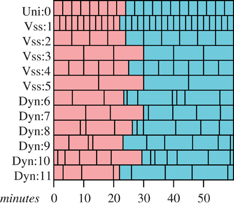
Figure 1. Time scheduling strategies. Red boxes represent time steps that have already passed, blue boxes represents scheduled time steps that have not yet been run. “Uni:” and “Vss:” submodels are members of a uniform or variable speed splitting submodels and require uniform time steps, and “Dyn:” submodels have adaptive time steps.

Both of these strategies may be subject to artifacts arising from the sequence in which agents are given their time step. The general class of model errors of the sort described in Chivers (2009) arise as a consequence of structure of the processing across the set of agents in a simulation. IB models which process agents species-by-species will be particularly vulnerable to these sorts of artifacts, since there will be an implicit advantage or disadvantage to being early in the list. Similarly, advantage or disadvantage can arise when there is a change in representation, perhaps from an SD submodel to an IB submodel; a shorter time step in this situation may introduce a great many small time steps which agents may exploit. This kind of problem can be overcome by introducing a randomizing process within each time step. Early versions of the variable speed splitting model in Lyne et al. (1994) suffered from predator–prey artifacts arising from a naïve introduction of predators and prey into the list of agents, and such randomizing was introduced to minimize the effects. In situations where the time steps of the interacting agents differ, implementing a randomization strategy may require a significant increase in the complexity of the system to accommodate irregular stepping through the lists of agents, or a significant change in the basic structure of the model.

Gray et al. (2006) and Fulton et al. (2009) describe models that have a well-developed approach to coordinating agents using adaptive time steps. In these models agents may set their own time steps to intervals that are suitable for their current activity or role. This strategy can readily incorporate submodels with uniform time steps, or collections that employ a variable speed splitting strategy. When agents interact, they either explicitly become synchronous before interaction occurs by setting their time steps appropriately and waiting, or they implicitly acknowledge that there is a temporal mismatch (Figure 1).

While some agents should be given execution priority (such as an agent which models ocean currents), most agents will have their execution order within a time step randomized, effectively preventing a large class of execution order dependent artifacts. The associated overhead in the most recent work, (Gray et al., 2006; Gray and Wotherspoon, 2012), is marginally higher than one would expect from single-stepping or variable speed stepping systems, but the advantages arising from the ability to ensure synchrony and change time steps in response to environmental stimulus outweigh the small computational overhead. This last approach seems likely to be the most appropriate for a general hybrid model that supports swapping models.

General adaptive hybrid models must have a mechanism for scheduling each agent's execution which keeps the cohort of agents roughly synchronous, and it should able to handle changes in an agent's time step when the agent changes its representation; where possible, agents should also be designed so that they may run at other time steps as well as their own preferred time step so they can become synchronous and interact at the appropriate temporal scale with other agents.

2.2. Systematically Adjusting the Model Configuration

A model's configuration should only change when there is an overall benefit in the efficiency or fidelity of the system. A straightforward way of determining this is to have a monitoring routine that runs periodically, polling the agents, and ranking likely configurations according to their relative benefit or cost. This means that each submodel would need a way to provide, to the monitor, a measure of its current suitability, and to indicate what it needs from other niches.

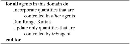
The last step in Algorithm 1 is deliberately vague.

Algorithm 1

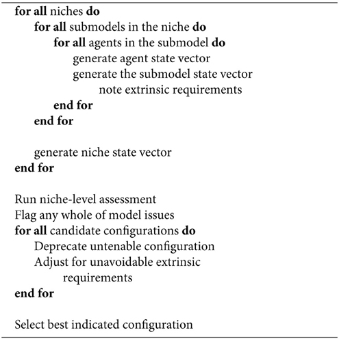
Algorithm 1. Basic processing pass for the monitor

Algorithm 1 illustrates a possible assessment pass for a monitor, though how appropriate it may be is an open question. Configuration ranking for the example model will be cast in terms of evaluating an objective function based on elements of the vector space of tree elements described in the Supplementary Material.

A monitor may have large number of potential candidate configurations, but we would like to keep the actual number quite low. The example model described below has a global domain associated with a particular representation, along with local domains (subregions of the global domain) which are associated with finer scale representations of the modeled entities. The set of potential candidate trees could be quite large; in practice we reduce the number by casting the candidate trees in a more general way—including trees representing particularly good representations and particularly poor representations: the first to steer the configuration toward good choices, and the second to drive it away from poor choices. We can use the hierarchical organization (whole-model, niche, submodel, agent) to help limit our search space, as well as the geographic context of the agents (whole-domain, local cell, immediate-locus).

The sets of candidate trees which are associated with particular configurations will need to be crafted carefully as a part of the model design. These trees reflect the modelers understanding of the strengths and weaknesses of each of the submodels (or sets of different submodels) which may be employed.

Exactly how a monitoring routine is integrated into the model framework is a subjective choice best left to the team implementing the models, but one very attractive option is to implement the monitor as an agent in the system. This would allow the monitor to assess its own performance and the needs of other agents with respect to its own suitability with the option of swapping itself for a monitor which implements some alternative strategy.

3. The Example Model

The purpose of the example model described below, is to provide a context for a discussion of the dynamics associated with a hypothetical simulation using this model. The ends of the spectrum between SD models and IB models are represented, and the environment is unrealistically simple in order to keep us from being swamped by detail.

The model consists of a spatially explicit environment that is partitioned into nine cells (Figure 2). The biotic elements consist of plants, fruit, seeds, herbivores, and carnivores. The herbivores feed on the plants and their fruit; and carnivores prey upon juvenile herbivores. The plants and herbivores are interdependent: fruit is the sole diet for juvenile herbivores and the plants need juvenile herbivores to make the seeds viable by eating the fruit.

FIGURE 2

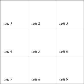
Figure 2. The model domain is divided into nine cells. An SD agent is associated with each of these cells and with the domain as a whole. Any IB agents which are created during the simulation will be associated with one cell at any given time.

The representations are equation-based SD models of the interactions between the plants and animals and IB models for plants and animals. The SD submodels model the biomass with respect to size, for plants and animals, or simply numeric quantities for fruit and seeds, and they can operate at either the global or cell-sized scale. Modeling biomass in this way makes it possible to minimize the loss of fidelity incurred by swapping from IB agents to SD agents and visa-versa, since we preserve more of the essential nature of the populations. A more detailed description of the SD agents is presented in the Supplementary Material.

Fruit and Seeds

Fruit and seeds are treated somewhat differently to the rest of the niches. They exist principally as numbers of entities that are updated as a result of the activities of other, more explicit SD or IB models. There are explicit routines that deal with uniquely “fruit” and “seed” processing to handle spoilage and germination, respectively.

For fruit and seeds we have the following relationships

$\begin{array}{l}dN\mathtt{\text{F}}(t)=Production-Spoilage-FruitEaten\end{array}$

and

$\begin{array}{l}d{N}_{\mathtt{\text{S}}}(t)=s\ast FruitEaten\hfill \\ -\left(1-\frac{N_{\mathtt{\text{P}}}(t)}{K_{\mathtt{\text{P}}}}\right)Germ.\end{array}$

where N_P(t) is the biomass of plants at time t, and K_P is the carrying capacity of the pertinent domain (either global or cell-based). The processing for fruit is quite simple and consists only of applying “spoilage”; no reference to other agents in the system is required, and only the number of fruit is adjusted as a result (Algorithm 2). Seed models will adjust their “seed count” as well as the biomass distribution for plants in their time step, according to the level of germination. Germination is probabilistic as is the size of the plant a germinated seed becomes in its pass, though the distribution of possibly sizes is quite restrained (Algorithm 3).

Algorithm 2

Algorithm 2. Basic processing pass for fruit

Algorithm 3

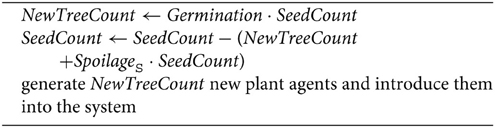
Algorithm 3. Basic processing pass for seeds

SD Representations

Each of the niches has an integral equation expressing the change in biomass for a given size; an animal's equation is of the form¹

$\begin{array}{l}d{N}_{\text{A}}(t,x)=Growth\&strave+Repr\\ -PredMort-NatMort.\end{array}$

We do not include migration terms in the SD models, since that will be addressed by the IB forms. The assumption is that the SD representation is most appropriate when population levels are moderately high, and there is adequate food; under these conditions, we will assume that the net migration associated with a domain will be close to zero.

Plants are represented by similar equations, namely

$\begin{array}{l}d{N}_{\text{P}}(t,x)=\left(1-\frac{N_{\text{P}}(t)}{K_{\text{P}}}\right)[Growth+Germ]\\ -PreMort-NatMort\end{array}$

where NP(t, x) is the biomass of plants of size x at time t.

The important state variables for the SD are, for each domain, the biomass-by-size distributions for plants, herbivores, and carnivores, and the raw numbers of fruit and viable seeds.

The system of equations described in the Supplementary Material is evaluated using a fourth order Runge–Kutta algorithm; the numbers of fruit and seeds, and both the global and cell-based biomass distributions for plants and animals are updated at the end of the calculation. The model will adjust the values in the global and cell-based models to allow data from models running with better resolution (usually more localized models) (Algorithm 4) to take precedence.

Algorithm 4

Algorithm 4. Basic processing pass for the SD models

Most of the important parameters and many of the functions associated with the life history of the modeled entities are not specified. This way we may consider possible trajectories without being tied to a particular conception or parameterization of the system.

IB Representations

Individual-based representations for plants, herbivores, and carnivores follow the pattern in Little et al. (2006); fruit and seeds are only modeled in the SD representation, though their numbers are modified by the activities of the herbivores irrespective of how those herbivores are represented.

3.1. IB Plants

Plants maintain a reference to their cell, their location, a mass, and a peak mass. If a plant's mass drops below a certain proportion (P_MΩ) of its peak mass, it dies—this provides a means for the herbivores to drive the plant population to local extinction.

We will suppose that plants grow according to a sigmoidal function with some reasonable asymptote and intermediate sharpness; fruiting occurs probabilistically as in the SD representation.

The plant agent goes through the steps in Algorithm 5 in each of its time steps. In the algorithm, Γ_P(δt, mass) is an analog of the probability of a plant growing from one size to another from the SD representation, P_Mature is the parameter that indicates the mass a plant must be before it fruits, P_Fruits is the probability of a mature plant fruiting, and P_ρ is the amount of fruit relative to the fruiting area. The routine ADDFRUIT updates the models representing fruit in the domain.

Algorithm 5

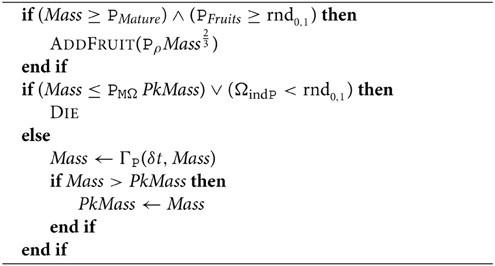
Algorithm 5. Basic processing pass for plants

3.2. IB Animals

Like the plants, animals maintain a reference to their cell, their location, and a mass. They also maintain several variables that are associated with foraging or predation, namely the amount of time until they need to eat (Sated), and the amount of time they have been hungry (Hungry).

Animals will grow while they do not need to eat and will only forage when they are hungry. Reproduction happens in a purely probabilistic way once the animal is large enough, and the young are not cared for by the parents.

Animal movement is constrained so that they will tend to stay within their nominated home cell, only migrating (changing their home cell to an adjacent cell) when food becomes scarce or if the population exceeds some nominated value and causes crowding.

The analogs of the mechanisms for growth and starvation in the SD representation are quite different to those of the IB version. In the SD models, starvation and growth occur as a result of the relative population levels of the consumer and the consumed rather than the local availability of food.

There are no real programmatic differences between the IB representations of herbivores and carnivores; their differences lie in their choices of food and the way their “time-to-eat” variable is initially managed. Individual-based, new-born carnivores begin with a long time till they need to eat. This reflects a reliance on some unmodeled foodstuff until they are large enough to prey on the juvenile herbivores. In contrast, the juvenile herbivores must begin eating fruit immediately, and only switch to foraging on plants when they are larger (but before they can reproduce). For both species, if the amount of time they have been hungry exceeds a particular value, H_Ω or C_Ω, the individual dies.

So, if we take A to represent either carnivores (C) or herbivores (H) below, then the processing pass for an animal is shown in Algorithm 6, where A_moveT is the amount of time an animal can be hungry before it migrates, A_Ω is the amount of time it takes for the animal to starve, A_EatLimit is the most the animal can eat as a proportion of its mass, A_RepSize is the minimum size an animal may breed at and A_RepP is the probability of reproducing. The routines PREYPRESENT_H and EAT_H have different cases for juvenile and adult herbivores, since juveniles prey upon fruit, and the seeds from the fruit they eat need to be accounted for in the appropriate places. There is a similar issue with juvenile carnivores. Their preylist will always be set to a value that indicates that they may eat as much as they like, and the corresponding call to EAT_C will handle this value appropriately.

Algorithm 6

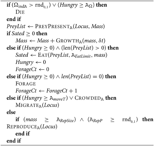
Algorithm 6. Basic processing pass for herbivores and carnivores

3.3. The Monitor and Model Dynamics

The following may be typical of the types of situations that could or should cause changes in the configuration:

• Low population—If, in an SD representation, the number of individuals filling a niche (either explicitly taken from a distribution, or estimated using a mean and a biomass) drops below a nominated value, then the biomass in that niche should be converted to IB agents representing those individuals. This type of change is motivated by the observation that at low population levels the assumption that we can treat the population as having uniform access to resources (or be uniformly available to predators) breaks down;

• High population—If a niche in a cell is represented by IB agents and the number of individuals exceeds a (higher) nominated value, the biomass those agents represent should be subsumed by the distribution in the local SD submodel. The change in representation is attractive here for two reasons: an equation-based representation will be much faster, and SD submodels are arguably simpler to calibrate;

• Starvation risk—If the mean amount of time an animal in a cell spends hungry in a cell exceeds half of A_ω (or some other nominated time), the prey biomass must convert to IB agents if it isn't already so (bearing in mind that this isn't pertinent for fruit). This mean is calculated by averaging the means of each animal in the cell. If this is triggered, it indicates that the biomass of the prey species is sparse enough that homogeneity assumption is unlikely to hold;

• Relative biomass—If the biomass available for predation is represented in a local SD agent and its density drops below some proportion of the minimum required to support the predators in the domain, the prey species should convert its biomass into IB agents and, if the predator is represented by a SD agent, it should also convert to an IB form. If the biomasses are such that the effective predation rate is unsustainable, the mixing assumption is unlikely to hold.

The pertinent data for conditions will be periodically reported to the monitor through a set of status trees. The trees are able to represent single entities, nested entities, and aggregates equally well, and can preserve structural information which may also be used in the comparison of these trees. One of the basic elements we can easily incorporate into a submodel's status tree is the agent's own assessment of its competence relative to its state-vector and its local conditions. This measure of “self-confidence” can probably be maintained at little computational cost for most agents, and may be the most significant component in a monitor's assessment. The high and low population level conditions can clearly be determined by the agent in question; it can set its level of self-confidence upward or downward as appropriate. Starvation can also be encoded in the relevant node of an agent's status tree, but since starvation alone may not indicate a problem with the way the entity is represented, it probably wouldn't reduce the value for its confidence.

A starvation trigger may usually arise as a natural consequence of the population dynamics, but it may also occur when there is a mismatch in representations which has not been adequately addressed in the design stage. The final condition based on the relative biomasses is one which properly lies in the realm of the monitor—it would be quite inefficient for each of the candidate animals to be querying their prey for available biomass, summing the result, and then noting the need for change.

The monitor will primarily use the confidence values associated with agents and their niches, and the distance from trees which describe the state of the model or its set of submodels to trees which describe “known good” configurations. With data obtained directly from the agents in the system and from alternative representations it generates status trees,

•        ${\check{\tau }}_{sn}^{\sum }$, is a candidate status tree tied to a specific configuration. The serial number, sn, ties it to a configuration with that serial number,

•        ${\check{\tau }}_d^{\sum }$, is a candidate tree which represents the current state of a domain,

         ${\tau }_t^{\sum }$, an aggregate tree for the whole domain at time t,

         ${\check{\tau }}_{sd\left(n\right),t}^{\sum }$, aggregate trees for each cell, n ∈ {1, …, 9},

         τ_{R(i), t}, specific status trees for each agent,

         τ_{R, t}, specific status trees for a representation R for each representation associated with a niche,

             and

         ${\widehat{\tau }}_{\text{R}(i),t}$, candidate trees for all possible representations of each agent i,

at the beginning of each of its steps. The model may have a mix of SD and IB representations, and some of the trees will have to incorporate data from many agents (${\tau }_t^{\sum }$, any of the ${\widehat{\tau }}_{\text{R}(i),t}$, and τ_{R, t}, for example). A candidate tree is a status tree which represents an alternative submodel in a niche, and candidate trees are generated for specific agents and for each niche. When the monitor begins to generate status or candidate trees for a given agent, it first looks to see if it has generated an appropriate tree already. If it finds one, it incorporates or adjusts the tree appropriately; perhaps by incorporating the agent's biomass and size into the tree's data. We will also denote the configuration of a domain (global or local) with ${\check{\tau }}_c^{\sum }$ where c identifies the domain in question.

The monitor assesses the trees by calculating aggregate values of particular attributes, comparing the trees' divergences from allegedly ideal configurations, and by looking how uniform groups are – groups of individuals that are all very similar are good candidates for simpler representations.

We can calculate the average confidence value from any of these trees by evaluating

$\frac{\langle \overline{\text{mask}}(\mathbf{\tau },confidence,0)\rangle }{\text{supp}(\overline{\text{mask}}(\mathbf{\tau },confidence,0))},$

for example. The trees and functions to manipulate them are described in the Appendix(Supplementary Material).

Now let us consider what a simulation might look like. Figure 3 provides an overview of the configuration of the system as our hypothetical simulation runs. The model begins with eleven agents (not counting the monitor). The monitor runs its first step generating the status trees: ${\mathbf{\tau }}_0^{\Sigma },$ which characterizes the model in aggregate, ${\mathbf{\tau }}_{SD(0),0}^{\Sigma },\dots ,{\mathbf{\tau }}_{SD(9),0}^{\Sigma },$ which record the aggregate state of the 10 SD submodels, the aggregate status tree for the IB agent, ${\mathbf{\tau }}_{IB(0),\left[9\right]}^{\Sigma }$, status trees for the SD submodels: τSD(0), 0–τSD(10), 0, the status tree for the lone carnivore, τ_{IB(11), 0}, followed by the trees which represent alternative agents: ${\widehat{\tau }}_{\text{SD}(0),0}$–${\widehat{\tau }}_{\text{SD}(10),0}$ and ${\widehat{\tau }}_{\text{IB}(11),0}$. As mentioned earlier, there is only the single tree for agent 11 (the carnivore) since its alternative representation is embodied in ${\widehat{\tau }}_{\text{SD}(10),0}$. During the simulation a simulated fire will occur.

FIGURE 3

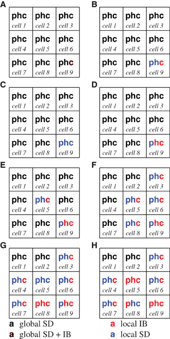
Figure 3. The color of the p,h, and c indicate an agent's current representation within a cell at various points in the description of a simulation. In each, a black symbol indicates that the biomass of plants (p), herbivores (h), or carnivores (c) is modeled with the global SD agent, a blue symbol indicates that the biomass is modeled with a cell's SD agent, and red indicates that an IB model is being used. Symbols composed of two colors indicate that more than one representation is currently controlling portions of the relevant biomass. The initial configuration of the model is represented in (A). Each of the subsequent panels (B–H) represent snapshots of the changing configuration during the simulation.

The first steps which must be taken before ranking of potential configurations is to find the sets of candidate trees which best approximate the current configuration at both the global and cell levels. We do this by calculating a similarity index or a distance which indicates how close each of the candidate trees are to the configuration of each of the domains. There are many ways we could do this: for an index which only considers structural similarity we might use something like the simple function

$\text{ssim(}c,{\tau }_d\text{)=}\frac{\text{overlap}(c,{\tau }_d)}{\max ({\Vert c\Vert }_{\text{T}},{\Vert {\tau }_d\Vert }_{\text{T}})},$

but for a more comprehensive treatment which factors values which are incorporated into the candidate and status trees we might apply the Δ(,) or dist functions described in the Supplementary Material. The dist function is a well-defined distance over the vector space of trees, while the Δ(,) function is an index of similarity that incorporates structural characteristics as well as the numerical distance between compatible subtrees. To refine such an analysis we could apply mask and $\overline{\text{mask}}$ to select only the relevant parts of the candidate and status trees.

So to assess the configuration of a domain, we would use our chosen measure to construct a set of the results of applying an optimization function, opt, to each of the candidate trees and their similarity to the current configuration. So if S is the set of all serial numbers for candidates, ${\check{\tau }}_d^{\sum }$ is the status tree fo the current domain, and, we calculate

$(C)=\{(\delta \text{(}{\check{\tau }}_d^{\sum },{\check{\tau }}_i^{\sum }),i):\forall i\in S\},$

and this is used to generate

$C^{*}=\{(\text{opt(}{\check{\tau }}_i^{\sum }),c,{\check{\tau }}_i^{\sum },i):\forall (c,i)\in C\}$

where δ stands for our chosen measure of similarity.

The elements in C* are then assessed by the monitor, and the best permissible candidate is selected. If there is only a small improvement on the current configuration, ${\check{\tau }}_d^{\sum }$, the monitor will leave the configuration as it is; otherwise, the monitor would then manage the creation of new agents to replace less optimal representations and manage the exchange of state data.

So the early phase of our simulation might begin like so:

1. Both of the aggregate trees ${\mathbf{\tau }}_0^{\Sigma }$ and ${\mathbf{\tau }}_{SD(9),0}^{\Sigma }$ indicate that there is an IB agent in their domain and that their SD representation does not perform well for the indicated biomass. Both the status and candidate trees for agent 11, τ₁₁₍₀₎,, τ_{IB(11), 0} and ${\widehat{\tau }}_{\text{IB(11),0}}$, indicate that it is confident that it can represent the biomass, and that there are no immediate unmet requirements from other agents. (Figure 3A).

2. The monitor assesses the trees against a prepared set of configurations: each of the alternative configurations (including the current configuration) is compared to a set of prepared, “efficient” configurations. The configuration of cell 9, ${\check{\tau }}_9^{\sum }$, notes global SD representations for plants and herbivores. This configuration is ranked lower than the alternative which has an individual based model for carnivores and a local SD submodel for the other entities in the cell. The monitor makes this change in configuration, and informs the global SD agent that it is no longer controlling the biomasses in cell 9 (Figure 3B).

3. The model may run for some time without any change in configuration. Both the herbivores and carnivores breed. The increased execution speed between C and D in Figure 4 is a result of a change in representation: the number of carnivores, recorded in ${\mathbf{\tau }}_{SD(C),t_4}^{\Sigma }$, reaches a point that prompts the monitor to convert them to an SD form (Figure 3C).

4. The biomass of carnivores has increased significantly by the time the model reaches D in Figure 4, and they are now eating all the young herbivores; as a result the carnivore population is now prey-limited, and the Relative biomass condition is triggered. Both the carnivore and herbivore populations are converted to IB representations. Notice that dynamics in the fidelity in Figure 4 around D arise from the collapse of the carnivore's prey, followed by the increase in fidelity after the representation change at D (Figure 3D).

5. A carnivore, agent 43, has been hungry ((Hungry ≥ A_moveT) and has migrated to the cell 5 (noted in τ_IB(43),t5). As occurred in cell 9 at step 2, the monitor converts plants and herbivores in cell 5 to a local SD representation, with IB carnivores (Figure 3E).

6. A lot of activity has occurred in this monitor interval: a Starvation risk is triggered in cell 9 because too many of the carnivores are hungry (many of the τ_IB(n)t,7 trees indicate that the elapsed time without eating is greater than Hungry). There has been more migration to cells 5,6 and 8 from cell 9 (more of the τ_IB(n),t7 trees indicate residence in new cells), and a chance migration has introduced a carnivore into cell 3 from cell 5. Cells 3,6 and 8 are converted to local SD and IB representations as happened in step 3 (Figure 3F).

7. The population of carnivores in cell 9 crashes as a result of migration and the scarcity of prey, (reported in ${\check{\tau }}_9^{\sum }$) The IB juvenile herbivores are patchy and harder to find, so only a few carnivores are getting enough to eat. There will be many τ_IB(n)t10 which indicate hunger or death due to starvation. The monitor cleans up the dead agents. There are chance migrations from cell 5 into cells 4 and 7 (in ${\mathbf{\tau }}_{SD(4),0}^{\Sigma }$ and ${\mathbf{\tau }}_{SD(7),0}^{\Sigma }$). A fire begins in cell 8, moving through cell 5: biomass loss in all niches causes all niches to shift to IB representations (Figure 3G).

8. Juvenile herbivores are reappearing in cell 9, but the available plant biomass (recorded in τSD(9), t₁₁) has dropped due to reduced germination rates, triggering the Relative biomass condition in cell 9 causing the plants to convert to an IB representation. The fire in cell 8 has killed all animal biomass in the cell; they do not return to the global SD representation because their status trees diverge by too much. Instead, they convert to local SD representations (which represent zero biomass quite efficiently). Plants remain as IB agents The fire spreads to cell 5. Figure 4 shows a modest increase in execution speed between G and H due to the population losses associate with the fire (Figure 3H).

• …the simulation continues.

FIGURE 4

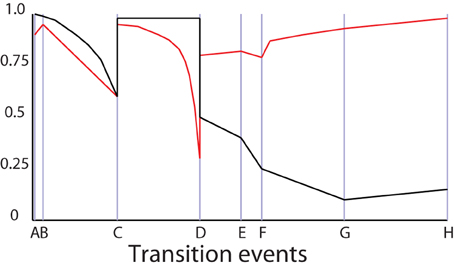
Figure 4. Normalized indexes of execution speed (black) and fidelity (red) the against configuration changes through time associated with Figure 3.

4. Discussion

Adaptive hybrid models can be constructed so that each submodel is aware of its other representations and is able to change form as appropriate (Gray and Wotherspoon, 2012). This approach requires each model to have a reasonably close coupling with its alternative representations, and the burden of instrumenting (and maintaining) the necessary code quickly becomes untenable in complex models. Worse, it removes the possibility of more subtle configuration management that can accept poor performance in one part of a system in exchange for much better performance elsewhere. It seems that a guiding principle should be that in an adaptive hybrid model, each representation should know only as much about the rest of the model as it must know, and no more. The facility for a submodel to delve into the workings of other submodels, or the workings of the model as a whole, decreases the clarity that hybrid modeling makes possible, and opens avenues for unwanted, unanticipated behavior.

The major argument in favor of closely integrated representations for submodels is that it makes common (or at least similar) state variables easy to maintain across representations, even in the face of many representation changes. It is an attractive arguement, but the long term consequence is an ever growing burden of code maintenance.

Constructing hybrid models isn't significantly more complex than constructing traditional models. Adaptive hybrid models of the sort described in this paper will require a more significant investment in the design of a monitoring routine, and in the crafting of appropriate sets of candidate configurations. The transition dynamics such a model will exhibit depend on the sets of candidate configurations, and it seems likely that a combination of analysis and experimentation may be the most effective way to develop a set of useful configurations. The hybrid models associated with (Lyne et al., 1994; Little et al., 2006; Fulton et al., 2009) were built by extending the repertoire of ways of representing elements of the ecosystem or the anthropic components rather than wholescale redesign and replacement.

We can imagine an ideal adaptive hybrid model, where any state information which must be passed on is accompanied by an appropriate, opaque parcel of code to perform the maintenance. As long as the monitor knows what information each of these maintenance interfaces needs, they can be updated each time the monitor interrogates the agent which has control of the state data. This is a readily attainable ideal: many programming languages support first class functions with closures, and these features are precisely what we need to address this problem. Scheme, Python, ML, Common Lisp, Lua, Haskell, and Scala all have first order functions with closures and, hence, the capacity to build model systems with this capability.

The state vectors and their supporting maintenance procedures can be treated as data and passed in lists associated with the status trees. If a monitor decides to swap representations, the accumulated lists of maintenance functions may be passed on to the new representation. A new representation inherits a maintenance list with variables that are part of its native state, it can claim them as its own and continue almost as though it had been running the whole time. In this way, a new representation doesn't need to know anything about its near kin, only that it must be able to run these black-box functions that come from other submodels, and to pass them on when required.

It may seem that this concentrates the global domain knowledge in the monitor, but this is not really the case. The monitor knows how to blindly query agents for state data and to the data in maintenance procedures. The monitor also knows how to recognize and rank characterizations of the states of the submodels or niches and to use those data to select a configuration.

The domain knowledge is encapsulated in the sets of targets the monitor matches the current configuration against, and in the heuristic triggers (such as Starvation risk) associated with a submodel or niche.

The essential problems any monitor is likely to deal with are problems of set selection (recognition, pattern matching…) and optimisation. These are common tasks: web searches, voice recognition, and route planning have become ingrained parts of modern society. Like route planning, the monitor needs to be able to reassess the “optimal” strategy as an ongoing process.

There are many options to choose from to rank configurations. A few of the likely candidates include

• Using an objective function to evaluate each of the possible configurations,

• Selecting a configuration based on decision trees,

• Using neural nets to match model states and direct us to an appropriate configuration,

• Using Bayesian networks to determine the most likely candidate,

and

• Using support vector machines to select the target/configuration pairs.

In writing this paper, one of the vexing difficulties has been finding a suitable mathematical representation which would allow comparisons between configurations, submodel states and the states of niches. We need proxies that describe models and configurations of models in a way that we may readily understand, manipulate and reason about, and being able to deal with submodels which are, in themselves, adaptive hybrid models, seems to be a naturally desirable trait. The vector space of trees described in the Appendix (Supplementary Material) has some nice properties, and may be directly useful with many of the options above: it forms a commutative ring (without necessarily having a unit), and would naturally inherit the body of techniques which only require the properties of such a ring.

5. Conclusion

There are still some major obstacles to developing a fully fledged adaptive hybrid model which is generic enough to tackle instances as varied as marine ecosystem modeling and urban planning. Foremost is a relative lack of real examples. The simulation of the hypothetical model² has tried to expose the character of an adaptive hybrid model which uses a monitor to manage the configuration of the system. There are parts of the description of the example system which are conspicuous by their absence; this is largely because they lie in almost wholly uncharted water. As a modeling community, we need to develop a wide range of approaches to how a model may assess the relative merits of a set of configurations. Many of the mechanisms we need for adaptive hybrid models already exist, but are found in domain specific models, and in wholly different domains, such as search engines and GPS navigation.

Establishing a suitable mathematical representation for model configurations which gives us access to well-developed techniques for set selection, pattern recognition and component analysis would seem to be almost as urgent as adaptive hybrid examples of real systems.

Conflict of Interest Statement

The authors declare that the research was conducted in the absence of any commercial or financial relationships that could be construed as a potential conflict of interest.

Acknowledgments

The authors would like to thank the two reviewers whose comments have improved the paper immeasurably. Thanks also go to a patient and understanding editor at Frontiers, and to Dr. Tony Smith, who gave up a weekend to work a scientifically and grammatically fine toothed comb through the paper. The responsibility for any mistakes, awkward sentences, or places where it just does not make sense now rests completely with the lead author.

Supplementary Material

The Supplementary Material for this article can be found online at: https://www.frontiersin.org/article/10.3389/fenvs.2015.00058

Footnotes

1. ^See the Supplementary Material for a more detailed set of equations.

2. ^The model described in this paper is currently under development and will be made freely available when it has been completed.

References

Bailey, M. P., and Kemple, W. G. (1992). “The scientific method of choosing model fidelity,” in Proceedings of the 24th Conference on Winter (New York, NY: ACM), 791–797.

Google Scholar

Bobashev, G. V., Goedecke, D. M., Yu, F., and Epstein, J. M. (2007). “A hybrid epidemic model: combining the advantages of agent-based and equation-based approaches,” in Simulation Conference, 2007 Winter (Miami, FL: IEEE), 1532–1537.

Google Scholar

Botkin, D. B., Janak, J. F., and Wallis, J. R. (1972). Some ecological consequences of a computer model of forest growth. J. Ecol. 60, 849–872. doi: 10.2307/2258570

CrossRef Full Text | Google Scholar

Chivers, W. J. (2009). Generalised, Parsimonious, Individual-based Computer Models of Ecological Systems. Newcastle, NSW: University of Newcastle.

Google Scholar

DelSole, T., and Shukla, J. (2010). Model fidelity versus skill in seasonal forecasting. J. Clim. 23, 4794–4806. doi: 10.1175/2010JCLI3164.1

CrossRef Full Text | Google Scholar

Fulton, E. (2010). Approaches to end-to-end ecosystem models. J. Mar. Syst. 81, 171–183. doi: 10.1016/j.jmarsys.2009.12.012

CrossRef Full Text | Google Scholar

Fulton, E., Gray, R., Sporcic, M., Scott, R., and Hepburn, M. (2009). “Challenges of crossing scales and drivers in modelling marine systems,” in 18th World IMACS Congress and MODSIM09 International Congress on Modelling and Simulation (Cairns, QLD), 2108–2114.

Google Scholar

Fulton, E., Gray, R., Sporcic, M., Scott, R., Little, L., Hepburn, M., et al. (2011). Ningaloo Collaboration Cluster: Adaptive Futures for Ningaloo. Technical Report 5.3, Ningaloo Collaboration Cluster, Hobart, TAS.

Gray, R., Fulton, E., Little, L., and Scott, R. (2006). Operating Model Specification Within an Agent Based Framework. North West Shelf Joint Environmental Management Study Technical Report. Number 16 in CSIRO-CMAR NWSJEMS Technical Reports. CSIRO, Hobart, TAS. doi: 10.1016/j.envsoft.2011.08.012

CrossRef Full Text

Gray, R., and Wotherspoon, S. (2012). Increasing model efficiency by dynamically changing model representations. Environ. Model. Softw. 30, 115–122. doi: 10.1016/j.envsoft.2011.08.012

CrossRef Full Text | Google Scholar

Little, L., Fulton, E., Gray, R., Hayes, D., Scott, R., McDonald, A., et al. (2006). Management Strategy Evaluation Results and Discussion for the North West Shelf. Final Report 14, CSIRO Australia, Hobart, TAS.

Lyne, V., Gray, R., Sainsbury, K., and Scott, R. (1994). Integrated Biophysical Model Investigations. Final report, CSIRO Australia, Division of Fisheries, Hobart, Tasmania.

Vincenot, C. E., Giannino, F., Rietkerk, M., Moriya, K., and Mazzoleni, S. (2011). Theoretical considerations on the combined use of system dynamics and individual-based modeling in ecology. Ecol. Modell. 222, 210–218. doi: 10.1016/j.ecolmodel.2010.09.029

CrossRef Full Text | Google Scholar

Walters, C. J., and Martell, S. J. (2004). Fisheries Ecology and Management. New Jersey: Princeton University Press.

Google Scholar

Yip, W., and Marlin, T. E. (2004). The effect of model fidelity on real-time optimization performance. Comput. Chem. Eng. 28, 267–280. doi: 10.1016/S0098-1354(03)00164-9

CrossRef Full Text | Google Scholar