Hybrid Bottom-up/Top-down Energy and Economy Outlooks: A Review of IMACLIM-S Experiments

Introduction

Bottom-up (BU) and top-down (TD) models of the energy systems have been opposed since at least Grubb et al. (1993), echoing even older distinctions dating back to the oil crises aftermath, before the revival of energy modeling prompted by the climate affair. The 2nd IPCC report highlights what is arguably the peak of the competition between the two modeling chapels (Hourcade and Shukla, 2001), after which both communities start considering bridging the gap between them through the development of hybrid models. We specifically discussed the need for such hybrid approaches in Hourcade et al. (2006). This need stems from recognizing that standard macroeconomic models, whatever their paradigm (optimal control, computable general equilibrium, econometric estimation, or the recently developing dynamic stochastic general equilibrium approach) simulate rather aggregate energy supplies and demands through mathematical functions that are (1) quite plain (for most of them continuous and infinitely differentiable), for a sheer analytical convenience that comes at the cost of maladaptation to observed or expected flexibilities of energy systems; (2) devised as first order proxies valid only in the vicinity of some initial state of the economy; (3) applied in the framework of growth theories unfit to represent technical change biased toward a drastic reduction of the energy intensity of growth. Standard macroeconomic models are thus structurally incapable of representing the major and complex technical evolutions of the energy systems, the now so-called energy transition, that the conjunction of conventional energy scarcity and the climate conundrum seems bound to induce in coming years.

Conversely, detailed energy system models offer the scope and detail necessary to capture (and aggregate at need) the complex expected evolutions of the manifold energy production techniques and end-uses;¹ but they lack the integrative macroeconomic framework necessary to evaluate the total economic costs attached to these evolutions—be it only a comprehensive description of investment markets—and thus cannot possibly account for the feedbacks between the macroeconomic constraints and the energy systems shifts.

This recognition led to develop the IMACLIM-S model as an alternative to the standard computable general equilibrium (CGE) model, focusing on providing macroeconomic consistency to the partial equilibrium results of bottom-up models. Beyond the much explored hybrid modeling strategies that link some disaggregated energy supply module to a standard CGE model, IMACLIM-S indeed constrains not only energy supply but also the energy demands of all economic agents (however aggregated) based on the explicit representation of energy systems specific to bottom-up approaches. It has done so following two quite distinct methodological avenues, which we successively present in Section Two Coupling Avenues below. In Section Data Harmonization Requirements Building Hybrid Energy/economy Accounting Tables we insist on the data harmonization necessary to a sound application of both modeling approaches of Section Two Coupling Avenues. In Section Hybrid Modeling Results we sum up various results of applied work based on either one of the two modeling methods, insisting upon the value-added of BU and TD coupling. In Section Conclusion and Further Research Agenda we draw some conclusions and reflect upon a continued research agenda.

Two Coupling Avenues

CIRED's years of research on hybrid modeling build on a profound dissatisfaction with the extension, in the wake of the 1973 oil crisis, of Solow's neoclassical growth model (Solow, 1957) to energy questions². That extension simultaneously meant:

• Applying Solow's “wrinkle” to energy, i.e., interpreting the observed energy cost shares (either aggregate or indeed sectoral) as the instantaneous results of cost minimization facing a vector of input prices.

• Generalizing the resulting production function(s) to decades of prospective outlook by simply submitting it to exogenous technical change—at first, to neutral (uniform) factor productivity improvements, as do Hudson and Jorgenson (1974); in the second wave of models spurred by the climate affair from the 1990s on, to biased productivity improvements including a specific “autonomous energy efficiency improvement” (AEEI)³.

Under such a modeling framework of energy-economy interactions, a change in energy prices at any point in time, whatever its intensity, only displaces the KLEM input mix along some pre-determined, exogenous isoquant. This cannot be a proper framework, especially in the shorter temporal terms, to assess the dramatic shifts expected from highly ambitious climate policy action, or for that matter from potential geopolitical instabilities, under the inescapable constraint of (mostly) strongly inert energy supply and end-use equipment stocks⁴.

This critique has two main implications. The first is that any relevant model of energy-economy interactions must work in an induced technical change framework, in the tradition of Kennedy (1964)—⁵, i.e., in technical terms, one that guarantees the path-dependency of substitution isoquants. To illustrate this following Ruttan (2002) (Figure 1), let us consider some time t perturbation that shifts the t+n price vector of some economy from p_t+n to p. Standard comparative statics searches the t+n impact of the perturbation on the single pre-determined production function f_t+n, thus settling on S_t+n; the point is rather to acknowledge that the perturbation induces technical change leading to a specific f production function, which induces an O′_t+n optimum. It is therefore not any unique f_t+n function but the “dynamic production frontier” F_t+n enveloping all production functions reachable from year t that should structure economic analysis⁶.

FIGURE 1

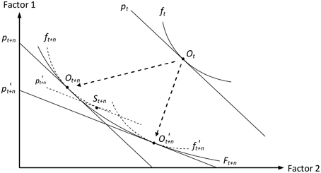
Figure 1. Induced technical change as a dynamic production frontier.

The second implication is that any macroeconomic model of energy-economy interactions is bound to turn to energy systems expertise if it is to describe with any relevance the evolution of the techniques that supply energy and convert it into service (heat, light, motion, information and communication), particularly in the short term. This has the unfortunate precondition of requiring modeling “capital” in a way closer to the physical capital actually mobilized in the processes of energy supply and demand, rather than as the ambiguous residual of value-added, labor costs subtracted, of the standard neoclassical approach.

Both implications ultimately echo the Cambridge controversy on capital, i.e., the unsettled neoclassical confusion of the economic productivity of investments for the technical efficiency of equipment⁷. Solow's own improvement of his initial model by the embodiment of technical progress in successive capital vintages (Solow, 1959) only partly addressed this critique: it introduced path-dependency but did not address the conceptual gap between flexible, continuous investment and discrete physical capital. Manne (1977) also contributed by focusing on a bottom-up representation of energy supply, thereby explicitly modeling physical capital; but he resorted to an aggregate KLE production function to project energy demand. For the same latter reason, the many subsequent CGE models that substituted some bottom-up representation of factor combinations (in varying shapes and hues) to the standard cost-minimizing energy producing sectors only partly improved on the initial KLEM model as well⁸. In the two following subsections we present our own two methods to try and overcome both identified shortcomings of the KLEM abstraction.

Calibration of Reduced Forms of Bottom-up Behaviors⁹

Our first two attempts at improving on the KLEM extension to Solow's model were literal applications of the “dynamic production frontier” interpretation of technical change. One early construction was applied work on the international climate negotiations covering 2030 projections of 14 major economies (Ghersi et al., 2003, cf. Section Reconciling the Equity and Efficiency of International Burden-sharing Climate Agreements below). A few years later, we published our improved method with illustrative projections of the global economy, also to 2030 (Ghersi and Hourcade, 2006, cf. Section The Continued Fable of the Elephant and Rabbit below). In both endeavors our bottom-up source was the POLES model of energy systems¹⁰. Focusing on climate policy, we purposely used POLES runs for a range of carbon prices broad enough to capture the “asymptotic” behavior of energy systems, i.e., the expected floor to energy intensities resulting from equipment inertia at the retained temporal horizon. To reveal our envelopes, we interpreted the results of POLES policy runs as the partial price derivatives of the static trade-off functions generated by each sequence of relative prices (Figure 2)¹¹. We did so under the notable assumption that all prices not explicitly modeled in the partial equilibrium framework of POLES, including the capital and labor prices, are constant¹².

FIGURE 2

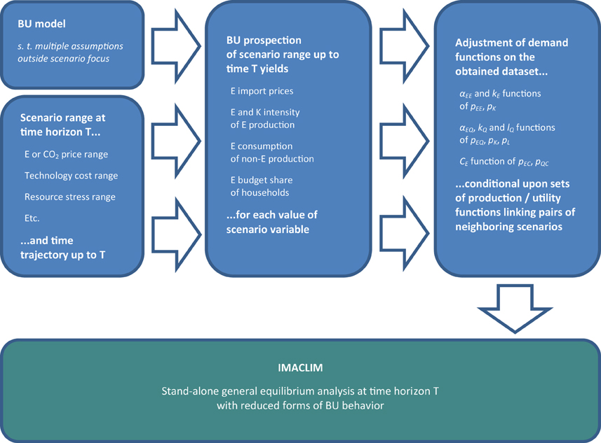
Figure 2. Calibration of reduced forms of bottom-up behaviors.

The complex practical implementation of the method and the extended geographical scope of our first experiment prompted us to focus on two-sector economies distinguishing only two goods, one energy good vs. one composite aggregate of all non-energy productions, while retaining an input-output framework easier to connect to BU expertise than value-added abstractions. In such a framework and for each economy modeled we thus required 3 “production frontiers”: one for energy production, one for non-energy production and one for households' trade-off between energy and composite goods. For the sake of concision, in what follows we only report the stabilized method thoroughly explored in Ghersi and Hourcade (2006) (Figure 2)¹³. We also do not detail the prerequisite of constructing macroeconomic tables compatible with the POLES no-policy projection to 2030 to rather focus on the method of construction of the envelopes per se at the 2030 horizon¹⁴.

Concerning energy production, for the sake of simplicity we consider that energy prices only alter the energy and capital intensities of the energy good but do not impact its labor and material intensities¹⁵. From POLES runs we draw sets of matching variations of factor intensities and prices for a range of carbon prices. Assuming constant non-energy prices allows interpreting as capital intensity shifts the variations of the monetary capital stock per physical unit of energy produced. We use the resulting dataset to calibrate the energy and capital intensities of energy production, α_EE and k_E, as functions of the ratio of their prices p_EE and p_K (Figure 2)¹⁶.

As already hinted above, a non-negligible difficulty regards identifying actual capital expenses in the cost structure of the energy sector of national accounts. The remainder of value-added (VA) net of labor costs encompasses not only capital depreciation, but also elements as heterogeneous as interest payments, rents (on land, water, mineral, and fossil resources) and a mark-up reflecting static returns to scale and/or market characteristics. Using this remainder as an index of productive equipment is therefore questionable, all the more so as the capital costs of energy supply play a key role in policy assessment. We overcome this difficulty by distinguishing, in the non-labor VA, genuine equipment expenditures, which we calibrate on total gross fixed capital formation (GFCF) data net of housing investment, and the corresponding interest payments, which we estimate thanks to a limited set of exogenous assumptions: an average capital lifespan and a real interest rate¹⁷.

Contrary to energy production, l_Q the labor content of composite (non-energy) production has a paramount influence on cost assessment, especially under imperfect labor market assumptions. We must therefore reveal a set of functions f to compute the labor content l_Q, and as a matter of fact the capital content k_Q, necessary to the calibration of the envelope of these functions. We do so assuming that:

• All policy-induced t+n economies are on a steady equilibrium path, guaranteeing to each function f the first-order conditions of relative marginal productivities equating relative prices (for any two production factors).

• For a given output and around a given energy price p_EQ, the price elasticity of energy demand is derived from POLES considering a marginal increase of p_EQ.

For a selected functional form, there is a single f making these assumptions compatible with the no-policy prices and factor-demands vectors. The same mathematical property holds successively for every pair of equilibria separated by a marginal increase of the energy or carbon price.

In Ghersi and Hourcade (2006) we assume, considering their widespread use in the E3 modeling community¹⁸, that CES functions of capital K, labor L and energy E approximate each real f at the neighborhood of the corresponding equilibrium. We calibrate CES₀ the CES prevailing at the (K₀, L₀, E₀) point of the no-policy projection by imposing (1) the linear homogeneity condition, (2) the first-order conditions at the no-policy equilibrium, and (3) the energy demand E₁ resulting from a marginally higher energy price p_EQ1 under constant other prices and output, as computed by POLES. CES₀ then yields the optimal K₁ and L₁ induced by the marginally higher price regime. We iterate this method on the newly defined (K₁, L₁, E₁) equilibrium, considering the impact of a further marginal energy price increase, as again computed by POLES. This allows the successive identification of equilibrium (K_i, L_i) compatible with POLES information on (p_EQi, E_i) couples over the whole spectrum of analysis. Note that, even though we assume a CES function at the neighborhood of each equilibrium, the resulting envelope has no reason to exhibit a constant elasticity of substitution, unless in the implausible case of a constant price elasticity of E over the range of policies explored. We use the resulting set of prices (p_EQ, p_L, p_K) and factor demands (α_EQ, l_Q, k_Q) to adjust functional forms of conditional demands of the three factors (Figure 2).

Turning to household behavior, POLES does not systematically report on the proper arguments of utility functions, i.e., energy services (heating, lighting, passenger-kilometers, etc.) whose variations may differ from those of energy consumptions per se thanks to efficiency gains. Our method consequently focuses on Marshallian demands without revealing the underlying set of utility functions. To calibrate an envelope of the Marshallian energy demand C_E, we first translate in budget share terms the changes in household energy demand computed by POLES, assuming that POLES implicitly considers constant total household expenditures¹⁹; we then adjust Marshallian demand functions by linking variations of this share to shifts of the energy and composite price, p_EC to p_QC ratio—again, considering that POLES implicitly considers constant non-energy prices.

Last but not least, we derive the impact of carbon constraints on total factor productivity in the composite sector²⁰ from a comparative-static analysis of an endogenous growth mechanism: we impact all factor intensities with a Hicks-neutral technical progress coefficient that is a function of cumulated investments. Assuming all t+n projections on a steady equilibrium path justifies using variations of the t+n equipment expenditures as a proxy of those of cumulated investment²¹. Under this specification, the crowding-out effect of mobilizing more resources in the production and consumption of energy is not accounted for through the allocation of a fixed capital stock or GFCF. Rather, firms finance their investments (equipment expenditures augmented by interest payments) under the double constraint of market balances—investment goods are produced by the composite sector—and of the ability of households' purchasing power to sustain the resulting price increases. Cumulated investments and the induced productivity of the composite sector consequently align.

Coupling Through Iterative Convergence of Linking Variables Trajectories

The ambitious “reduced form” method of Section Calibration of Reduced Forms of Bottom-up Behaviors suffers from two major drawbacks. First, its extension to a multi-sectoral framework raises conceptual issues regarding the form that the trade-off functions united by envelopes could take if further disaggregation of inputs or consumption goods were considered. Secondly, it is conditional upon the carbon pricing trajectory surmised in the bottom-up source. There is no question that simple options like a constant vs. a linearly increasing vs. an exponentially increasing tax yield contrasted “response surfaces” at the retained horizon, which implies that the calibration of reduced forms must be performed again for each specific pricing trajectory. What is more, the correspondence of BU and TD pricing trajectories is not as straightforward as it appears: the question of the reference against which the tax should be measured, i.e., the price deflator that must be applied to it to reveal its real time profile, is complex²².

For these reasons we developed a second avenue of coupling IMACLIM-S to bottom-up modeling. Rather than aiming at a standalone version of IMACLIM-S embarking bottom-up expertise (Figure 2 above), this alternative method consists in a systematic joint running of IMACLIM-S and the linked bottom-up model (Figure 3). Consistency between the two models builds on an iterative exchange of the largest possible set of shared variables or parameters, up to convergence of all elements of this set²³. More precisely, the method consists in:

• Harmonizing all the exogenous parameters common to both models, i.e., typically demography, but also possibly international energy prices, if these are exogenous to the bottom-up model as they are in the open-economy single-region versions of IMACLIM-S²⁴.

• Forcing, in the input-output framework of IMACLIM-S, bottom-up simulation results on (1) the international price of energy commodities; (2) the energy consumptions of households and the energy intensities of productions; (3) the capital intensities of energy supplies and, as far as possible, energy end-uses; (4) the volume of energy exports to foreign markets, together with that of domestic output of primary fossil energies, disaggregation permitting.

• Running IMACLIM-S under constraint of these exogenous data to compute various economic indicators (such as GDP, output at various aggregation levels but also possibly relative price variations on non-energy markets), which are sent back to the bottom-up model to serve as drivers of energy demand in a renewed simulation.

• Iterating the exchange of inputs and outputs between the two models up to convergence, in both modeling systems, of the exchanged data.

FIGURE 3

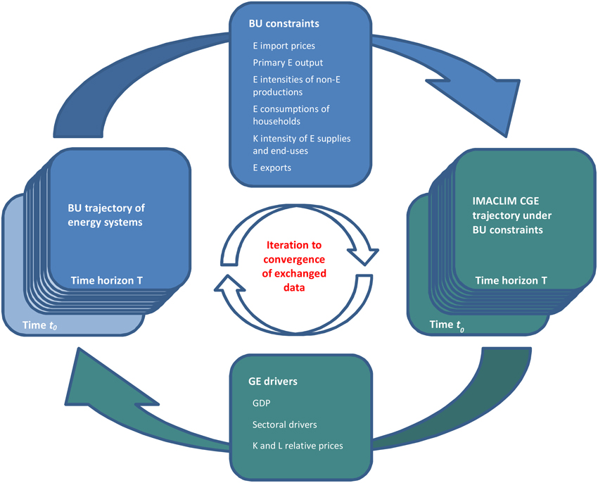
Figure 3. Coupling through iterative convergence of linking variables trajectories.

The outcome of this procedure is a consolidated set of variables consistent with both the macroeconomic framework of IMACLIM-S and the detailed energy systems modeling of the linked bottom-up model. The method naturally calls for a dynamic recursive implementation of IMACLIM-S rather than for the static comparative approach of Section Calibration of Reduced Forms of Bottom-up Behaviors: it would be pointless to feed back a deviation of GDP and other demand drivers at some unique time horizon of the initial bottom-up trajectory, while maintaining the initial trajectory up to that horizon. The exchanged data is thus in fact a set of time trajectories of the various linking variables from some common initial year (the later of the two models' starting years) to some common prospective horizon (Figure 3). Looking back at the interpretive framework of Figure 1, any envelope F_t+n now remains implicit and it is the whole path of O optima, from O_t to O_t+n, that the iterative convergence reveals—conditionally upon a parameterized context (regarding policies, technologies, resources, etc.) that changes from one run to the other.

However, contrary to the reduced form alternative the iterative method does not benefit from multiple bottom-up runs that could allow settling non-energy inputs trade-offs. One central question is again that of end-use capital, i.e., the supplemental investment in machinery, home equipment, housing insulation and transportation vehicles at the source of energy efficiency. This energy efficiency investment is increasingly explicit in bottom-up models and could eventually be fed to IMACLIM-S alongside energy demand data and energy supply capital data. Notwithstanding, the question of labor demand dynamics in non-energy sectors, together with the broader impact of relative price variations on trade-offs disconnected from energy matters, would remain unsettled. In applied work, we have thus so far resorted to conventional behavioral functions, as indeed the CES function, to settle all trade-offs but these imported from the linked bottom-up model (cf. Sections An Outlook on the Macroeconomic Impacts of Electric Vehicles Penetration in EU28 and Sovereign Risk and Energy: the RISKERGY Program below).

Concerning the behavior of producers, we thus assume that the output Y of all goods (whatever our level of disaggregation) is a function of inputs of the primary factors K and L, aggregate energy E and the composite non-energy good M²⁵, which combine in a nested structure echoing recent literature²⁶. At the bottom of the structure (Figure 4), capital K and labor L trade off to produce a KL aggregate—the capital intensity of energy production(s) is however simultaneously subject to specific productivity variations, to mirror the energy supply investment dynamics reported by the bottom-up model (cf. below). At the second tier of the input structure the KL and E aggregates combine into a KLE aggregate—which allows inferring KL intensity from the E intensity imported from BU modeling²⁷. At the third tier of the input structure, the KLE and α_M Y aggregates combine into output Y. Note that such treatment of non-energy input substitutions contradicts our induced innovation take on technical progress. We settled on it temporarily for sheer convenience, considering its widespread and well referenced use, but amending it is part of our further research agenda (cf. Section Conclusion and Further Research Agenda below). Nonetheless, the induced production frontier interpretation still holds as far as substitution between the energy bundle and value-added is concerned, thanks to the natural path-dependency of the bottom-up description of energy systems.

FIGURE 4

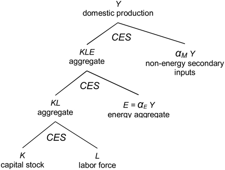
Figure 4. Nested production structure in IMACLIM-S versions iterating to convergence with BU models.

Turning to households, we directly import the volume(s) of energy consumption(s) from BU modeling and devote the remainder of the consumption budget to the composite good. In disaggregate versions, similar to production we must surmise some behavioral function to settle the competition between components of the composite good—although we will see below (Section An Outlook on the Macroeconomic Impacts of Electric Vehicles Penetration in EU28) that more than energy consumptions can be inferred from bottom-up modeling.

Regarding energy trade, which we never properly addressed in the reduced form alternative, one difficulty is that most bottom-up approaches only compute net imports as the difference between domestic output and consumption. We consequently have to disaggregate an evolution of gross exports and imports from the reported evolution of net trade²⁸. We then choose to force the resulting exports volumes and let imports balance demand. Working on major oil and gas producers (cf. Section Sovereign Risk and Energy: The RISKERGY Program) also incites us to control the price of energy exports, to reflect BU-modeled rents variations on international markets. In our approach to production, prices build up from costs—although we still consider, as we did in the reduced forms method, a fix mark-up stemming from the differentiation of capital depreciation and profits in value-added. To account for the state of international energy markets as depicted by the linked BU model, we simply adjust a specific margin (rent) on energy exports.

Similar to export prices, we want the production prices of energy to mirror variations computed in the technology-explicit framework of the linked BU model. These variations mainly reflect the capital intensification of energy supply resulting from increasingly costly conventional resources, the higher costs of the 3rd (and 4th) nuclear generation, stronger environmental constraints, the penetration of renewables, the capital requirements of “smart” distribution networks, etc. They could also reflect increased “operation and maintenance” (O&M) costs induced by shifts of the technology mix (or mixes, depending on the disaggregation of energy in IMACLIM-S), which should mean a change of the labor intensity of energy production—although the split between labor costs, materials, and indeed possible genuine capital expenses in the O&M aggregate attached to BU technologies is generally unknown.

Considering the minor share of O&M expenses in total energy costs, in applied work so far we translate all energy costs variations in capital intensity shifts. To do so we develop an original additional iterative method²⁹: (1) along the trajectory computed by IMACLIM-S we reveal an approximation of BU energy costs by combining base year prices and intensities of non-energy factors (capital, labor and materials) with current year energy price(s) and intensity (intensities); (2) we compare the resulting energy cost trajectory with that computed by the bottom-up model (3) we compute the capital intensity change that allows both trajectories to match, all other things equal; (4) we exogenously adjust the capital productivity of energy production to reflect this trajectory of capital intensity changes; (5) we iterate until our IMACLIM-S approximation of BU energy costs evolves as the genuine BU trajectory.

Despite these extensive developments, consistency between the BU model and IMACLIM-S remains imperfect because the BU model settles production and end-use technology competition under the assumption of constant relative non-energy prices—which biases the relative prices of energy vectors—rather than the relative prices computed in the macroeconomic framework of IMACLIM-S. This is a shortcoming of soft linking approaches stressed by Bauer et al. (2008)—although for a slightly different soft linking experiment. It could however be addressed by an extension of the set of linking variables, as we further discuss when outlining our future research agenda (cf. Section Conclusion and Further Research Agenda below).

Data Harmonization Requirements Building Hybrid Energy/Economy Accounting Tables

Somewhat surprisingly, the first experiments of linking IMACLIM-S to bottom-up analysis did not mechanically lead us to compare the aggregate energy volumes and prices common to both modeling systems. The reason was our use, in early versions of IMACLIM-S, of the standard CGE model assumption of normalized production prices: without loss of generality we could set the “producer” (net of trade and transport margins and of sales taxes) prices of all goods and services disaggregated by IMACLIM-S to 1 at our base year³⁰, thus forbidding any comparison of the consecutive selling prices and sold volumes with corresponding energy data. As a consequence, we resorted to “base 1” trajectories to translate bottom-up results into the framework of IMACLIM-S.

However, despite the mask of normalization—and indeed that of differing monetary units—, massive discrepancies rapidly caught our attention. A first one regarded energy expenses, which varied between IMACLIM-S and the connected bottom-up model by more than acceptable statistical discrepancies either in their total or for those economic agents similarly aggregated in both systems. Reasons for such discrepancies are that the energy expenses of national accounts build on data that (1) are, for many years but a few reference years, the products of surmised energy intensity gains and output volume indexes, without guarantee of matching the explicit energy consumptions reported in energy balances (2) are constructed as expenditures of branches of activities, which are in turn corrected to yield expenditures of products produced by branches³¹; (3) undergo some statistical treatment to add up to an equilibrium of uses and resources.

A second, more subtle discrepancy regarded the distribution of volumes of energy consumptions among economic agents, which substantially changed the consequences of carbon or energy policies focused on some of them—e.g., targeting households emissions would mean targeting a quite different percentage of total carbon emissions in IMACLIM-S than in the linked bottom-up model. In IMACLIM-S this distribution of volumes across agents is univocally induced by the assumption of a unique producer price, which implies selling prices differentiated by taxes only. This strongly contradicts energy price data in many countries where the average energy price of firms is quite below that of households, and masks indeed a wide variety of prices faced by producing sectors, depending on the average size of the firms they aggregate.

The threat of strong biases to our policy analysis thus prompted us to envisage basing our modeling on hybrid matrixes reconciling national accounts with energy-specific data. Over the course of our applications of IMACLIM-S we developed two distinct methods to that effect, which the two following subsections detail, while a third subsection addresses the important connected question of modeling agent-specific energy prices.

Building from IEA Energy Balances and Energy Price Data³²

The most extensive energy/economy data hybridizing method developed for IMACLIM models builds on full-fledged energy balances and energy price data, typically that available from the International Energy Agency (IEA). Its starting point consists in reorganizing the disaggregated energy balance (in million tons-of-oil equivalent, Mtoe) into an input-output format compatible with that of national accounts. This is a much more time-consuming and data-intensive procedure than it appears, as it entails, for dozens of energy products³³.

• Correcting, when working on an IEA region that aggregates different countries, the reported imports and exports. For both accounts the IEA indeed only sums up the data of each country within the region, without subtracting intra-regional trade. For, e.g., the European Union this is an absolutely necessary step.

• Absorbing statistical discrepancies, by e.g., a homogeneous adjustment of all uses in one direction and of all resources in the other, to bridge the gap between the two totals.

• Reallocating international bunkers and internal transport fuel consumptions to exports and domestic consumption. The IEA treats energy consumptions from a geographical perspective, whereas input-output data aggregate the economic accounts of resident businesses—two quite orthogonal perspectives. This is indeed one of the biggest data treatment challenges, considering how difficult it is to obtain the data required to perform it. The stakes are however high, with the energy intensity of transports recognized as one of the main deadlocks of energy transition.

• Vertically integrating (1) the energy consumptions motivated by electricity auto-production—which only appear as primary energy consumptions in national accounts; (2) the product transfers from the refining industry: IEA balances detail how refineries recycle some of their outputs as inputs; this is irrelevant from a national accounts perspective, which only record what refineries actually buy on markets, and eventually sell back to markets.

• Absorbing stock variations by adjustment of resources or uses (depending on their signs), similarly to our usual practice on national accounts—the alternative being to aggregate stock variations to investment, but this has the undesired consequence of immobilizing energy flows into productive capital.

• Distributing among productive sectors (including those producing transportation services) and households the energy consumptions of transports, which are isolated as such in energy balances. This is the second most delicate operation, which suffers from too-rare statistics on business vehicle fleets and particularly the attached fuel consumptions.

One particular difficulty regards the energy consumptions of energy sectors. The input-output tables of many economies report auto-consumptions of the electricity or the natural gas sector that imply volume consumptions flagrantly above those reported in energy balances³⁴. These auto-consumptions are dominantly commodity trade on liberalized markets, and only quite marginally genuine consumptions. In applied work so far we have hesitated between (1) stripping down auto-consumptions to genuine energy consumptions and consequently moving the value-added of commodity trading to non-energy sectors when re-balancing our hybrid national accounts, cf. below; or (2) acknowledging energy trade, but this implies breaking the link to energy balances and falling back on national accounting data only³⁵.

The second step of our hybridizing procedure consists in complementing the obtained IO table of energy flows with a table of applying energy prices (in currency per volume, e.g., Euros per ton-of-oil equivalent, €/toe). This is again a delicate step, as IEA databases provide energy price statistics with limited disaggregation and must therefore be augmented with other data sources, either national or international³⁶. Notwithstanding, the precise average price applying to some “cell” of the constructed IO table of volume consumptions often remains unavailable. However, the market prices of primary energy products can be found and applied uniformly across (mostly industrial) agents with some confidence; statistics for gas and electricity usually report prices dependent on the volume of consumption, which offer ranges for assumptions—or which can confirm, in last resort, the average price resulting from crossing national accounts expenses and the IO table of energy flows. There is no denying that this step leaves room for judgment, but at the very least it forces to make explicit, educated choices on the prices of the energy expenditures of all economic agents.

The third step of our hybridizing method is to substitute the disaggregated energy expenses obtained by the term-by-term multiplication of the volumes and prices tables, to that pre-existing in the system of national accounts. We consequently adjust other components of the system to maintain the accounting identities, under the purposely set constraint of not modifying any of the cross-sectoral totals of uses or resources in the economy—which notably implies that we maintain the total value-added of domestic production. We do so (1) on the uses side, for the intermediate consumptions of sectors, household consumption and exports³⁷, by compensating the difference between the recomputed energy expenses and the original statistics through an adjustment of the expense on the most aggregated non-energy good—a composite remainder of not specifically described economic activities, usually encompassing all service activities in E3 models; (2) for the energy sectors resources, by adjusting all non-energy expenses (including value-added components) pro rata the induced adjustment of total energy expenses; (3) for the intermediate consumption of sectors, labor and capital costs, input and product taxes and imports, by compensating the difference between the recomputed resources of the energy sectors and the original statistics through an adjustment of the resource of the same most aggregated non-energy good.

Building from BU Model Variables at Base Year

As underlined in the preceding section, the construction of detailed prices and volumes tables of energy consumptions compatible with national accounts is both time-consuming and data-intensive. At the time of writing, CIRED has thus only treated France, Brazil, South Africa and the European Union (the 28-Member State aggregate) at such level of precision. In the course of recent applied work (cf. Section Sovereign Risk and Energy: The RISKERGY Program), faced with the necessity to articulate an aggregated IMACLIM-S to a large number of countries, we consequently came up with an alternative, much simpler method of hybridizing IMACLIM-S with BU data.

This method bypasses the tedious data collection and treatment effort aimed at recomposing a BU-consistent table of energy expenses by constructing this table directly from aggregate variables of the linked bottom-up model. We implemented it to reconcile the base years of aggregate 2-sector models initially calibrated on the GTAP database with data for the corresponding year of, again, the POLES model³⁸. The procedure is similar but not identical to that of Section Building from IEA Energy Balances and Energy Price Data above.

• A first step similar to Section Building from IEA Energy Balances and Energy Price Data is to substitute to GTAP energy consumptions of the composite (non-energy) sector and of households the corresponding price x volume statistics that can be aggregated from POLES data for the relevant year.

• A second, quite specific step is to adjust the energy expenses of the energy sector prorata the adjustment of the sum of other uses induced by the first step. This rough procedure is prompted by the quite specific issue of commodity trading, which we introduced Section Building from IEA Energy Balances and Energy Price Data above (cf. also footnote 35).

• A third and a fourth step, both identically shared with the approach of Section Building from IEA Energy Balances and Energy Price Data, consist in adjusting all non-energy resources of the energy sector prorata the adjustment of its energy expenses induced by the second step, and in compensating all induced changes of the uses and resources of the energy sector by adjusting the corresponding uses and resources of the non-energy sector, thereby guaranteeing conservation of all cross-sectoral accounting totals: intermediate, household and public consumption, investment and exports on the side of uses; intermediate consumption again, labor costs, capital costs, input and product taxes and imports on the side of resources.

Note that this alternate method is all the more relevant as the linked bottom-up model has a description of energy markets compatible with that of IMACLIM-S. It is the case of the POLES model, which is closer to an economist's view of energy matters than, e.g., models of the MARKAL family, such as the TIMES PanEU model with which we worked on the EU28 economy (cf. Section An Outlook on the Macroeconomic Impacts of Electric Vehicles Penetration in EU28 below). Also, one shortcoming of the method is that the sectoral disaggregation of the resulting hybrid matrix is limited to that explicitly available in the linked bottom-up model—even at the highest possible 2-sector aggregation of energy vs. non-energy goods the question of households' automotive fuel expenses is not easily settled³⁹.

Calibration of Agent-specific Prices Through Specific Margins

Nothing forbids applying the standard uniform (normalized) pricing rule of CGE models to the hybrid accounts resulting from the methods of either Section Building from IEA Energy Balances and Energy Price Data or Section Building from BU Model Variables at Base Year. As we already stressed, this has the joint consequences of limiting, for each good in the model, price differences across consumers to tax specificities; and of biasing the distribution of energy volume consumptions. The only advantage of hybridizing data would therefore be to have pinpointed the economic value of the energy sectors and their actual cost shares in productions. It might appear counterproductive to thus discard all the collected information on the real distribution of consumption volumes and on agent-specific prices. However, this is indeed what modelers do when exploiting the hybrid matrixes derived from the widely used Global Trade Analysis Program (GTAP) database in standard CGE approaches. In our instance, having produced the hybrid tables ourselves naturally lead us to fully exploit them by departing from standard CGE modeling practice and introducing agent-specific prices.

The question of how to model agent-specific prices should of course be linked to the reasons why prices faced by different economic agents for an identical volume of some energy good actually vary. Two main reasons prevail. One reason is that aggregation masks the heterogeneity of energy goods. This is obvious in models where energy is one single good, within which the volume mix of natural gas, electricity, petroleum products, etc. may vary substantially from one economic agent to the other. Because the prices of all vectors per energy unit are not aligned (for interesting practical reasons beyond our scope here) the average price of the energy consumption of agents varies too. But this holds too in models where energy is more disaggregated. Not mentioning primary forms, E3 models typically distinguish coal products vs. natural gas vs. petroleum products vs. electricity. The plural in coal and petroleum products betrays product heterogeneity that is generally echoed in pricing—cf. simply the contrasted prices of diesel and gasoline fuels in most countries.

A second reason for agent-specific energy prices is that strictly identical energy goods, as typically a kWh of electricity or a cubic meter of natural gas, face distribution costs that sharply increase from centralized (e.g., large firms) to decentralized (e.g., small commercial or residential customers) consumptions. These increasing costs are a complex blend of equipment costs, maintenance costs and even harder-to-assess specific costs attached to varying contractual commitments. It is doubtful that any data outside undisclosed corporate data could allow a meaningful distribution of these extra costs on the cost structure of energy production.

Faced with this lack of information, in our applied work tackling this issue (that reported Sections An Outlook on the Macroeconomic Impacts of Electric Vehicles Penetration in EU28 and Sovereign Risk and Energy: The RISKERGY Program below) we decide to introduce a set of “specific margins” aggregating, for each economic user category, deviations from the average basic price emerging from the cost structure. By construction the aggregate margins compensate and thus do not alter the balance of each energy sector (or the energy aggregate) resulting from the hybridizing processes of either Section Building from IEA Energy Balances and Energy Price Data or Section Building from BU Model Variables at Base Year above. Let us underline at last that, to the best of our knowledge, no other modeling team has thus tackled the issue of agent-specific pricing.

Hybrid Modeling Results

In this last section we briefly present 4 numerical applications of the hybrid modeling methods outlined in preceding sections⁴⁰. Two of the 4 applications concern the calibration of reduced forms on results of the POLES model, but date back to times when we had not developed data harmonization yet (Table 1). Two later applications build on harmonized data but diverge in their geographical vs. sectoral disaggregation, as well as on the coupled bottom-up model (Table 1).

TABLE 1

Table 1. The settings of 4 hybrid modeling experiments involving IMACLIM-S.

Reconciling the Equity and Efficiency of International Burden-sharing Climate Agreements

Our first attempt at coupling IMACLIM-S to bottom-up modeling is applied work on the equity and efficiency of international climate burden-sharing agreements (Ghersi et al., 2003). The aim of the paper is to clarify the equity-efficiency debate around post-2012 international greenhouse gases (GHG) emissions control. To this end, it explores the 2030 consequences of two contrasting GHG quota allocation rules: a “Soft Landing” rule extending the Kyoto protocol approach to burden sharing and a “Contraction and Convergence” rule progressively departing from the Soft Landing burden sharing to arrive at a global common per capita emissions endowment in 2050. The assessment of both rules leans on runs of 14 IMACLIM-S models embarking reduced forms of POLES modeling outputs for 14 countries or regions covering the globe.

The reduced forms calibration method is a similar but not identical predecessor to the stabilized approach of Section Calibration of Reduced Forms of Bottom-up Behaviors above. The 14 regional models aggregate the two energy and non-energy products of Section Calibration of Reduced Forms of Bottom-up Behaviors. Calibration on POLES results thus concerns the energy and fixed capital consumption intensities of energy production, the energy vs. labor trade-off in the production of the composite good—the capital intensity of the composite good is the remainder of total fixed capital consumption, which is itself a constant share of GDP; this is where the method diverges most from that of Section Calibration of Reduced Forms of Bottom-up Behaviors—and the energy consumption of households, constrained as a linear expenditure system, i.e., a Cobb-Douglas with constant budget shares beyond some basic need (floor consumption) of both goods. It also regards the carbon intensity of all these consumptions, modeled as a sheer function of the carbon price. The data on which each regional calibration is performed is a set of 60 POLES runs that explore the consequences of carbon pricing linearly increasing from 0 in year 2000 to between 10 and 600 US dollars per metric ton of carbon in 2030.

The determinant impact of coupling on analysis is caught at a glance when considering the variety of policy responses reported by POLES across economies (Table 2). The (non-energy) firms and households of different economies exhibit flexibilities that are contrasted both in their magnitudes and “curvatures”—betrayed by how far from a six-fold increase of energy or carbon savings the six-fold increase of carbon pricing triggers. Notwithstanding the ability of CES functions to capture the said curvatures (which we comment upon Section The Continued Fable of the Elephant and Rabbit below), it is quite unlikely that any conventional CGE approach could have built on enough region-specific calibration data to embark this wealth of information on the differentiated elasticities of future regional energy systems⁴¹.

TABLE 2

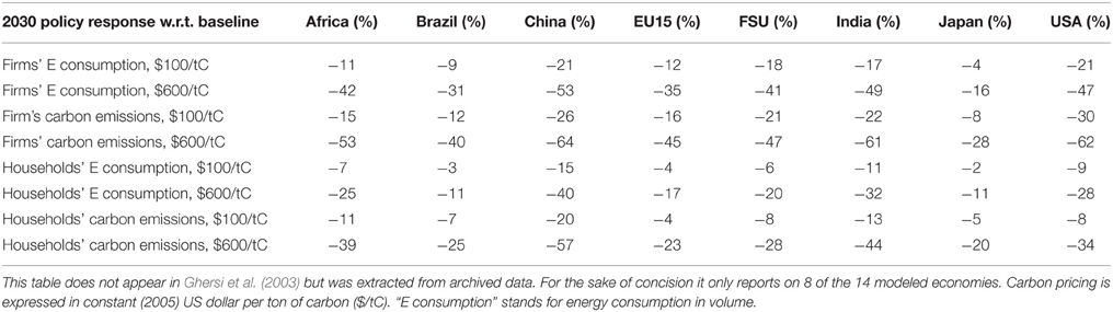
Table 2. Response to carbon pricing of 8 economies in 2030 according to the POLES model.

Accounting for this diversity allows proper elicitation of the winners and losers of the two, somewhat polar policy courses explored—although one important conclusion of the paper is that assessments differ whether considering aggregate GDP (a commonly used measure of efficiency) or induced carbon pricing (an arguable measure of implicit distributive impacts). The analysis is further enriched by considering free vs. auctioned allocation of emission allowances, together with the existence or not of an international market for permits, which also impact on the comparison of allowance rules.

The main methodological shortcoming of this first hybrid modeling endeavor is that it does not build on hybrid energy-economy tables: we disaggregate the 1995 GTAP tables that form our core input-output data using the standard assumption of normalized prices; as a consequence we distort the distribution of energy consumptions across agents (cf. Section Data Harmonization Requirements Building Hybrid Energy/economy Accounting Tables above). Ultimately, by calibrating reduced forms on distorted data we misuse the information extracted from POLES runs.

The Continued Fable of the Elephant and Rabbit

In 2006 we publish the central methodological piece of our hybrid modeling endeavor (Ghersi and Hourcade, 2006), which details the method surveyed in Section Calibration of Reduced Forms of Bottom-up Behaviors above and illustrates its significance at a global scale in 2030, with the purpose of contesting that the “elephant and rabbit stew” of Hogan and Manne (1977) should necessarily taste so much like the former, massively larger animal. The linked bottom-up model is again the POLES model and the runs on which we calibrate global reduced forms are those runs which already fed our 2003 publication (cf. Section Reconciling the Equity and Efficiency of International Burden-sharing Climate above).

Ironically, the response surfaces extracted from POLES for the composite sector and households' energy consumptions turn out quite compatible with the standard CES functions to which we compare our envelope approach: the late 1990s version of POLES that delivered these responses is still only bottom-up from an energy supply point of view—indeed we demonstrate the inability of CES functions to accommodate its responses concerning the energy and capital intensities of energy production—while energy demands largely remain governed by econometric specifications well replicated by CES functions. For this reason we also calibrate our reduced forms on an ALTER dataset, which is in fact a modified POLES dataset with increased curvatures and explicit absolute floors to the 3 energy intensities we work on. We refer to these floors as “technical asymptotes.”

For the sake of argument, our year-2030 policy runs explore a wide range of carbon taxes in the simplified setting of perfect markets, including that of labor, and under the assumption of lump-sum recycling of the carbon tax proceeds to households. Besides the original IMACLIM-S model resorting to reduced forms according to Section Calibration of Reduced Forms of Bottom-up Behaviors, we implement a standard static CES model “CES Kfix” considering an exogenous stock of capital (following, e.g., Böhringer, 1998) and a “CES Kvar” variant of this model, which (1) sorts out the various components of value-added net of labor costs and values its depreciation part as the composite good; (2) treats depreciation as an index of capital demand, which must be balanced by investment.

Even in the controlled environment of perfect markets and lump-sum recycling, IMACLIM-S modeling results for the 2030 global economy turn out to diverge from those of the CES Kfix or CES Kvar approaches. What is more, the sign and magnitude of divergences varies whether GDP, households' non-energy consumption or the marginal cost of decarbonization are considered, as well as whether the POLES or ALTER calibration data is used. For limited ranges of decarbonization and for one or the other indicator the Kvar or Kfix approaches can deliver estimates reasonably close to the IMACLIM-S computation; however they never simultaneously match on the 3 retained indicators and often diverge by up to 100%, thereby justifying the effort invested in a proper modeling of induced production frontiers.

An Outlook on the Macroeconomic Impacts of Electric Vehicles Penetration in EU28

In the framework of a recent EV-STEP research program we developed the coupling of IMACLIM-S with the TIMES PanEU model of the University of Stuttgart, to explore the macroeconomic consequences of accelerated penetration of electric vehicles in the EU28 economy. We worked on a geographically aggregated EU28 but disaggregated 12 productions: 5 energy vectors, 2 types of vehicles (conventional vehicles and electric cars), 1 electric equipment good, which encompasses the batteries of electric vehicles; 3 transportation services (air, water, and land) and 1 composite good, which aggregates all remaining economic products and services⁴².

We implemented the iteration-to-convergence coupling method of Section Coupling Through Iterative Convergence of Linking Variables Trajectories above with a high level of detail, eventually forcing in IMACLIM-S 39 different trajectories either directly taken from TIMES or inferred from its results. These trajectories cover international energy prices, energy exports, primary energy outputs, energy intensities and households' energy demands, but also the capital intensity of the electricity production, the transport services intensity of the composite good (based on ton-kilometer data from TIMES), the transport services demand of households (based on passenger-kilometer data from TIMES), the “electric vehicle intensity” of GDP (uniformly applied to all production sectors) or the actual vehicle demand of households, and indeed the assumed trajectory of battery costs, which we apply to the electric equipment intensity of the electric car production.

Despite the care taken to ground IMACLIM-S on hybrid economy/energy accounts following Section Building from IEA Energy Balances and Energy Price Data above, the data imports from TIMES into IMACLIM-S systematically take the form of trends developing from 2007 on, to be applied to IMACLIM-S variables, rather than of absolute values. The main reason for this is that TIMES PanEU is calibrated on 2005 data, and thus does not match the statistics of further years, including the 2007 data on which IMACLIM-S is calibrated. Another reason is that some non-energy variables, as vehicle sales or transport activities, are not described in IMACLIM-S with the same level of detail as they are in TIMES. A last reason is that we lacked time, in the limited course of a first collaborative, to scan the extensive content of TIMES PanEU for more focused information that we might have used in IMACLIM-S in a more direct way.

We implemented IMACLIM-S for 4 scenarios developed by TIMES PanEU (Table 3) as well as for an optimistic variant on electric cars (EC) exports for the 3 scenarios where EC sales pick up: REF, EU- and EU. Because iterating to convergence was out of the scope of this first research collaborative with the University of Stuttgart, we had to content ourselves with calibrating IMACLIM-S growth under the REF- scenario (the closest to a baseline) on the GDP trajectory common to all 4 TIMES PanEU scenarios. To do so we adjusted the labor productivity gains and export trends of IMACLIM-S to have it replicate the TIMES PanEU GDP trajectory under constraint of its REF- forecast of energy systems. The subsequent runs of the REF, EU- EU scenarios and their EC-exporting variants were developed with unchanged growth drivers, but also without convergence. As a consequence the results reported below are only preliminary results, which at least overestimate those scenario impacts that are imported as variations of total volumes⁴³.

TABLE 3

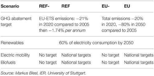
Table 3. Overview of 4 scenarios explored by TIMES PanEU.

Under our pessimistic assumptions on the competitiveness of the EU electric car (EC) industry⁴⁴, EC penetration negatively impacts growth for both the mitigation contexts we explore (Table 3 above), but only slightly so (Figure 5, left panel): in the REF context, the GDP loss of the REF scenario over its REF- counterpart is highest in 2030 at 0.17%. In the EU context, the GDP loss is highest in 2025 at 0.25%. Detailed modeling results and sensitivity analysis reveal that the main cause of the GDP loss is thus not the forced higher penetration of durably more expensive electric cars, which is strongest in 2050 in the REF context and in 2045 in the EU context, but rather the impact of increased electric mobility on energy and especially electricity prices, which culminates at dates corresponding with peaking GDP losses: the REF scenario induces a maximum 1.4% increase in electricity prices over the REF- scenario in 2030, whereas the EU scenario induces a maximum 3.6% increase in electricity prices over the EU- scenario in 2025.

FIGURE 5

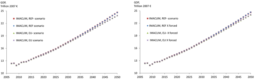
Figure 5. EU28 growth trajectories under 4 scenarios and 3 forced exports variants. Computed from year-to-year real variations according to a chained Fischer GDP price index.

EC production in optimistic (hereafter v2) scenarios strongly exceed EC productions in their original (hereafter v1) counterparts⁴⁵. The impact on GDP is of course not as straightforward as the multiplication of extra exported units by export price, because EC production competes for inputs with other sectors. One exception is however the model's imperfect labor market, where EC production finds unemployed resources to put to use. This is one important mechanism through which the v2 assumptions favorably impact growth. Another major mechanism is international trade: v2 assumptions guarantee substantial exports (and lesser imports) regardless of terms-of-trade competition⁴⁶; they thus lift some pressure off the trade balance, which allows EU prices appreciating vis-à-vis international prices and thus diminishing the brunt of imports.

As a consequence, in 2050 the GDP of REF v2 ends up 0.2% above that of REF v1; that of EU- v2, 0.6% above EU-v1; and that of EU v2, 0.8% above EU v1 (cf. right vs. left panel of Figure 5). In the case of REF, the v2 variant indeed induces a GDP trajectory significantly above that of the REF- v1 scenario: under our modeling assumptions and in the context of moderate climate policy objectives, an optimistic development of international demand for EU-produced electric cars does more than compensate the increased electricity investment needs prompted by EC penetration. Besides, in the ambitious framework of a “factor 5” mitigation objective, favorable assumptions on the competitiveness of the emerging EU electric car industry turn the moderate costs of increased EC penetration (maximum loss of 0.25% GDP in 2025 between the EU- v1 and EU v1 scenarios) into moderate benefits (maximum benefit of 0.10% GDP in 2050 from the EU- v2 to the EU v2 scenario).

The main strength of this coupling exercise is how the aggregate EU28 macroeconomic framework of IMACLIM-S can lean on the 28-country detail of energy systems of TIMES PanEU. Particularly, the impact of electric vehicle penetration on electric systems is assessed at a level of detail that warrants proper modeling of actual regional supply constraints. It is hard to imagine that any CGE framework extended to BU electricity supply could perform in comparable manner.

However, one important limitation of the coupling exercise is the paradigm gap between the simulation, recursive framework of IMACLIM-S, where economic agents take “myopic” decisions only concerned with the state of the economy at the current year, and the optimization framework of TIMES PanEU, where some benevolent planner perfectly anticipates the model's multiple trajectories up to its temporal horizon and accordingly adapts all investment decisions to minimize the total discounted cost of the energy system⁴⁷. Mixing the two approaches could be acceptable if TIMES PanEU modeled energy supply alone, for which centralized energy planning is still the norm in many countries—with the obvious limitation that no central planner has infallible knowledge of the future of energy prices, energy demands and energy technology developments. But TIMES PanEU extends to all end-uses and thus models the investment decision of every single household regarding, e.g., its vehicle or heating equipment. Our coupling experiment must therefore not be interpreted beyond what it really is: a somewhat patchwork outlook on possible energy/economy futures combining macroeconomic simulation and energy system optimization. It was nonetheless a rich experiment of extending to as many variables as possible the connection of IMACLIM-S to a BU model, which can serve in future coupling with simulation models as POLES.

Sovereign Risk and Energy: The RISKERGY Program

Our latest hybrid modeling endeavor is part of the RISKERGY research program, which aims at developing a method of sovereign risk rating that pays due attention to energy issues. The bottom-up model to which we couple IMACLIM-S is again the POLES simulation model but in its most recent version. The requirements of the program prompt us to favor the dynamic framework of the iteration-to-convergence method of Section Coupling Through Iterative Convergence of Linking Variables Trajectories. The purpose is indeed to test the resilience of economies to and the impact on public debt accumulation of short-term shocks along the growth trajectory to 2020.

One key constraint on our research is that our modeling must apply indistinctly to the entire set of countries individualized in POLES, i.e., to close to 50 economies with widely different economic and energy characteristics. As a consequence we have so far worked on aggregate 2-sector economies, although we might disaggregate the energy good in the 4–5 usual vectors in future work. We have also been careful to systematically resort to international datasets covering a large number of countries (at the World Bank, the IMF, the IEA, etc.) to feed our modeling framework with parameters as recent statistical trajectories of GDP growth, labor supply, labor productivity, unemployment but also the trade balance and prevailing exchange rates.

We calibrate our multiple IMACLIM-S country models at the 2007 base year on hybrid matrixes resulting from the combination of the extensive GTAP database (cf. footnote 38 above) with POLES data, following the synthetic method presented Section Building from BU Model Variables at Base Year above. In this instance, shortcutting the alternate extensive method of Section Building from IEA Energy Balances and Energy Price Data appears particularly relevant, considering the daunting task of extending this method to several dozen countries, many of which suffering from poor statistical apparatus. As we already stressed this comes at the cost of some approximations, particularly in the split between households' and firms' transport fuel consumptions.

Working on short term sovereign debt accumulation requires unusual alignment on available statistics. The Solow growth engine we mobilize, despite the path-dependency imposed by importing energy system constraints from POLES, but also statistics on investment, capital utilization and exchange rates, would “miss” the massive 2008 global economic crisis if it were to run on long-term trends of labor productivity improvements only. For this reason, from our 2007 base year up to 2013 and for all country models we perform an original targeting of 3 core macroeconomic statistics (GDP, unemployment, and the trade balance) by adjusting a set of shocks on capital and labor productivities, the negotiation power of workers (which impacts endogenous equilibrium unemployment via a wage curve) and international trade. Beyond 2013 we phase out the crisis perturbations at a constant rate up to 2020 rather than abruptly canceling them, which would induce a somewhat artificial break of macroeconomic trends.

We have so far produced only preliminary runs of the coupled model on the 10 richest world economies, for a baseline as well as for a scenario of oil supply shock, which envisages a 15-million barrel drop of the daily exports of Persian Gulf countries in 2016. POLES and IMACLIM-S converge at 1% (IMACLIM-S computes a GDP impact of updated POLES data below 1%) after 3 iterations only, but for the quite wrong reason that we still have to extend the data imports from POLES to IMACLIM-S to elements other than international energy prices, energy consumptions and intensities—first and foremost to the capital intensity of energy supply, which our applied work on the EU identifies as one major channel of impact of energy systems on growth (cf. Section An Outlook on the Macroeconomic Impacts of Electric Vehicles Penetration in EU28 above).

Although at this early stage of development our coupled model behaves in interpretable manner for all 10 contrasted economies, in the baseline scenario as well as in the oil shock scenario. Compare, e.g., how France and Russia fare facing the 2016 oil shock supply (Figure 6), which translates into a fivefold increase of the international oil price and a consecutive three- to fourfold increase of international gas prices (depending on regional markets). France, highly dependent on oil imports, marks a 3.2% recession in 2016, from which it only partially recovers from 2017 on when the restriction on oil supply lifts and prices fall back to baseline levels or indeed slightly below. Conversely Russia, as major oil and gas exporter, strongly benefits from the price hike induced by the shock. The impact is masked in 2016 because of degraded conditions in Russia's trading partners, but is manifest in later years, as the country reaps the profits of its 2016 investment boost⁴⁸.

FIGURE 6

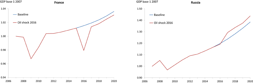
Figure 6. GDP trajectories of France and Russia under baseline and oil shock scenario, IMACLIM-S and POLES coupled modeling.

Similar to Section Reconciling the Equity and Efficiency of International Burden-sharing Climate Agreements but all the more striking in a geographically disaggregated setting, the main force of the coupling is how it allows extending the analysis to a large number of countries with properly characterized energy systems. Such coverage at such level of precision is unquestionably out of reach of standard (non-hybrid) approaches, whatever their macroeconomic paradigm, be it only for the simple reason that the available literature is quite far from providing the country-specific parameterization that should sustain it.

Conclusion and Further Research Agenda

It is our hope that this survey demonstrates significant advances in our ability to propose hybrid modeling solutions to the energy and climate modeling challenge. Over the last 15 years we have outlined and have started implementing two operational methods of coupling extensive bottom-up modeling to our IMACLIM-S macroeconomic framework. We have also addressed data harmonization issues to guarantee the relevance of model dialogue, which has incidentally led us to model agent-specific prices, a significant improvement over other TD modeling endeavors. Our numerical applications are few but growing, and should shortly benefit from the contributions of other authors on the Brazilian and South African economies.

Some unsettled issues naturally require further research. Regarding data harmonization and the production of hybrid base year accounts, we still have to settle on a more satisfactory treatment of energy auto-consumptions. The issue depends on whether we are hybridizing in link with disaggregated energy balances or with the coupled BU model. The high level of disaggregation of IEA balances allows proper identification of the genuine energy inputs (for consumption or transformation) of all energy sectors—notwithstanding whether these end up aggregated or not. The decision is then easier made to strip down auto-consumptions to genuine marketed inputs, or to identify, by comparing energy with national accounting data, putative commodity trade, which can then be given specific modeling. Hybridizing base year data by importing energy expenses and volumes from the coupled BU model offers less choice because of a lasting simplification of BU models: these rarely distinguish between crude oil and petroleum products, which forbids pinpointing the crude oil expenses of the refining industry—one major auto-consumption of the aggregate energy sector of hybrid accounts built on BU data. However, the refining data are readily available from even aggregated IEA balance sheets and could be exploited in future work.

Our coupling methods also call for further developments. The calibration of reduced forms is conceptually stabilized, but only in the case of an aggregate and “closed” (global) economy. Questions remain as to how to extend the method to a multisectoral setting. Similar to the two-sector setting but with increased degrees of freedom, a prerequisite is to settle on some conceptual form for the instantaneous trade-offs between inputs or consumptions. The implication of such choice on modeling results remains to be assessed. Another particularly open field of investigation regards households' consumptions: in the wake of the research on aggregate macroeconomic models boiling down to some aggregate production function, E3 modelers have devoted much attention to the producer's side of the energy conservation problem and very little to the consumer's side of it, as testifies the poor treatment of households energy trade-offs in current models⁴⁹.

The iteration-to-convergence method is also quite advanced, although it has developed in a more pragmatic way. However, our provisory treatment of trade-offs other than those involving energy is too standard and we must at the very least move to a modeling of capital vintages with putty-clay characteristics, lest the benefits of importing explicit energy systems inertias be lost in a too lax treatment of substitution possibilities for non-energy factors. The feedback from IMACLIM-S to the coupled BU model can also surely be expanded to more than GDP or other activity indicators. As we hint at the end of Section Coupling Through Iterative Convergence of Linking Variables Trajectories, IMACLIM-S computes endogenous relative prices for all factors of production, which, if transmitted to the capital and operation & maintenance costs identified by BU models for all technologies, could turn out to alter the “merit order” of technologies.

Conflict of Interest Statement

The author declares that the research was conducted in the absence of any commercial or financial relationships that could be construed as a potential conflict of interest.

Footnotes

1 ^Notwithstanding, bottom-up models have been criticized for their too-naive representation of supply or demand technologies investment decision (Sutherland, 1991)—the source of a perceived “efficiency gap” between the available techniques and those really implemented (Jaffe and Stavins, 1994), quite unsatisfactorily explained by extremely high private discount rates. The CIMS model provides some answers to this issue (Jaccard, 2009), which is however beyond our scope here.

2 ^Berndt and Wood are among the first to estimate a Capital, Labor, Energy, Materials, or KLEM production function of the aggregate United States economy (research leading to Berndt and Wood, 1975). As early as 1974, Jorgenson publishes a multisectoral KLEM model of the United States, which he applies to a prospective outlook up to the year 2000 (Hudson and Jorgenson, 1974).

3 ^Löschel (2002) reviews technical change in economic models of climate or energy policy of the 1990s.

4 ^Equipment stocks are understood in the broadest sense here. Consider notably the impact of urban forms, which evolve over centuries, on the share of individual vs. collective housing (with obvious consequences on heating requirements) or on the substitutability of public to private transport.

5 ^Kennedy explicitly builds on Hicks: “A change in the relative prices of the factors of production is itself a spur to invention and to inventions of a particular kind—directed at economizing the use of a factor which has become relatively expensive” (Hicks, 1932, p. 124). The work of Kennedy spurred much literature up to Magat (1979), which includes a thorough review.

6 ^Figure 1 is taken from Ghersi and Hourcade (2006), where it is further commented upon.

7 ^Cohen and Harcourt (2003) provide a thorough review from a viewpoint similar to our own.

8 ^See e.g., McFarland et al. (2004), Sue Wing (2006), Laitner and Hanson (2006), Schumacher and Sands (2007), Böhringer and Rutherford (2008), Fujimori et al. (2014), Cai et al. (2015).

9 ^This section draws on Ghersi and Hourcade (2006).

10 ^The POLES model is jointly developed by CNRS, IPTS, and ENERDATA, cf. http://edden.upmf-grenoble.fr/spip.php?article1471.

11 ^Figure 2 proposes scenario range alternatives to the carbon tax issue. These remain to be explored in future work.

12 ^In the implicitly “constant” (deflated) currency of POLES.

13 ^The method applied in Ghersi et al. (2003) differs in its more complex treatment of capital. We succinctly explain how in Section Reconciling the Equity and Efficiency of International Burden-sharing Climate Agreements below.

14 ^In Ghersi and Hourcade (2006) we detail our method of projection of use and resource tables under constraint of energy system information.

15 ^The non-energy variable costs of energy production reported by POLES provide an estimate of the sum of material and labor costs. Because the labor content of energy production is low, its response to relative prices shifts can be neglected at a macroeconomic level. Changes in the non-energy intermediate consumption of new techniques may be more significant, but are not reported by the state-of-the-art of BU models—if they were, they could easily find their way into our methodology.

16 ^In Ghersi and Hourcade (2006) we resort to the least-square adjustment of an arctangent specification, purposely selected to allow reproducing asymptotes to substitution possibilities.

17 ^Interest payments are a percentage of equipment expenditures that is easily computed by setting an average lifespan of capital and a constant rate of growth of equipment expenditures together with a constant real interest rate over this lifespan—the two rates being assumed equal on a stabilized growth path.

18 ^E.g., in models as G-Cubed, MS-MRT, SGM, EPPA. Cf. respectively McKibbin and Wilcoxen (1995), Bernstein et al. (1999), Fisher-Vanden et al. (1993), Babiker et al. (2001).

19 ^Note that the assumptions of constant expenditures, constant composite consumption and constant composite price are incompatible with variations of the energy expenditures. Given necessarily constant non-energy prices, we prefer to consider a constant income (more compatible with the fixed GDP assumption of POLES) rather than a constant consumption of the composite good.

20 ^Because energy models increasingly account for the impacts of learning-by-doing and R&D efforts on the costs of energy technologies, the envelope of energy production functions is assumed to embody such effects and is therefore not subject to productivity adjustments.

21 ^We calibrate the specification to allow a doubling of cumulated investment triggering a 20% cost decrease, based on 1978–2000 time-series for France and OECD. Sensitivity analyses demonstrate that variations of the elasticity of total factor productivity to real investment do not qualitatively affect the model.

22 ^In a TD framework the consumer and GDP price indexes come to mind as deflators of respectively the consumer's and producer's carbon taxes. Because the two indexes generally do not match, one uniform tax of the BU framework translates into two distinct taxes in the TD framework—which does not simplify policy analysis or the interpretation of modeling results. Besides, both deflators are endogenous to the TD framework. Ultimately, the carbon pricing trajectory sustaining any modeling output of IMACLIM-S with reduced forms is not easily pinpointed.

23 ^The approach is similar to that of Dai et al. (2015) but with data exchange extended to prices; or to that of Fortes et al. (2014) or Labriet et al. (2015), although energy prices, rather than exogenously taken from the bottom-up source, remain largely endogenous variables of IMACLIM-S (cf. below). The idea of coupling economic and energy models via iteration of linking variables exchanges up to convergence dates back at least to Hoffman and Jorgenson (1976). It was picked up throughout the years to present times (cf., e.g., Messner and Schrattenholzer, 2000; Schäfer and Jacoby, 2006; Martinsen, 2011) where it appears to flourish (cf. the above 3 recent papers but also Igos et al., 2015).

24 ^Contrary to the endogenous primary resources markets of the global multiregional version of IMACLIM, IMACLIM-R (Sassi et al., 2010).

25 ^In disaggregated version the composite M is an aggregate of non-energy goods, whose trade-off we must again settle resorting to some behavioral assumption. In the applied work reported Section An Outlook on the Macroeconomic Impacts of Electric Vehicles Penetration in EU28 we fall back on the Leontief assumption of fixed intensities.

26 ^Van der Werf (2008) and Okagawa and Ban (2008) econometrically establish the superiority of the chosen structure over other possible choices (i.e., substituting K to E then the KE aggregate to L). They also are precious sources of estimation of the elasticities of substitution of CES functions at each tier of the structure.

27 ^In disaggregated version, this E intensity is a vector of energy intensities reflecting some energy mix.

28 ^In both the applied works of Section An Outlook on the Macroeconomic Impacts of Electric Vehicles Penetration in EU28 and Sovereign Risk and Energy: The RISKERGY Program we do so by assuming an inverse evolution of imports and exports, which we apply to gross imports and exports volumes of the calibration year as reported by IEA balances.

29 ^This iteration is embedded in the larger iteration of linking variables exchanges between models, i.e., it is performed for each run of IMACLIM-S under updated constraints from the linked BU model. In the case of the applied work of Section An Outlook on the Macroeconomic Impacts of Electric Vehicles Penetration in EU28 convergence of cost trajectories at a 10⁻³ precision requires in the order of 5 iterations of capital productivity changes.

30 ^The year at which the model is calibrated to match national accounts statistics.

31 ^Surprisingly enough, the French national statistics institute (INSEE) indicates that “product transfers” impact but a few sectors, mainly related to agriculture (INSEE, 2012). The 4 energy sectors of the 88-sector INSEE IO table are indeed barely concerned by product transfers corrections, and in a positive way only (which means that some firms mainly involved in non-energy activities have a minor share of their activity on energy markets). This implies that energy firms do not sell anything but energy products strictly speaking, an arguably questionable statistics.

32 ^This section draws on yet unpublished research co-authored with Emmanuel Combet, Julien Lefévre, and Gaëlle Le Treut at CIRED.

33 ^In their most disaggregated format IEA energy balances detail 71 resources and uses for 60 energy products.

34 ^For example, the 2010 IO table of France by INSEE reports a 45 billion Euro auto-consumption of the gas and electricity production and distribution sector. This is incompatible with the ca. 8 million ton-of-oil equivalent (toe) consumptions of said industries reported by the IEA energy balance–which cannot be valued at more than €1000 per toe on average.

35 ^In our applied work on the European Union (cf. Section An Outlook on the Macroeconomic Impacts of Electric Vehicles Penetration in EU28), sectoral disaggregation has prompted us to move commodity trade from the energy sectors to the composite sector (which includes trading activities). Conversely, in the sectorally aggregated but geographically extensive framework of our RISKERGY work (cf. Section Sovereign Risk and Energy: the RISKERGY Program) we have decided to rather adjust the auto-consumption of our aggregate energy sectors prorata the adjustment of other energy uses by the hybridizing process (cf. Section Building from BU Model Variables at Base Year below).

36 ^CIRED makes frequent use of the ENERDATA database at http://www.enerdata.net.

37 ^National accounts treat the energy consumptions of public administrations as these of an aggregate public service sector, whose uses focus on the final consumption of public administrations. For this reason, the direct final energy consumptions of public administrations are nil. Understandably, gross fixed capital formation does not consume (immobilize) any energy flow either, at least notwithstanding stock variations (cf. above).

38 ^In the 8.1 version we used, GTAP details harmonized 57-sector input-output tables for 134 countries or regions covering the globe, cf. https://www.gtap.agecon.purdue.edu/databases/v8/default.asp (accessed July 2015).

39 ^In the applied work of Section Sovereign Risk and Energy: The RISKERGY Program we crudely attribute to households all fuel consumptions of light duty vehicles. A non-negligible part of such consumptions are paid for by firms, though. Conversely, some fuel consumptions attached to light trucks but also to boats and even airplanes (although statistically negligible) are paid for by households.

40 ^All numerical applications reported here, boiling down to the resolution of either one single set (at time horizon T) or a succession of sets (from time 0 to time horizon T) of simultaneous non-linear equations, are successfully conducted in Microsoft Excel with the help of the Excel solver. Depending on sectoral disaggregation, the number of solver variables varies between 12 and 67 (with many more variables functions of these).

41 ^Löschel (2002) stresses how most CGE modelers set key elasticity of substitution parameters judgmentally rather than based on genuine economic analysis. The later rare econometric efforts of Van der Werf (2008) and Okagawa and Ban (2008) offer limited regional coverage that falls short of concerning the 14 global regions of our hybrid modeling.

42 ^In Ghersi (2014) we thoroughly describe the construction of a hybrid energy-economy EU28 matrix and lay out the coupling method, although not in its ultimate refinements. In Ghersi (2015) we publish scenario results together with appendixes describing complementary data mining and treatment, ultimate amendments to the model and the complete detail of the data imports from the TIMES PanEU model.

43 ^I.e., variations of households' energy consumptions and of energy exports. Impacts on firms' consumptions are imported as intensities, which minimizes divergence between the first iteration and the ultimate converged equilibrium. Note that the volume output of primary energies is probably exogenous to TIMES scenarios, which also reduces divergence between the first and the converged iteration.

44 ^One industry that does not export and that, at base year, imports half its domestic sales from abroad, whereas conventional vehicles are only for 8% of them imported goods.

45 ^Optimistic export scenarios consider (1) vehicle exports climbing from 10 to 200% of vehicle sales to households between 2008 and 2020, then remaining at 200% of household sales up to 2050; (2) an aggregate vehicle import share at base year identical to that of conventional vehicles, i.e., of 8% rather than 50%.

46 ^To give an order of magnitude: 10 million vehicles at 25 thousand Euros amounts to €250 billion exports; the REF v2, EU- v2, and EU v2 scenarios respectively reach 7, 25, and 27 million units exports. In the REF- v1 scenario, EU exports start from ca. €1,700 billion in 2007 and climb to €5,600 billion in 2050.

47 ^Schäfer and Jacoby (2006), Martinsen (2011) (although not iterating to convergence) or Labriet et al. (2015) have similarly coupled optimisation models of the MARKAL family with recursive TD models.

48 ^Results are for the polar case of fixed exchange rates, which implies that the boost in trade balance causes households' consumption to shrink relative to investment and public consumptions (with these fixed shares of GDP and consumption its remainder). In further research we will envisage some flexible representation of terms-of-trade.

49 ^E.g., the DART (Klepper et al., 2003), EPPA (Paltsev et al., 2005), PACE (Böhringer, 2002), or the PHOENIX model (Sue Wing et al., 2011) still resort to nested CES functions to represent consumer demand. The nesting commonly isolates one aggregate energy bundle from all other consumptions, thus leveling off both the substitution possibilities among energy goods on one side and those between the energy bundle and the bundle of all non-energy goods on the other side. Cai et al. (2015) circumvent some of these limitations by resorting to CRESH functions rather than CES functions in their GTEM-C model. Schäfer and Jacoby (2005) or Karplus et al. (2013), both implementing the EPPA model of the MIT, are rare examples of an elaborate treatment of household demand (concerning private car).

References

Bauer, N., Edenhofer, O., and Kypreos, S. (2008). Linking energy system and macroeconomic growth models. Comput. Managem. Sci. 5, 95–117. doi: 10.1007/s10287-007-0042-3

CrossRef Full Text | Google Scholar

Babiker, M. H., Reilly, J. M., Mayer, M., Eckaus, R. S., Sue Wing, I., and Hyman, R. C. (2001). The MIT Emissions Prediction and Policy Analysis (EPPA) Model: Emissions, Sensitivities and Comparison of Results. Joint Program on the Science and Policy of Global Change report #71, Cambridge, MA: Massachusetts Institute of Technology. Available online at: http://web.mit.edu/globalchange/www/MITJPSPGC_Rpt71.pdf (accessed July 2015)

Berndt, E. R., and Wood, D. O. (1975). Technology, prices, and the derived demand for energy. Rev. Econ. Stat. 57, 259–268. doi: 10.2307/1923910

CrossRef Full Text | Google Scholar

Bernstein, P. M., Montgomery, W. D., and Rutherford, T. F. (1999). Global impacts of the Kyoto agreement: results from the MS-MRT model. Res. Energy Econ. 21, 375–413. doi: 10.1016/S0928-7655(99)00009-3

CrossRef Full Text | Google Scholar

Böhringer, C. (1998). The synthesis of bottom-up and top-down in energy policy modeling. Energy Econ. 20, 233–248. doi: 10.1016/S0140-9883(97)00015-7

CrossRef Full Text | Google Scholar

Böhringer, C. (2002). Climate politics from Kyoto to Bonn: from little to nothing? Energy J. 23, 51–71. doi: 10.5547/ISSN0195-6574-EJ-Vol23-No2-2

CrossRef Full Text | Google Scholar

Böhringer, C., and Rutherford, T. F. (2008). Combining bottom-up and top-down. Energy Econ. 30, 574–596. doi: 10.1016/j.eneco.2007.03.004

PubMed Abstract | CrossRef Full Text | Google Scholar

Cai, Y., Newth, D., Finnigan, J., and Gunasekera, D. (2015). A hybrid energy-economy model for global integrated assessment of climate change, carbon mitigation and energy transformation. Appl. Energy 148, 381–395. doi: 10.1016/j.apenergy.2015.03.106

CrossRef Full Text | Google Scholar

Cohen, A. J., and Harcourt, G. C. (2003). Whatever happened to the cambridge capital theory controversies? J. Econ. Perspect. 17, 199–214. doi: 10.1257/089533003321165010

CrossRef Full Text | Google Scholar

Dai, H., Mischke, P., Xie, X., Xie, Y., and Masui, T. (2015). Closing the gap? Top-down versus bottom-up projections of China's regional energy use and CO₂ emissions. Appl. Energy. doi: 10.1016/j.apenergy.2015.06.069. Available online at: http://www.sciencedirect.com/science/article/pii/S0306261915008272. [Epub ahead of print].

CrossRef Full Text

Fisher-Vanden, K., Edmonds, J. A., Pitcher, H. M., Barns, D., Baron, R., Kim, S., et al. (1993). The Second Generation Model of Energy Use, the Economy, and Greenhouse Gas Emissions. Washington, DC: Pacific Northwest Laboratory. 17. Available online at: http://sedac.ciesin.org/mva/FV1993/FV1993.html (accessed July 2015).

Fortes, P., Pereira, R., Pereira, A., and Seixas, J. (2014). Integrated technological-economic modeling platform for energy and climate policy analysis. Energy 73, 716–730. doi: 10.1016/j.energy.2014.06.075

CrossRef Full Text | Google Scholar

Fujimori, S., Masui, T., and Matsuoka, Y. (2014). Development of a global computable general equilibrium model coupled with detailed energy end-use technology. Appl. Energy 128, 296–306. doi: 10.1016/j.apenergy.2014.04.074

CrossRef Full Text | Google Scholar

Ghersi, F. (2014). Macroeconomic Modeling of Electrified Mobility Systems in 2030 European Union. CIRED Working Paper 55-2014. Paris: CIRED. 32. Available online at: http://www.centre-cired.fr/IMG/pdf/CIREDWP-201455.pdf

Ghersi, F. (2015). Macroeconomic Modeling of Electrified Mobility Systems in 2030 European Union. Scenario Results. CIRED Working Paper 58-2015. Paris: CIRED. 32. Available online at: http://www.centre-cired.fr/IMG/pdf/ciredwp-201458.pdf

Ghersi, F., and Hourcade, J.-C. (2006). Macroeconomic consistency issues in E3 modeling: the continued fable of the elephant and the rabbit. Energy J. S2, 39–62. doi: 10.5547/issn0195-6574-ej-volsi2006-nosi2-3

CrossRef Full Text | Google Scholar

Ghersi, F., Hourcade, J.-C., and Criqui, P. (2003). Viable responses to the equity-responsibility dilemma: a consequentialist view. Clim. Policy 3S1, S115–S133. doi: 10.1016/j.clipol.2003.10.011

CrossRef Full Text | Google Scholar

Grubb, M., Edmonds, J., ten Brink, P., and Morrison, M. (1993). The costs of limiting fossil-fuel CO₂ emissions: a survey and analysis. Ann. Rev. Energy Environ. 18, 397–478. doi: 10.1146/annurev.eg.18.110193.002145

CrossRef Full Text | Google Scholar

Hicks, J. R. (1932). The Theory of Wages. London: MacMillan.

Hoffman, K. C., and Jorgenson, D. (1976). Economic and technological models for evaluation of energy policy. Bell J. Econ. Managem. Sci. 8, 444–466. doi: 10.2307/3003296

CrossRef Full Text | Google Scholar

Hogan, W. W., and Manne, A. S. (1977). “Energy-economy interactions: the fable of the elephant and the rabbit?” in Modeling Energy-Economy Interactions: Five Approaches, ed C. J. Hitch (Washington, DC: Resources for the Future), 247–277.

Hourcade, J.-C., Jaccard, M. K., Bataille, C., and Ghersi, F. (2006). Hybrid modeling: new answers to old challenges. Energy J. S2, 1–12. doi: 10.5547/ISSN0195-6574-EJ-VolSI2006-NoSI2-1

CrossRef Full Text | Google Scholar

Hourcade, J.-C., and Shukla, P. (2001). “Global, regional and national costs and ancillary benefits of mitigation,” in Climate Change 2001: Mitigation, eds B. Metz, O. Davidson, R. Swart, and J. Pan (Cambridge: Cambridge University Press), 499–559.

Hudson, E. A., and Jorgenson, D. W. (1974). U. S. energy policy and economic growth, 1975-2000. Bell J. Econ. Managem. Sci. 5, 461–514. doi: 10.2307/3003118

CrossRef Full Text | Google Scholar

Igos, E., Rugani, B., Rege, S., Benetto, E., Drouet, L., and Zachary, D. S. (2015). Combination of equilibrium models and hybrid life cycle-input–output analysis to predict the environmental impacts of energy policy scenarios. Appl. Energy 145, 234–245. doi: 10.1016/j.apenergy.2015.02.007

CrossRef Full Text | Google Scholar

INSEE. (2012). Méthodologie des Comptes Trimestriels. INSEE Méthodes 126. Paris: Institut National de la Statistique et des Études Économiques. 143.

Jaccard, M. K. (2009). “Combining top down and bottom up in energy economy models,” in International Handbook on the Economics of Energy, eds J. Evans and L. C. Hunt (Cheltenham: Edward Elgar), 311–331.

Jaffe, A. B., and Stavins, R. N. (1994). The energy-efficiency gap. What does it mean? Energy Pol. 22, 804–810. doi: 10.1016/0301-4215(94)90138-4

CrossRef Full Text | Google Scholar

Karplus, V. J., Paltsev, S., Babiker, M., and Reilly, J. M. (2013). Applying engineering and fleet detail to represent passenger vehicle transport in a computable general equilibrium model. Econ. Model. 30, 295–305. doi: 10.1016/j.econmod.2012.08.019

CrossRef Full Text | Google Scholar

Kennedy, C. (1964). Induced bias in innovation and the theory of distribution. Econ. J. 74, 541–547. doi: 10.2307/2228295

CrossRef Full Text | Google Scholar

Klepper, G., Peterson, S., and Springer, K. (2003). DART97: A Description of the Multi-regional, Multi-sectoral Trade Model for the Analysis of Climate Policies. Kiel Working Papers 1149, Kiel Institut für Weltwirtschaft, Kiel. 40. Available online at: http://www.ifw-members.ifw-kiel.de/publications/dart97-a-description-of-the-multi-regional-multi-sectoral-trade-model-for-the-analysis-of-climate-policies [accessed December 2014].

Labriet, M., Drouet, L., Vielle, M., Loulou, R., Kanudia, A., and Haurie, A. (2015). Assessment of the Effectiveness of Global Climate Policies Using Coupled Bottom-up and Top-down Models. Nota di Lavoro 23.2015. Milan: Fondazione ENI Enrico Mattei. 22.

Google Scholar

Laitner, J. A. S., and Hanson, D. A. (2006). Modeling detailed energy-efficiency technologies and technology policies within a CGE framework. Energy J. S2, 151–169. doi: 10.5547/issn0195-6574-ej-volsi2006-nosi2-8

CrossRef Full Text | Google Scholar

Löschel, A. (2002). Technological change in economic models of environmental policy: a survey. Ecol. Econ. 43, 105–126. doi: 10.1016/S0921-8009(02)00209-4

CrossRef Full Text | Google Scholar

Magat, W. A. (1979). Technological advance with depletion of innovation possibilities - implications for the dynamics of factor shares. Econ. J. 89, 614–623. doi: 10.2307/2231871

CrossRef Full Text | Google Scholar

Manne, A. S. (1977). ETA-MACRO: A Model of Energy-Economy Interactions. NASA STI/Recon Technical Report, 78, 26612.

Martinsen, T. (2011). Introducing technology learning for energy technologies in a national CGE model through soft links to global and national energy models. Energy Pol. 39, 3327–3336. doi: 10.1016/j.enpol.2011.03.025

CrossRef Full Text | Google Scholar

McFarland, J. R., Reilly, J. M., and Herzog, H. J. (2004). Representing energy technologies in top-down economic models using bottom-up information. Energy Econ. 26, 685–707. doi: 10.1016/j.eneco.2004.04.026

CrossRef Full Text | Google Scholar

McKibbin, W., and Wilcoxen, J. (1995). The theoretical and empirical structure of the G-Cubed model. Brookings discussion paper in International Economics, 118.

Google Scholar

Messner, S., and Schrattenholzer, L. (2000). MESSAGE–MACRO: linking an energy supply model with a macroeconomic module and solving it iteratively. Energy 25, 267–282. doi: 10.1016/S0360-5442(99)00063-8

CrossRef Full Text | Google Scholar

Okagawa, A., and Ban, K. (2008). Estimation of substitution elasticities for CGE models. Discussion Papers in Economics and Business 08-16, Graduate School of Economics and Osaka School of International Public Policy (OSIPP), Osaka: Osaka University. Available online at: http://www2.econ.osaka-u.ac.jp/library/global/dp/0816.pdf (accessed July 2015)

Paltsev, S., Reilly, J. M., Jacoby, H. D., Eckaus, R. S., McFarland, J., Sarofim, M., et al. (2005). The MIT Emissions Prediction and Policy Analysis (EPPA) model: Version 4. MIT Joint Program on the Science and Policy of Global Change, Report 125, Cambridge, USA. 78. Available online at: http://globalchange.mit.edu/files/document/MITJPSPGC_Rpt125.pdf [accessed December 2014].

Ruttan, V. (2002). “Sources of technical change: Induced innovation, evolutionary theory, and path dependence,” in Technological Change and the Environment, eds A. Grübler, N. Nakicenovic, and W. D. Nordhaus (Washington, DC: Resources for the Future), 9–39.

Sassi, O., Crassous, R., Hourcade, J.-C., Gitz, V., Waisman, H., and Guivarch, C. (2010). IMACLIM-R: a modeling framework to simulate sustainable development pathways. Inter. J. Glob. Environ. Iss. 10, 5–24. doi: 10.1504/IJGENVI.2010.030566

CrossRef Full Text

Schäfer, A., and Jacoby, H. D. (2005). Technology detail in a multisector CGE model: transport under climate policy. Energy Econ. 27, 1–24. doi: 10.1016/j.eneco.2004.10.005

CrossRef Full Text | Google Scholar

Schäfer, A., and Jacoby, H. D. (2006). Experiments with a hybrid CGE-MARKAL model. Energy J. S2, 171–177. doi: 10.5547/issn0195-6574-ej-volsi2006-nosi2-9

CrossRef Full Text

Schumacher, K., and Sands, R. D. (2007). Where are the industrial technologies in energy–economy models? An innovative CGE approach for steel production in Germany. Energy Econ. 29, 799–825. doi: 10.1016/j.eneco.2006.12.007

CrossRef Full Text | Google Scholar

Solow, R. M. (1957). Technical change and the aggregate production function. Rev. Econ. Stat. 39, 312–320. doi: 10.2307/1926047

CrossRef Full Text | Google Scholar

Solow, R. M. (1959). “Investment and technical progress,” in Mathematical Methods in the Social Sciences, eds K. J. Arrow, S. Karlin, and P. Suppes (Stanford, CA: Stanford University Press), 89–104.

Sue Wing, I. (2006). The synthesis of bottom-up and top-down approaches to climate policy modeling: electric power technologies and the cost of limiting US CO2 emissions. Energy Pol. 34, 3847–3869. doi: 10.1016/j.enpol.2005.08.027

CrossRef Full Text | Google Scholar

Sue Wing, I., Daenzer, K., Fisher-Vanden, K., and Calvin, K. (2011). Phoenix Model Documentation. Maryland: Joint Global Change Research Institute, University of Maryland. 84. Available online at: Http://www.globalchange.umd.edu/data/models/phx_documentation_august_2011.pdf [accessed December 2014].

Sutherland, R. (1991). Market barriers to energy efficiency investments. Energy J. 12, 15–34. doi: 10.5547/ISSN0195-6574-EJ-Vol12-No3-3

CrossRef Full Text | Google Scholar

Van der Werf, E. (2008). Production functions for climate policy modeling: an empirical analysis. Energy Econ. 30, 2964–2979. doi: 10.1016/j.eneco.2008.05.008

CrossRef Full Text | Google Scholar