Modeling Exposure of Mammalian Predators to Anticoagulant Rodenticides

Introduction

Anticoagulant rodenticides (AR) are a widespread and effective method of rodent control (WHO, 1995; Erickson and Urban, 2004; Laakso et al., 2010). AR are slow-acting toxins that block vitamin K regulating blood's ability to clot. The poisoned animals typically die as a result of internal bleeding 8–10 days after ingesting a lethal dose of poison. The development of resistance to the poisons (e.g., warfarin and coumatetralyl) in rodents led to the development of the more toxic “second-generation” AR (Pelz, 2001; Lodal, 2010; Vein et al., 2011). These second-generation compounds are also metabolized and excreted more slowly than their predecessors. They tend to accumulate in liver and can have very long internal half-lives (e.g., 307 days for brodifacoum (Vandenbroucke et al., 2008). These second-generation ARs therefore pose an increased risk of secondary poisoning of small mammal predators (Alterio, 1996; Berny et al., 1997; Newton et al., 1999; Erickson and Urban, 2004; Dowding et al., 2010; Laakso et al., 2010). In fact the risk of secondary poisoning is well known and was described for first generation compounds in the 1960s (Evans and Ward, 1967). Subsequently, studies in the laboratory and the field have documented lethal effects of secondary exposure to AR in predators (Alterio et al., 1997; Berny et al., 1997; Murphy et al., 1998; Giraudoux et al., 2006; Dowding et al., 2010; Walker et al., 2010).

Small-mammal predators (mustelids and birds) assayed for exposure to AR in Denmark have an incidence of exposure of 84–100% depending upon species (Elmeros et al., 2011; Christensen et al., 2012). Not only was the percentage of animals exposed high in the Danish predators, but in most species there were individuals (up to 70%) with rodenticide concentrations in the liver above (200 ng/g live-weight); a potentially lethal concentration for mustelids and birds of prey (Grolleau et al., 1989; Newton et al., 1999). Some predators also had concentrations that are associated with lethal toxic effects in the fox, 800 ng/g live-weight (Berny et al., 1997).

Rodenticide concentration levels in weasels and stoats suggests Danish animals have a higher occurrence of positives and higher concentrations in Denmark than found in other European countries (Shore et al., 2003; Elmeros et al., 2011), although this to a certain may be accounted for by differential sensitivity of the analytical techniques. High rates and concentrations of AR in predators have similarly been found in France and New Zealand in association with intensive rodent control campaigns (Alterio, 1996; Alterio et al., 1997; Berny et al., 1997; Murphy et al., 1998; Eason et al., 1999).

The cause of the very high rates of AR in non-target predators in Denmark is not known. The predators assayed previously were collected during a period when the use of AR to combat rodents in forests, tree crops, and game feeding stations was allowed (Elmeros et al., 2011; Christensen et al., 2012). In 2010, the Danish EPA changed the regulations and prevented use of rodenticides in woodland and tree-crops by the end of 2011. The aim was in part to reduce the prevalence of rodenticide in non-target organisms, and was based on the assumption that use in these habitats conferred the highest risk of exposure (i.e., contact between the non-target animal and the rodenticide). However, a recent assay found that there was no decrease in prevalence of AR in either stone marten or polecat. On the contrary, the AR burden in stone marten increased from 1999–2004 to 2012–2013, while it remained constant in polecats (Elmeros et al., 2015).

In this study we consider two possible hypotheses to explain the almost universal exposure of predators in Denmark. The first was that rodent vectored rodenticide might spread far enough to become available to the majority of predators; the second being that the pattern of household and urban use might be enough in itself to explain the intensive secondary exposure of predators. We also consider whether the regulation changes in 2010 should have been enough to reduce exposure of non-targets significantly by removing rodenticides from woodlands and other uses away from buildings.

The primary focus of this study was the development of model representing the coincidence of predators and rodenticide in time and space. However, to support the model a study of how far mice might vector rodenticide using mark-release-recapture was also undertaken. The modeling tool included dynamic modeling of the fate of rodenticide, baiting frequency, timing and placement, and estimation of predator territory density and locations at 1-m² resolution on three 10 × 10-km landscapes. Finally, the real-world impact of new Danish regulations was evaluated using a new survey of rodenticide concentrations found in Danish mammalian small-mammal predators (Elmeros et al., 2015), post the new rodenticide restrictions imposed by the Danish EPA. This data was also used to compare to model predictions.

Materials and Methods

Capture-Mark-Recapture

To elucidate on the potential rodent vectored rodenticide dispersal away from baiting sites to become available in a larger area to the majority of small mammal predators, we determined dispersal distances of small rodents during the autumn, when rodenticide use is most intensive in Denmark.

Dispersal distances of anticoagulant rodenticide poisoned mice and voles from a bait box were assessed by capture-mark-recapture over an 8 week period in two study areas during the autumn (mid-September–mid-November) 2012. Rodents were caught in Ugglan multiple-capture live-traps. The traps were baited with ample food (apples and unhusked seeds) and supplied hay as bedding material and checked once a day. Traps were positioned on the ground sheltered by vegetation, i.e., protected from extreme weather. A solid lid on the traps provided cover from exposure to precipitation and wind. The two study areas (75 × 200 m) comprised patches of herbs, shrubs, and trees. The areas were delimited by local landscape features and contained 147 and 149 traps, respectively. Within each study area the traps were evenly distributed 15 × 15 m apart around each baiting station. Individual rodents weighing >15 g were marked subcutaneously with a small PIT-tag (Passive Integrated Transponder, Oregon RFID). Individuals below 15 g were not tagged on ethical grounds. Hence, only dispersal distances for rodents >15 g were recorded. Mice and voles were trapped and marked during two 5-day trapping sessions with 2 week intervals and a final trapping session in the 7th and 8th week.

Dispersal distances between captures (all inter-trap distances) of small mammals were compared between species and study areas by generalized linear mixed modeling.

ALMaSS

The model was developed within ALMaSS (Topping et al., 2003), an agent-based simulation system utilizing a highly configurable and detailed landscape model component (Topping et al., 2016). ALMaSS is an open source C++ project, and all code is available through the GitLab¹. In addition, documented code using ODdox documentation for the rodenticide model is available via an internet link². The rodenticide model was created partly utilizing the existing landscape sub-model which was extended to handle baiting location coding and rodenticide baiting timing and frequencies (see below). The complete model was developed by creating two further sub-models to enable rodenticide handling within the landscape (represented by the Rodenticide and the RodenticidePredator C++ classes in the program). These classes implemented all other behavior necessary for the rodenticide model (see ODdox²). The overall modeling strategy was somewhat similar to (e.g., Nogeire et al., 2015) in that we attempted to create distributions of predators based on habitat structure and then overlay exposure. The main differences were that we had no predator population dynamics, the scale which is much smaller in our study and more detailed, and that we used a more detailed simulation of baiting patterns, and subsequent AR vectoring and environmental decay.

Landscape Maps

To evaluate the variability associated with landscape structure, all scenarios were run on three different 10 × 10 km landscapes with differing compositions representing real rural Danish landscapes (see Supplementary Material). These landscapes represent a small field, locally heterogeneous regionally homogenous landscape (Herning), a typical estate landscape with large fields and large wooded areas (Præstø), and an intermediate landscape (Bjerringbro).

Mouse-Vectored Rodenticide Simulation

Rates of mouse dispersal when vectoring rodenticide were assumed to be the same as dispersal rates measured from the capture-mark-recapture study (see Results section). Rates of dispersal were somewhat varied for the different species of rodent. However, maximum distance moved only varied little between species. The dispersal rates were considered as a diffusion process from a point source. Since variation in maximum distance moved between the three sets of curves was small only the yellow-necked mouse data was used for fitting and subsequent scenarios. To fit this diffusion process to the 2-dimensional representation required by the model, the curve of frequency of distance moved was used to calibrate the model procedure.

The equation used to model diffusion evaluates the amount of rodenticide present in a single cell at a time. It is assumed that diffusion processes in all directions operate equally and that at each time step of one day a fixed proportion (p) of the rodenticide present (a_t) is distributed to all surrounding cells. The rate and distance of travel is also determined by two other parameters, d is the cell width in meters, and D is the assumed to be the rate of decay resulting in a half-life of the rodenticide after bait placement. This is primarily meant to represent an internal half-life once ingested by mice, but will also operate on the baiting location to remove rodenticide assumed to be as a result of other routes (e.g., rats, slugs). At each time step the amount of rodenticide leaving a cell (a_o) is given by Equation (1). This amount is divided equally between all cells of size d bordering the current cell.

$\begin{array}{ll}{a}_o=(a_t(1-D))p& (1)\end{array}$

The amount of rodenticide entering a cell is given by the sum of the amounts leaving all surrounding cells. The change in rodenticide amount per cell is given by Equation (2).

$\begin{array}{ll}{a}_{t+1}={\displaystyle \underset{k=0}{\sum ^n}}{a}_{ok}+a_t-a_o& (2)\end{array}$

where k is the number of surrounding cells.

Parameters p and d were varied and used to calibrate the diffusion model to fit as closely as possible to the mouse dispersal data. Evaluation of fit was by using a least squares estimation resulting in three sets of parameters. Fits were reasonably good, although not perfect (Figure 1). In all cases the fit was made ignoring the 0–10 m category, since the step-wise nature of the model introduced excessive noise when diffusion to so few cells was included, especially since cell sizes of 5 × 5 m were found to provide the best fits.

FIGURE 1

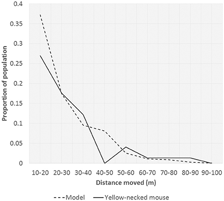
Figure 1. Yellow-necked mouse dispersal distances and fitted diffusion model.

Landscape Coding and Bait Locations

To determine the bait locations from a landscape map, the map features were classified into types of potential bait locations and other features. The ALMaSS map is polygon-based, and as such each element is represented by a polygon and classified into 55 element types. Potential bait locations were determined to be buildings, woodlands, and Christmas tree plantations. These elements were identified and a central point lying inside each polygon found by calculating the center of the minimum sized rectangle which could surround the polygon and then searching outward in a spiral pattern from this point until a location was found inside the polygon in question. The spiraling was only needed in the cases where polygons had other areas within them (e.g., doughnut shaped).

Buildings required a further step to classify them as urban or country buildings since these have different baiting profiles. All buildings were initially designated as urban. Then the minimum distance to the nearest 6 other buildings was calculated for each building. The building was reclassified as country if this minimum distance exceeded 100-m. The values of 100-m and 6 buildings were determined by visual inspection of the resulting classification on the Bjerringbro map before fixing these values for all simulations.

Each baiting location was designated a type based on the polygon type, thus four categories of baiting location were created (woodland, Christmas trees, country buildings, and urban building). Each baiting location also had type-dependent annual probability of bait placement (i.e., the annual chance that bait is used at all at this location), and a seasonal distribution of likely bait placement dates (i.e., a probability based distribution of date of placement if used). During a simulation the annual bait placement probability was used at the beginning of each year to determine whether bait was placed at that point in that year—if so the date was selected from a type-specific list of potential baiting dates. The list of dates comprised of a set of 365 daily probabilities summing to 1.0. Seasonal baiting could therefore be simulated by weighting or zeroing probabilities of bait placement for individual dates or periods. Once bait was placed it was assumed to be present at the point source for a type-specific period; these periods being determined by estimates of treatment times from professional pest-control practitioners (see Scenario Development below). Once a bait location had been active for the designated period it was assumed to be used up or removed and thus no further bait would be added resulting in a slow degradation of bait the rate dependent upon the half-life parameter D (see Equation 1).

Predator Modeling

Predator modeling consisted of two separate processes: The first was to define predator territories where exposure to rodenticide could be evaluated. The second stage was collection of exposure information during the scenario runs.

Defining predator territories: Predator home-ranges (H-R) were assumed to be square. Determination of a territory was calculated separately for each predator type by the model based on three criteria:

1) That the sum of the scores of the areas contained within the H-R exceeded a minimum level, representing the habitat resources needed by each species. The H-R score was built up of individual scores for each 1-m² or each habitat within the territory. The habitat score was based on the landscape element type indexing a species specific set of landscape element type scores (e.g., a stone marten will score a building higher than a pine marten). The value of the scores were determined by expert judgment and fitting of the territories to the Bjerringbro landscape. These scores were then also used for the Præstø and Herning landscapes to generate predator territory maps.

2) That the home-range size achieving the score was between a maximum and minimum size (measured as width), and based on literature estimates for each species (Table 1);

3) That the territory did not overlap with another predator territory;

TABLE 1

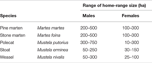
Table 1. Typical home-range (H-R) sizes of mustelids in Denmark based on European studies (see Supplementary Table 2).

Predator territories were created for each map once, and stored for future use in all scenarios. Hence, it is possible to directly compare exposure between landscapes within a species. The method of territory creation was to start randomly within one maximum territory distance, but not less than half the territory width, from the NW corner of the map and evaluate whether a minimum sized territory centered on that location fulfilled the above criteria. If so the territory was placed and the map area claimed (could not be used for new territories). If it was not possible to create a territory the territory size was incremented the procedure repeated until either maximum size was reached or it was possible to place the territory. At this point the next map location to the east was selected and the procedure repeated. If there were no more locations to the east then the first location on the row one south was selected and the procedure repeated. Once all locations had been evaluated then the procedure was halted and the map finalized. Example territory locations are shown in Figure 2. Each time this procedure was applied slightly different maps were generated, but initial testing indicated that the variation due to this factor was negligible.

FIGURE 2

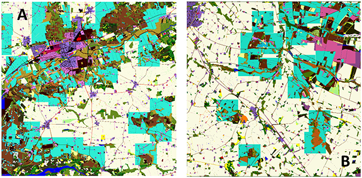
Figure 2. Example predator territory locations (overlay in blue) in two 10 × 10 km landscape maps, Bjerringbro (A) and Herning (B) for M. nivalis. In this case territories are clustered around semi-natural landscape elements and avoid town areas and open country. The territories are represented as squares of a minimum size required to achieve the minimum territory score based on the area of underlying habitats.

Evaluating predatory territory exposure: This was achieved by creating an index of exposure based on the mean daily total amount of mouse-vectored rodenticide present in the territory. Each day during the simulation every 1 × 1-m grid cell was evaluated for rodenticide exposure and the total summed for the whole territory. At the end of the simulation the total was divided by the number of days counted and saved as output. This statistic is not real exposure, but an index of the available rodenticide in a territory, hereafter referred to as an “exposure index.”

Scenario Development

There was no available systematic survey on the frequency and duration of treatment nor the between year variation in the pattern of rodent control in Denmark. The values for the annual frequency, time of year and the duration of baiting in different landscape elements included in the model were determined from interviews and assessments with professional pest control, rat consultants, and former users of rodenticides in forestry and Christmas tree production. Information on length of baiting period was obtained in the form of x% for 1 month, y% for 2 months, and z% for 6 months. The mean length of baiting was therefore calculated as:

$\begin{array}{ll}days=(30x+60y+180z)/100& (3)\end{array}$

Default frequency, length and timing of baiting is given by Table 2. All scenarios were run on all three landscapes, with a default half-life of 14-days unless otherwise specified below. In all cases 100 replicates of 1 year of each scenario were run, enough to ensure mean exposures were stable (within 1%) on addition of further replicates. In all cases, the likelihood of baiting a location (e.g., an urban building) in the model depends firstly on the annual by area probability (5%) for an urban building. If bating will occur then there is a probability applied determining the time of year it is baited, and then the bait is simulated in the model for the baiting length from Equation (3).

TABLE 2

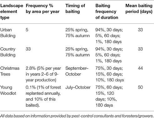
Table 2. The default frequency, timings of start of baiting and baiting duration used for the all scenarios unless otherwise specified.

Experiments

Experiment 1—Evaluation of Present and Past Exposure

The main set of simulations was carried out for five species (Martes martes, Martes foina, Mustela putorius, Mustela ermine, Mustela nivalis), on all three landscapes and consisted of two scenarios. Scenario 1 (baseline) assumed the standard situation prior to 2012, where pesticides were used in wooded areas and Christmas trees. Scenario 2 (present day), assumed the same distribution and frequency of baiting locations for buildings, but zero rodenticide usage in Christmas trees and woodlots. In all scenarios the half-life of rodenticide exposure was set to be 14 days and frequency and timing of baiting set to the standard conditions described by the consultants.

Experiment 2—Sensitivity to Environmental Half-Life

The half-life parameter is not as simple as a normal environmental half-life since it covers the availability of the rodenticide to the predators. This includes the concentration in mice before they die, and any storage of contaminated food which may be eaten later, as well as whether dead mice may be consumed. Half-life in the mice (e.g., of bromadiolone) is 28 days (Vandenbroucke et al., 2008), with other typical 2nd generation rodenticides varying between 16 and 307 days. For all main scenarios we chose a half-life of 14 days (conservative for estimating exposure), but carried out a sensitivity analysis for two species (M. foina and M. nivalis) varying half-life to be 7, 14, 28, and 56 days.

Experiment 3—Baiting Frequency

One of the largest uncertainties present in determining the exposure is the frequency of baiting. Therefore, a third experiment was run to determine the sensitivity of the results to the frequency of baiting. Two additional baiting frequencies were considered for M. foina and M. nivalis, at 50 and 25% the frequency suggested by the consultants.

Analysis

Analysis was performed on the potential rodenticide exposure index as calculated by each predator territory. Means were calculated for each scenario from all predator territories present in the landscape (between 10 and 40 depending upon species and landscape). All statistics were calculated by pooling all 100 replicates for each species used. The number of territories that were unexposed (exposure index = 0.0) was also recorded and the proportion of these calculated. These indicate zero exposure within 1 year, but do not necessarily mean that the territory was not exposed between years.

Results

Mark Release Recapture

A total of 220 bank voles (Myodes glareolus), 63 field voles (Microtus agrestis) and 66 yellow-necked mice (Apodemus flavicollis) were marked, and 561, 77, and 74 recaptures were recorded. Mean dispersal distances between recaptures of yellow-necked mice, bank voles and field voles were 20.2 ± 18.0 m, 11.2 ± 13.2 m, and 9.0 ± 10.7 m (Table 3). Yellow-necked mice dispersed further than the other species (Table 4).

TABLE 3

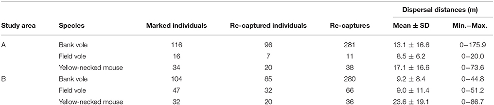
Table 3. Summary of dispersal distances of marked mice and voles over 8 weeks during autumn 2012.

TABLE 4

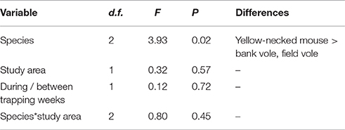
Table 4. Relationship between dispersal distances of marked mice and voles, species, study areas and trapping sessions as determined by GLMM.

Experiment 1: Evaluation of Present and Past Exposure

The major result of these simulations is that a very low percentage of predator territories have zero exposure to rodenticides. The cessation of use of rodenticides in woodland and Christmas tree areas is predicted to have an effect on the total exposure index, but only a very minor impact on the proportion of territories unexposed (Table 5). The highest proportion of unexposed territories was 3.14% in Herning for M. nivalis, but across all cessation scenarios there was a mean of 0.29% and median of 0.00%. Figure 3 shows a map of the exposure index in the Bjerringbro landscape in late September, when rodenticide levels are at the peak. There is a concentration in the town area, but very few areas are not exposed across the landscape.

TABLE 5

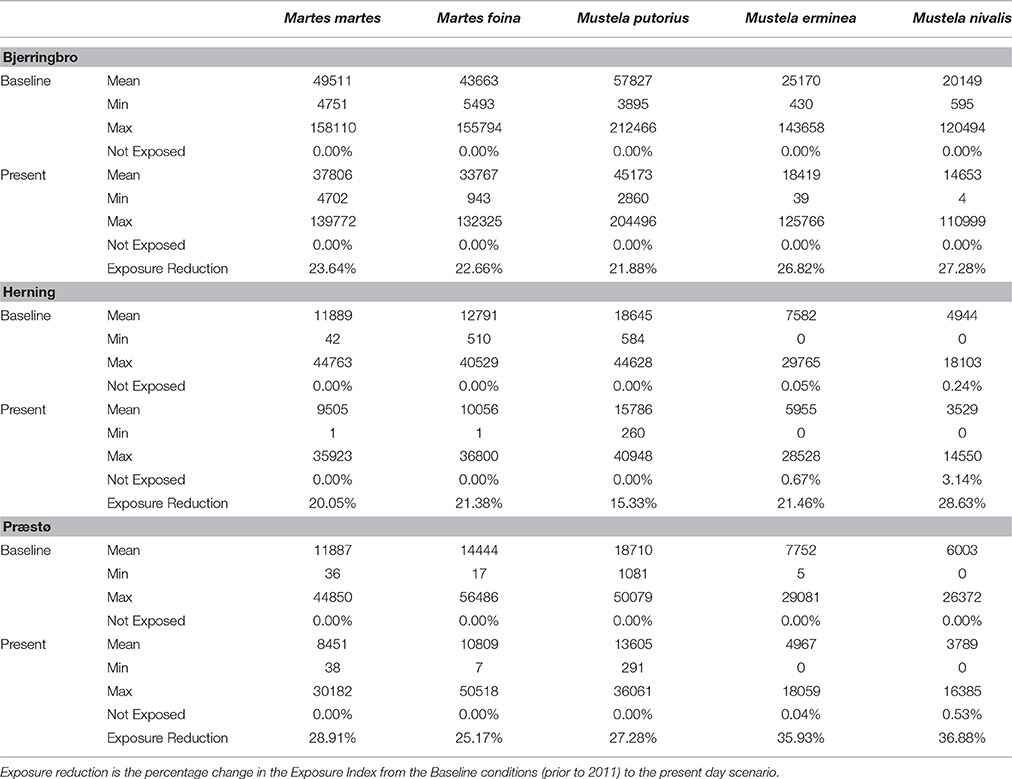
Table 5. Results of Experiment 1 for the each of the three landscapes as exposure indices.

FIGURE 3

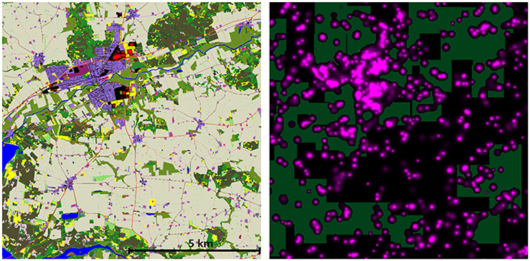
Figure 3. Map of the Bjerringbro landscape (left) and an AR exposure map from September 30th for Scenario 2 (present day). Colored areas indicate modeled AC environmental concentration on this day. Note the distribution of AR does not allow for placement of the M. nivalis territories shown as light rectangles without covering one or more AR locations. See also Supplementary Material for a time-series of this data as a video showing the spatio-temporal dynamics of AR availability in the landscape.

Mean exposure index values differed markedly between species as a function of location and size of territory, with highest exposure in polecat (M. putoris) and lowest in weasel (M. nivalis). This is as expected simply due to differences in H-R sizes, but there was also a sizeable variation between landscapes, with exposure values for Bjerringbro being 3–4 times higher than Herning and Præstø. Cessation of woodland and Christmas tree treatment reduced mean exposure index scores by 15–37% with highest reductions in the weasel, and lowest reductions on average in the polecat.

Coefficient of variation increases noticeably on cessation of woodland use of rodenticides. This is in keeping with the higher variability expected, especially in the predators with smaller territories and less association with human habitation (e.g., stoat and weasel), but impacts were seen for all species. This suggests that although still exposed there was a greater variation in exposure following cessation, indicating a positive impact greater than suggested by the reduced percentage of territories with zero exposure.

Experiment 2: Sensitivity to Environmental Half-Life

Increasing or decreasing half-life increased or decreased the exposure index close to proportionally, a second order polynomial having a perfect fit to the data (e.g., Bjerringbro M. foina y = −7.0655x2 + 1192.4x − 720.89, R² = 1). However, even with a 7-day half-life, the proportion of territories unexposed was very low, close to zero for M. foina and between zero, and 5% for M. nivalis, depending upon the landscape (Table 6).

TABLE 6

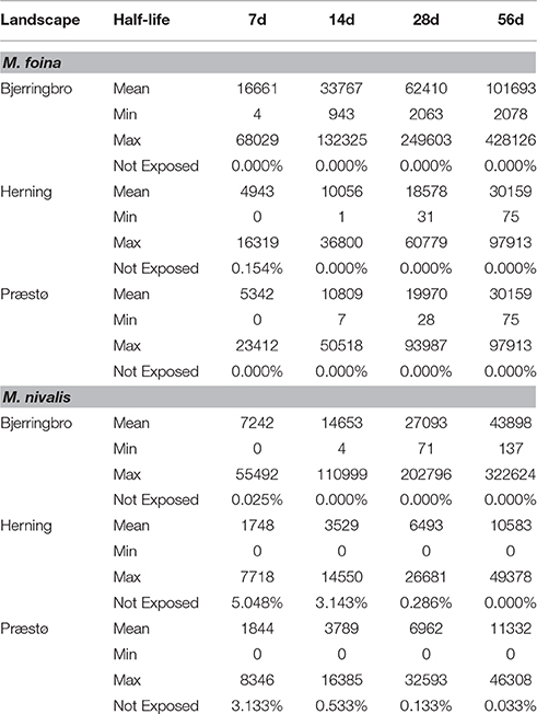
Table 6. The effects of varying the environmental half-life parameter on exposure of M. foina and M. nivalis for three landscapes.

Experiment 3: Baiting Frequency

Altering the assumptions related to the baiting frequency by reducing the frequency by 50 and 75% reduced the mean index of exposure linearly with the reduction in baiting frequency for both M. foina and M. nivalis (Figure 4). The rate of reduction was different in Bjerringbro compared to Herning and Præstø due to the higher predicted exposure in that landscape. Reductions in the number of territories not exposed were also predicted but these were not linear and for M. foina reductions of 75% were needed to achieve increases in unexposed territories of just over 0.5% in Bjerringbro, with maximum reductions of 4% in Herning. Præstø was intermediate between these two; for M. nivalis the reductions were greater, but not proportionally so. Maximum reductions were also in Herning (almost 12%), but reductions in Præstø were only slightly lower. In Bjerringbro, even at 75% reduced baiting frequency more than 99% of weasel territories were exposed (Figure 4).

FIGURE 4

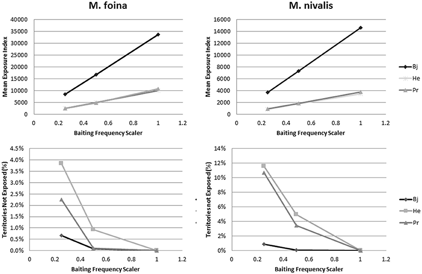
Figure 4. Changes in mean exposure index and the percentage of territories not exposed when reducing the frequency of baiting to 50 and 75%. Bj, Bjerringbro; He, Herning; Pr, Præstø landscapes respectively. Each point is a based on multiple replicates, but with very small standard errors (not graphed).

Discussion

Model Uncertainties

The results of the overall modeling exercise are very clear. There are few if any predators moving around the Danish landscape that do not have the potential to be exposed to rodenticide even if rodenticides are only used for rat control in and around buildings. There are, however, a number of key uncertainties in the model to take into account, the main ones being the frequency of baiting, the patterns of rodenticide vectoring, the pattern of predator territories, and the extent to which potential exposure can be translated to real exposure. We have characterized these with respect to their effect on predicted impact.

Uncertainties that will Tend to Under-Estimate Impact with the Present Scenario:

• We have assumed only two types of baiting are present in the landscapes, urban and rural buildings. The frequency of baiting is therefore simplified to these two types, whereas in reality baiting may be more diverse (e.g., industrial units, sewers). The frequency may also be under or over estimated. Under estimation will not alter results significantly since results suggest that almost 100% of territories are exposed and this situation cannot be made much worse. If the frequency estimates are over-estimated then for weasels there may be an important effect in some landscapes. However, it does not seem likely that the professional pest control experts would make errors of the magnitude needed to create these effects (i.e., 400% too large), and even at this level of error very few territories will be unexposed (0–12% depending on species and landscape).

• There are also uncertainties regarding the distribution of rodenticide poisoned rodents. We assume it is vectored by mouse movement but take no account of changed mouse behavior which would under estimate exposure in the model if poisoned mice were easier to catch (Cox and Smith, 1992), and might affect the proportion of contaminated rodents in the diet. The diffusion model for rodent rodenticide dispersal compares well with recorded dispersal distances of poisoned small mammals during standard rat control operations with bait stations on farms (Geduhn et al., 2014). Dispersal distances of mice and voles are probably underestimated in these studies as individuals that moved away from the trapping grid were not recorded. Yellow-necked mice may disperse >1 km in one night (Stradiotto et al., 2009), i.e., potentially carrying poisoning long distance into the surrounding areas.

• We also assume 100% mouse and vole vectoring as these small rodents are the most dominant in the mustelid diet (Clevenger, 1994; Lode, 1997; Elmeros, 2006), but most poison is placed to control rats, and rural rats have much larger home-ranges and longer dispersal ranges than mice and voles (Taylor, 1978; Taylor and Quy, 1978; Lambert et al., 2008). It is also possible that bait is stored by rodents and is therefore available for a longer time than suggested (Jensen and Nielsen, 1986; McKenzie et al., 2005).

• The method of allocating predator territories has not been tested against real data and is based on expert judgment. However, real data on territories required to test the procedures used here is not available and would be difficult to obtain, thus there is little chance of immediate improvement of this part of the model. However, the modeled home-range sizes for the predators are probably underestimated and the fixed locations of H-R do not represent the variation in size and the high plasticity of mustelids foraging habitats.

• The model calculates exposure for a single year, and many predators are long-lived (e.g., maximum lifespan for free-ranging M. foina is >10 years (Ansorge and Jeschke, 1999), thus the life-time chance of exposure is higher than suggested here for the majority of species.

Uncertainties that will Tend to Over-Estimate Impact:

• The pattern of mouse deaths is not taken into account and may reduce rodenticide spread if it's faster than assumed (i.e., if mice die quickly), resulting in a shorter rodenticide environmental half-life than the 14 days used here. However, Experiment 2 suggested a low sensitivity to this parameter.

• Translation of the potential exposure predicted by the model to actual exposure is very difficult. Factors that come into play here are the efficiency of territory search and mouse capture, and the diet choice. For example the diet of stone martens is wider than mice (Clevenger, 1994), whereas weasel is a more specialized rodent predator (Elmeros, 2006). These difficulties mean that comparisons of exposure can only realistically be made within a species (relative exposure).

• We assume that all mice access the bait with equal probability. However, it has been shown that exposure in small mammal species varies in different UK landscapes, probably relating to habitat use and precise bait-box placement (Brakes and Smith, 2005). The direction of this bias is not certain, although, it probably over-estimates impact since some species and locations may reduce accessibility, whereas increasing it is not possible since the model assumes it is fully accessible.

In addition to these uncertainties, there is a general problem that the data against which we compare the model comes from a changing world where not all factors can be controlled. This can clearly be seen when we compare the results of reducing use of AR usage on stone martens, where AR burdens increased (Elmeros et al., 2015). Since there is no obvious mechanism for a decreased frequency and distribution of use to increase exposure it must be the real-world data that is inconsistent. This could be for many reasons, e.g., changing demography of the predators, changing spatial distribution, or most likely, a non-recorded change in baiting effort between the two measurements from the real world. In the case of stone marten and polecat this seems to have resulted in a an underestimate of effect in the model, but the actual effect cannot be known for sure without knowledge of which factors were changing the real world in which direction.

Implications of Results

Since the majority of the uncertainties are conservative, suggesting even higher levels of potential exposure than modeled, it seems reasonable to conclude that very few predators in the Danish landscape will have no chance of exposure to anti-coagulant rodenticide over the course of a year. This conclusion is strongly supported by the empirical evidence of the AR assays for small mammal predators carried out both pre- and post-regulation changes in Danish rodenticide use (Elmeros et al., 2015).

The actual exposure rates will vary with the landscape and species considered, with sparsely human—populated areas having lower exposure risk. But given that the three landscapes used here were typical of rural Denmark, then it is highly unlikely that large areas of the country are free of rodenticide, even after rodenticide use restrictions in woodlots. Cessation of rodenticide use in woodlots and Christmas trees and elsewhere away from building, e.g., game feeding stations has almost certainly reduced overall exposure rates considerably in wooded habitats, but has done little for exposure incidence. However, the assumption of standard baiting amounts may play a role and if significantly bias may alter this conclusion. There currently is no way of knowing whether the amounts of AR used per baiting application were the same in woodlots etc., as it was around buildings, as statistics on AR usage have not been compiled.

Exposure incidence is important because the method used here calculated a mean annual exposure, and thus it does not relate directly to dose. In this system dose is likely to vary considerably with time (Geduhn et al., 2016), since it is the chance encounter with an individual carrying a heavy rodenticide body burden that will determine maximum dose. Hence, toxico-dynamics are an important aspect to consider, and may mitigate against the decrease in Exposure Index if it is in fact AR use around buildings that typically provides these chance encounters.

Reducing the dispersal distances of mice had no significant impact on exposure estimates, and as such although of academic interest unless we consider very great variations in dispersal (e.g., kilometer scales, which would be the case for rats), then the precise form and slope of the dispersal function does not significantly affect exposure incidence in the model. Therefore, of our original two hypotheses explaining the almost universal exposure of predators in Denmark, it seems clear that the primary explanation is that the pattern of household and urban use might be enough in itself to explain the extent of secondary exposure of predators.

Future Model Development

The most important question to answer is what is the effect of exposure to rodenticides on populations of small mammal predators? To answer this requires three further steps.

Firstly we need to develop good models for the toxicological impacts on individuals as a result of receiving a dose of AR. There is little data on dose-response or even toxicity in non-target predators, and indications of very large variability in AR sensitivity in birds (Eason et al., 2002), and poor dose-response relationships in existing data (Rattner et al., 2014), but mammalian studies (e.g., Grolleau et al., 1989) are rare. Secondly, the estimates of exposure should be refined to relate model exposure to real world exposure. Whilst in our model the pattern of bait use is realistically represented, we do not know how this relates to transfer of ARs to predators. A quantitative estimate could be made by relating model predicted exposure correlated with real world body-burdens in space and time, e.g., using legally trapped pest species and road kills. Finally, these components need to be combined with spatio-temporal models of small mammal predator populations. Toxicity and exposure data could be combined to refine the simulation model, including toxico-dynamics, and toxico-kinetics to predict maximum dose. However, to function it will be necessary to map the spatial and temporal dynamics of both ARs in the environment and the predators. For example, there is seasonal variation in the use of farm buildings by polecats, where ARs are used (Birks, 1998), which may explain the increase in AR burdens in polecats in winter in Denmark (Elmeros et al., 2015). Such a population model should be individual-based (e.g., Nogeire et al., 2015), but should also ideally be able to represent environmental and behavioral details accurately to assess individual toxico-kinetics (e.g., Topping et al., 2016). A further improvement would be the use of multiple landscapes for testing scenarios. Recently the highly detailed landscapes used here have become easier to develop (at least for Denmark) (Topping et al, loc.cit) and thus new strategies could be evaluated against a wide range of real situations to evaluate their general applicability.

Ethics Statement

Trapping and tagging of rodents was done in accordance to a permit to trap and tag mammals and birds issued to Department of Bioscience by the Danish Nature Agency: SN 302-009 SEI.

Author Contributions

Both CT and ME contributed to planning and execution of the work as well as to preparation of the manuscript.

Funding

The study was funded by research grants from the Danish Environmental Protection Agency (MST 667-00100 and MST 667-00112).

Conflict of Interest Statement

The authors declare that the research was conducted in the absence of any commercial or financial relationships that could be construed as a potential conflict of interest.

Acknowledgments

Lene Jung Kjær, Jennifer Lynch, Jens Peder Hounisen, Lars Haugaard and Thomas K. Christensen provided valuable technical and field assistance. Peter Weile, the Nature Agency, and private PCOs are thanked for information on AR application patterns. Thanks also to the two reviewers for their helpful comments.

Supplementary Material

The Supplementary Material for this article can be found online at: https://www.frontiersin.org/article/10.3389/fenvs.2016.00080/full#supplementary-material

Footnotes

1. ^https://gitlab.com/groups/ALMaSS

2. ^https://almassdocs.au.dk/ALMaSSODdox/RodenticideModel/index.html

References

Alterio, N. (1996). Secondary poisoning of stoats (Mustela erminea), feral ferrets (Mustela furo), and feral house cats (Felis catus) by the anticoagulant poison, brodifacoum. N. Z. J. Zool. 23, 331–338. doi: 10.1080/03014223.1996.9518092

CrossRef Full Text | Google Scholar

Alterio, N., Brown, K., and Moller, H. (1997). Secondary poisoning of mustelids in a New Zealand Nothofagus forest. J. Zool. 243, 863–869. doi: 10.1111/j.1469-7998.1997.tb01986.x

CrossRef Full Text | Google Scholar

Ansorge, H., and Jeschke, D. (1999). Altersstruktur und Reproduktion des Steinmarders (Martes foina) in der Oberlausitz. Z. Säutetierkd 64(Suppl. 5).

Berny, P. J., Buronfosse, T., Buronfosse, F., Lamarque, F., and Lorgue, G. (1997). Field evidence of secondary poisoning of foxes (Vulpes vulpes) and buzzards (Buteo buteo) by bromadiolone, a 4-year survey. Chemosphere 35, 1817–1829. doi: 10.1016/S0045-6535(97)00242-7

PubMed Abstract | CrossRef Full Text | Google Scholar

Birks, J. D. S. (1998). Secondary rodenticide poisoning risk arising from winter farmyard use by the European polecat Mustela putorius. Biol. Conserv. 85, 233–240. doi: 10.1016/S0006-3207(97)00175-4

CrossRef Full Text | Google Scholar

Brakes, C. R., and Smith, R. H. (2005). Exposure of non-target small mammals to rodenticides: short-term effects, recovery and implications for secondary poisoning. J. Appl. Ecol. 42, 118–128. doi: 10.1111/j.1365-2664.2005.00997.x

CrossRef Full Text | Google Scholar

Christensen, T. K., Lassen, P., and Elmeros, M. (2012). High exposure rates of anticoagulant rodenticides in predatory bird species in intensively Managed Landscapes in Denmark. Arch. Environ. Contam. Toxicol. 63, 437–444. doi: 10.1007/s00244-012-9771-6

PubMed Abstract | CrossRef Full Text | Google Scholar

Clevenger, A. (1994). “Feeding ecology of Eurasian pine martens and stone martens in Europe,” in Martens, Sables and Fishers. Biology and Conservation, eds S. W. Buskirk, A. S. Harestad, M. G. Raphael, and R. A. Powell (New York, NY: Cornell University Press), 326–340.

Cox, P., and Smith, R. (1992). “Rodenticide ecotoxicology: pre-lethal effects of anticoagulants on rat behavior,” in Proceedings of the Fifteenth Vertebrate Pest Conference (Davis, CA: University of California).

Dowding, C. V., Shore, R. F., Worgan, A., Baker, P. J., and Harris, S. (2010). Accumulation of anticoagulant rodenticides in a non-target insectivore, the European hedgehog (Erinaceus europaeus). Environ. Pollut. 158, 161–166. doi: 10.1016/j.envpol.2009.07.017

PubMed Abstract | CrossRef Full Text | Google Scholar

Eason, C. T., Murphy, E. C., Wright, G. R., and Spurr, E. B. (2002). Assessment of risks of brodifacoum to non-target birds and mammals in New Zealand. Ecotoxicology 11, 35–48. doi: 10.1023/A:1013793029831

PubMed Abstract | CrossRef Full Text | Google Scholar

Eason, C. T., Milne, L., Potts, M., Morriss, G., Wright, G. R. G., and Sutherland, O. R. W. (1999). Secondary and tertiary poisoning risks associated with brodifacoum. N. Z. J. Ecol. 23, 219–224.

Google Scholar

Elmeros, M. (2006). Food habits of stoats Mustela erminea and weasels Mustela nivalis in Denmark. Acta Theriol. 51, 179–186. doi: 10.1007/BF03192669

CrossRef Full Text | Google Scholar

Elmeros, M., Topping, C. J., Christensen, T. K., Lassen, P., and Bossi, R. (2015). Spredning af anti-koagulante rodenticider med mus og eksponeringsrisiko for rovdyr. Bekæmpelsesmiddelforskning 159, 67.

Elmeros, M., Christensen, T. K., and Lassen, P. (2011). Concentrations of anticoagulant rodenticides in stoats Mustela erminea and weasels Mustela nivalis from Denmark. Sci. Total Environ. 409, 2373–2378. doi: 10.1016/j.scitotenv.2011.03.006

PubMed Abstract | CrossRef Full Text | Google Scholar

Erickson, W., and Urban, D. (2004). Potential Risks of Nine Rodenticides to Birds and Non-target Mammals: A Comparative Approach, Washington, DC: U.S. Environmental Protection Agency report. EPA Office of Pesticide Programs.

Evans, J., and Ward, J. L. (1967). Secondary poisoning associated with anticoagulant-treated nutria. J. Am. Vet. Med. Assoc. 151, 856–861.

Google Scholar

Geduhn, A., Esther, A., Schenke, D., Gabriel, D., and Jacob, J. (2016). Prey composition modulates exposure risk to anticoagulant rodenticides in a sentinel predator, the barn owl. Sci. Total Environ. 544, 150–157. doi: 10.1016/j.scitotenv.2015.11.117

PubMed Abstract | CrossRef Full Text | Google Scholar

Geduhn, A., Esther, A., Schenke, D., Mattes, H., and Jacob, J. (2014). Spatial and temporal exposure patterns in non-target small mammals during brodifacoum rat control. Sci. Total Environ. 496, 328–338. doi: 10.1016/j.scitotenv.2014.07.049

PubMed Abstract | CrossRef Full Text | Google Scholar

Giraudoux, P., Tremollières, C., Barbier, B., Defaut, R., Rieffel, D., Berny, N., et al. (2006). Persistence of bromadiolone anticoagulant rodenticide in Arvicola terrestris populations after field control. Environ. Res. 102, 291–298. doi: 10.1016/j.envres.2006.02.008

PubMed Abstract | CrossRef Full Text | Google Scholar

Grolleau, G., Lorgue, G., and Nahas, K. (1989). Toxicité secondaire, en laboratoire, d'un rodenticide anticoagulant (bromadiolone) pour des prédateurs de rongeurs champêtres: buse variable (Buteo buteo) et hermine (Mustela erminea). EPPO Bull. 19, 633–648. doi: 10.1111/j.1365-2338.1989.tb01153.x

CrossRef Full Text

Jensen, T. S., and Nielsen, O. F. (1986). Rodents as seed dispersers in a heath—oak wood succession. Oecologia 70, 214–221. doi: 10.1007/BF00379242

CrossRef Full Text | Google Scholar

Laakso, S., Suomalainen, K., and Koivisto, S. (2010). Literature Review on Residues of Anticoagulant Rodenticides in Non-Target Animals Temanord. Copenhagen, Nordic Council of Ministers. 541.

Google Scholar

Lambert, M. S., Quy, R. J., Smith, R. H., and Cowan, D. P. (2008). The effect of habitat management on home-range size and survival of rural Norway rat populations. J. Appl. Ecol. 45, 1753–1761. doi: 10.1111/j.1365-2664.2008.01543.x

CrossRef Full Text | Google Scholar

Lodal, J. (2010). Resistens hos Brune Rotter: Monitering af Resistens hos den Brune Rotte i Danmark 2001–2008. Miljøprojekt 1312, Danish Environmental Protection Agency / Miljøstyrelsen.

Lode, T. (1997). Trophic status and feeding habits of the European Polecat Mustela putorius L. (1758). Mamm. Rev. 27, 177–184. doi: 10.1111/j.1365-2907.1997.tb00447.x

CrossRef Full Text | Google Scholar

McKenzie, T. L., Bird, L. R., and Roberts, W. A. (2005). The effects of cache modification on food caching and retrieval behavior by rats. Learn. Motiv. 36, 260–278. doi: 10.1016/j.lmot.2005.02.011

CrossRef Full Text | Google Scholar

Murphy, E. C., Clapperton, B. K., Bradfield, P. M. F., and Speed, H. J. (1998). Brodifacoum residues in target and non-target animals following large-scale poison operations in New Zealand podocarp-hardwood forests. N. Z. J. Zool. 25, 307–314. doi: 10.1080/03014223.1998.9518160

CrossRef Full Text | Google Scholar

Newton, I., Shore, R. F., Wyllie, I., Briks, J. D. S., and Dale, L. (1999). “Empirical evidence of side-effects of rodenticides on some predatory birds and mammals,” in Advances in Vertebrate Pest Management. eds D. P. Cowan and C. J. Frear (Fürth: Filander-Verlag), 347–367.

Nogeire, T. M., Lawler, J. J., Schumaker, N. H., Cypher, B. L., and Phillips, S. E. (2015). Land Use as a driver of patterns of rodenticide exposure in modeled kit fox populations. PLoS ONE 10:15. doi: 10.1371/journal.pone.0133351

PubMed Abstract | CrossRef Full Text | Google Scholar

Pelz, H. J. (2001). “Extensive distribution and high frequency of resistance to anticoagulant rodenticides in rat populations from Northwestern Germany,” in Advances in Vertebrate Pest Management, eds I. I. H. J. Pelz, D. P. Cowan and C. J. Feare (Fürth: Filander Verlag), 161–170.

Rattner, B. A., Lazarus, R. S., Elliott, J. E., Shore, R. F., and van den Brink, N. (2014). Adverse Outcome pathway and risks of anticoagulant rodenticides to predatory wildlife. Environ. Sci. Technol. 48, 8433–8445. doi: 10.1021/es501740n

PubMed Abstract | CrossRef Full Text | Google Scholar

Shore, R. F., Birks, J. D., Afsar, A., Wienburg, C. L., and Kitchener, A. C. (2003). Spatial and temporal analysis of second-generation anticoagulant rodenticide residues in polecats (Mustela putorius) from throughout their range in Britain, 1992-1999. Environ. Pollut. 122, 183–193. doi: 10.1016/S0269-7491(02)00297-X

PubMed Abstract | CrossRef Full Text | Google Scholar

Stradiotto, A., Cagnacci, F., Delahay, R., Tioli, S., Nieder, L., and Rizzoli, A. (2009). Spatial Organization of the Yellow-Necked Mouse: effects of density and resource availability. J. Mammal. 90, 704–714. doi: 10.1644/08-MAMM-A-120R1.1

CrossRef Full Text | Google Scholar

Taylor, K. D. (1978). Range of movement and activity of common rats (Rattus-Norvegicus) on agricultural land. J. Appl. Ecol. 15, 663–677. doi: 10.2307/2402767

CrossRef Full Text | Google Scholar

Taylor, K., and Quy, R. (1978). Long distance movements of a common rat (Rattus norvegicus) revealed by radio-tracking. Mammalia 42, 63–72. doi: 10.1515/mamm.1978.42.1.63

CrossRef Full Text | Google Scholar

Topping, C. J., Dalby, L., and Skov, F. (2016). Landscape structure and management alter the outcome of a pesticide ERA: evaluating impacts of endocrine disruption using the ALMaSS European Brown Hare model. Sci. Total Environ. 541, 1477–1488. doi: 10.1016/j.scitotenv.2015.10.042

PubMed Abstract | CrossRef Full Text | Google Scholar

Topping, C. J., Hansen, T. S., Jensen, T. S., Jepsen, J. U., Nikolajsen, F., and Odderskaer, P. (2003). ALMaSS, an agent-based model for animals in temperate European landscapes. Ecol. Modell. 167, 65–82. doi: 10.1016/S0304-3800(03)00173-X

CrossRef Full Text | Google Scholar

Vandenbroucke, V., Bousquet-Melou, A., De Backer, P., and Croubels, S. (2008). Pharmacokinetics of eight anticoagulant rodenticides in mice after single oral administration. J. Vet. Pharmacol. Ther. 31, 437–445. doi: 10.1111/j.1365-2885.2008.00979.x

PubMed Abstract | CrossRef Full Text | Google Scholar

Vein, J., Grandemange, A., Cosson, J. F., Benoit, E., and Berny, P. J. (2011). Are water vole resistant to anticoagulant rodenticides following field treatments? Ecotoxicology 20, 1432–1441. doi: 10.1007/s10646-011-0700-7

PubMed Abstract | CrossRef Full Text | Google Scholar

Walker, L. A., Llewellyn, N. R., Pereira, M. G., Potter, E. D., Sainsbury, A. W., and Shore, R. F. (2010). Anticoagulant Rodenticides in Predatory Birds 2009: A Predatory Bird Monitoring Scheme (Pbms) Report. Lancaster: Centre for Ecology & Hydrology.

Google Scholar

WHO (1995). Environmental Health Criteria 175: Anticoagulant Rodenticides. Geneva: World Health Organization.