Encoding Dependence in Bayesian Causal Networks

Environmental Informatics

A wide array of statistical modeling approaches are available for exploring real-world complex spatio-temporal phenomena including multivariate regression, multivariate analysis of variance (MANOVA), principal components analysis (PCA), canonical correlation analysis (CCA), factor analysis, spectral analysis, vector autoregressive models (VARs), and machine-learning tree and expert rule-based techniques—to name just a few (Izenman, 2013). Deciding which technique to employ relies heavily on the main purpose of a model in a given application context (e.g., estimation, prediction, and problem dimensional-reduction), the availability and quality of data and auxiliary information, and the level of accuracy required to aid in decision-making. Given the large uncertainties facing environmental decision making, and the need for more robust prediction methods, Bayesian-hierarchical, causal-learning, and copula-based network techniques are increasingly being employed to better resolve interactions and trade-offs in observed, latent, and decision-making variables. These models also provide a tractable way to integrate both tradition and more modern forms of data—from station monitoring networks, sensor-networks, and remote-sensing/satellite imagery, and can prove computationally challenging to solve numerically and to validate in the case of high-dimensional model systems.

Too often, the degree of departure from statistical assumptions, such as distribution type, linearity, spatial, and/or temporal independence, stationarity, homoscedasticity, changes of state, scaling, competing, and coevolving processes, causality, and extended memory, often exhibited by the real-world complex adaptive systems (ecosystems), are overlooked. This is, in part, due to lack of sufficient data or information for verification. Similarly, many models rely on cross-validation tests, due to a lack of fully independent validation data. Dynamic state and transition rule assumptions can require information across scales—from individual to aggregation to population to communities, where data may also be insufficient to verify and validate assumptions. Liu et al. (2008) emphasize the importance of the choice of model, modeling framework or strategy, underlying assumptions and the real-world context, including formal sensitivity, scenario, and uncertainty analysis approaches play in facilitating “usable” scientific information for management and policy decision-making. Newlands (2016) discusses the importance of effective integration of science (interdisciplinary knowledge and insights) and environmental management for increasing the resilience and sustainability of ecosystems over the longer-term.

Despite current challenges, statistical assumptions underlying environmental models still, ultimately need to be verified and validated across a range of process, measurement, and management contexts to be useful (robust and effective) in managing ecosystems, and guiding policy decisions and reliable decision-making. An alternative perspective from just obtaining more data is to better frame or partition models to a representative set of spatio-temporal processes that span spatial and temporal scales. We explore how local to non-local space-time dependencies could be embedded into Bayesian causal network models, from the perspective of fundamental assumptions governing space-time dynamics (i.e., separable space time dynamics, conditional independence, d-separation, location, and time-invariance). We propose the decomposition or factorization of the joint probability distribution of BNs into potential functions with spatial dependence encoded, analogous to Markov Random Fields (MRFs). In this way, the strength and direction of spatial dependence both locally and non-locally could be better validated against cross-scale monitoring data, while enabling BNs to better unravel the complex dependencies between large numbers of covariates, increasing their usefulness in environmental risk prediction and decision analysis.

Bayesian Causal Networks

Bayesian (belief, learning, or causal) network models (BNs) have enjoyed a great deal of interest due to their flexibility in modeling relationships and interactions between variables. These models enable researchers to integrate quantitative data and expert knowledge to help assess risk and decision analysis (Fenton and Neil, 2013). BNs incorporate graphs that encode probabilistic relations between variables in order to simplify the representation of their joint distribution. In these probabilistic graphs, random variables are drawn as nodes and the relationships between variables are drawn as edges. Edges have arrows at one end and the direction of an arrow indicates the direction of a causal relationship between two variables (no edge between variables implies they are independent). Thus, relationships are considered to be directed and probabilities determine the strength of the relationships between variables that are linked (Darwiche, 2010). A collection of directed relationships may not contain feedback loops, or cycles, and so the resulting graph structure is both directed and acyclic, and often referred to as either a Directed Acyclic Graph (DAG) or Directed Graphical Model (DGM). The set of variables and arrangement of edges within a DAG defines the causal structure of a BN and is typically ascertained from expert opinion (more often the case in environmental modeling), or by implementation of learning algorithms that determine the most likely structure given the data (frequently used in robotics and computer science applications; Koller and Friedman, 2009). A DAG provides a visual representation of the dependency structure within a set of variables and facilitates the factorization of the joint distribution into a series of smaller conditional distributions. Factoring the joint distribution into a series of smaller conditional distributions facilitates the computational aspects of inference within and therefore reasoning about complex causal relationships.

The Need to Encode Spatial and Temporal Dependence

Current studies apply batch functions and “for loops” that allow sequencing of batch functions so that the output of a BN can be linked to the attribute table of a Geographic Information System (GIS) file (a feature identifier that is associated with the spatial coordinates of areal units; Meyer et al., 2014). In database terminology, this is termed a table join because it associates data in a table with areal units based on the value of a common field. This procedure can be contrasted with a spatial join that joins the attributes of two layers based on a spatial relationship (i.e., proximity, adjacency, containment) between the locations of two sets of spatial features. Achieving a fully consistent “spatially explicit” model would require the application of a spatial analog to the Markov assumption employed for a class of BN models called Dynamic Bayesian Networks (DBNs) that include temporal variation, which has been formally described, although not yet applied to BNs and largely overlooked or neglected (Rozanov, 1977; Cressie and Lele, 1992; Simpson et al., 2012). In this way, the integration of the spatial Markov assumption allows a BNs model structure to encode correlations across space in a manner similar to how DBNs encode correlations across time.

In many reported studies that couple or integrate BNs with GIS (see case studies in Chen and Pollino, 2012 and Aguilera et al., 2011), it would be easy to mistake a geographic predictive map as a joint probability for all of the areal units within a study area. Current coupled BN-GIS approaches typically do not generate a joint probability distribution across the study domain, but instead from conditional distributions within the spatial extent of defined sub-regions (e.g., an aerial unit or grid cell). When used to generate predictive maps, spatial dependency structure may not be well-represented by a simple aggregation of independent joint distributions (Grêt-Regamey and Straub, 2006). In real-world problems like land-use decision-making, representing interactions between neighboring regions properly and reliably is crucial (Aalders, 2008; Grêt-Regamey et al., 2013). Goodchild (1992) has formulated representation tests as criteria for spatially-explicit models that require spatial locations associated with BN network nodes to be explicitly considered in the modeling process and in any extended coupling of a model's attributes, such as in any meta-analysis or model ensembles.

Extending the Capability and Real-World Applicability of BNs

Temporal Dependence

If values of random variables are changing over time, it is plausible to assume that a variable at one time step is more similar to values at proximate time steps than in distal time steps. The similarity of the observations of a variable with themselves due to their relative locational positions is referred to as autocorrelation. For instance, your weight today (t) and your weight tomorrow (t + 1) are likely to be more similar than your weight 2 weeks from today (t + 14) so the autocorrelation is strongest between proximate time steps and therefore associated measures of autocorrelation will increase in magnitude.

Using the Markov assumption, that a random variable's future value t + 1 is independent of all previous values up to t − 1 when conditioned on its present value t, temporal dependence can be incorporated into the structure of a BN (Dean and Kazawa, 1989). Temporal trajectories of the joint distribution is the product of conditional distributions for the variables in each time interval T given the preceding intervals according to the assumptions of a first-order Markov chain (Koller and Friedman, 2009; Bishop, 2011),

$\begin{array}{ll}P(x_1,\dots ,x_T)=P(x_1){\displaystyle \prod _{t=1}^{T-1}}P(x_{t_{+1}}|x_{1,\dots ,}{x}_t)& (1)\end{array}$

and may be simplified according to the Markov conditional independence assumption, (x_t+1 ⊥ x₁,…, x_t−1|x_t), where the symbol “⊥” denotes independence (or in the case of representation of x_t's in a graph model, as a “graph separation of nodes”), yielding the compact representation of the joint distribution,

$\begin{array}{ll}P(x_1,\dots ,x_T)=P(x_1){\displaystyle \prod _{t=1}^{T-1}}P(x_{t_{+1}}|x_t).& (2)\end{array}$

The d-separation property, P(x_t|x₁,…, x_t−1) = P(x_t+1|x_t), and stationarity (time-invariance) assumptions then allow us to apply this reasoning to every time step,

$\begin{array}{ll}P(x_{t_{+1}}|x_t)\forall tϵT.& (3)\end{array}$

The Markov assumption of conditional independence is critical for modeling time-dependent dynamic networks (Koller and Friedman, 2009). This allows researchers to specify and perform inference on complex models that would otherwise lack the structure necessary for estimation of joint probability distributions and prediction of random variables along a temporal gradient.

Spatial Dependence

Environmental researchers have used BNs because of their ability to model uncertainties in relationships among variables and to reinforce empirical data with expert knowledge (Aguilera et al., 2011; Chen and Pollino, 2012). Many problems and questions that arise in natural resource management or environmental modeling have strong spatial components and so a growing body of literature addresses the use of BN modeling involving network cliques or interactions between GIS spatial sub-regions in real-world problems and application areas, such as spatial co-location pattern mining and context awareness in hospitals and other public areas for ubiquitous GIS (Kim et al., 2014), urban road congestion prediction (Liu et al., 2014), or habitat suitability and landscape carrying capacity estimation (Donovan et al., 2012). Whereas, temporal models parameterize the distribution using the chain rule for probabilities in a direction consistent with time, a spatial model must parameterize the joint distribution using the chain rule in a manner consistent with the connectivity of areal units (e.g., radial directions from an aerial unit being conditioned or through some theoretical basis; Koller and Friedman, 2009). In a DAG, dependence is indicated by an arc, so spatial dependence in a series of DAGs (one for each areal unit) would be indicated by arcs drawn from the ground variables in an aerial unit to only those it depends on in its first order neighbors.

More generally, for any set of areal units $s_i^r$ (i = 1,…, n) within a study area R, where $s_j^r$(j ≠ i) are all other areal units than the i^th areal unit, and N_i(i = 1,…, n) is the collection of all neighboring areal units of the i^th areal unit:

$\begin{array}{ll}P(s_1,\dots ,s_R)=P(s_1){\displaystyle \prod _{\text{r}=1}^{\text{R}}}\mathit{\text{P}}(s_i^{\text{r}}|s_j^{\text{r}}).& (4)\end{array}$

This expression can be further simplified according to the spatial Markov conditional independence assumption (Cressie and Lele, 1992), ($s_i^r$ ⊥ $s_j^r$|$s_j^r$:j|N_i), yielding the following compact representation of the joint distribution,

$\begin{array}{ll}P(s_1,\dots ,s_R)=P(s_1){\displaystyle \prod _{\text{r}=1}^{\text{R}}}P(s_i^{\text{r}}|s_j^{\text{r}}{\text{j}|\text{N}}_{\text{i}}).& (5)\end{array}$

Applying the d-separation property (Bishop, 2011), $P(s_i|s_1,\mathrm{\dots },s_{r-1})=P({\text{s}}_i^r|s_j{}_{:}^{r}j|{\text{N}}_i)$, and the stationarity (location-invariance) assumption, allows the spatial Markov property to be applied to every areal unit within a study area, given by,

$\begin{array}{ll}P({s_i^{\text{r}}|s_j^{\text{r}}}_{:}\text{j}|{\text{N}}_{\text{i}})\forall rϵR.& (6)\end{array}$

Spatial BNs specify how each proposition at a given areal unit relates to a proposition at other areal units in R. This information is then replicated for each areal unit in a map, a process referred to as unrolling. So, using a chain rule according to the spatial Markov property will allow a set of conditional BNs (each corresponding to an aerial unit) to be unrolled into a map and the unrolling process will allow probabilistic predictions to account for the fact that spatial processes are not confined to the extent of each aerial unit (Figure 1).

FIGURE 1

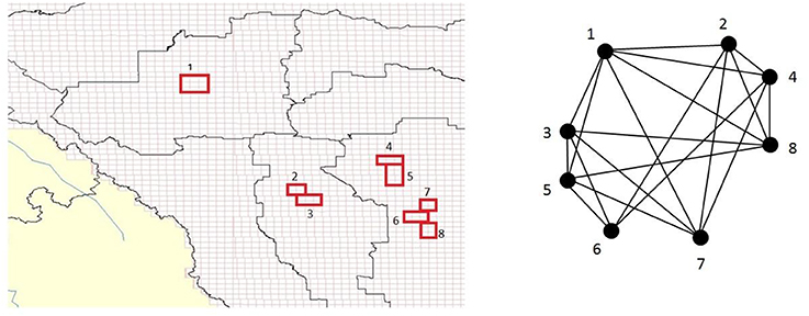
Figure 1. (Left) Hypothetical depiction associating subregions (red) within a complex spatio-temporal GIS environment/landscape to a constructed clique-based Bayesian causal network (BN) model with encoded dependence (Right). In this way, general BN virtual model representations could be designed for various intended applications (e.g., urban land-use, animal habitat suitability) and encoded linked with a given GIS study region/real-world environment. The BN can then be pruned to remove irrelevant variables, and updated based on new knowledge as it becomes available, with prior marginal clique probabilities computed via (maximal) clique tree propagation.

A BN with encoded spatial dependence, to satisfy the conditions necessary for its constituent conditional distributions, would require a valid joint distribution (i.e., strictly positive density) according to the Hammersley-Clifford (HT) Theorem (Hammersley and Clifford, Unpublished). A MRF is a random field superimposed on a graph or network structure (that may be cyclic), as an undirected graphical model (UGM) in which each node corresponds to a single or set of random variables, and its edges represent conditional probability dependencies. One can convert a DGM- to a decomposable UGM-type network by means of moralization to ensure conditional independence assumptions are satisfied. Finding a clique in an UGM is equivalent to a clique in a DGM, if edges between node pairs (u,v) are created iff (if and only if) there are directed edges u → v and v → u. Some distributions can be perfectly modeled by either type (so-called decomposable or chordal), while neither representation is more powerful than the other (Murphy, 2013). However, UGMs (e.g., MRFs) have no topological ordering, so the chain rule cannot be used to represent the joint distribution, and conditional probability distributions (CPDs) are associated with potential functions in maximal cliques in a graph, rather than with each node. According to the HT Theorem, Gaussian MRFs can be decomposed into a set of so-called neighborhood Gibbs probability measures, or potential functions, in maximal graph cliques (a maximal-clique is the largest possible complete subgraph where each pair of vertices are connected). A mixture or ensemble of models comprising mixtures of Gaussian CPDs, p, can be defined by the following log-linear form, involving a random variable z(s_i) across sites s_i (i = 1,…,n) within neighborhoods N_i for the i^th site can then be defined as (Cressie and Lele, 1992),

$\begin{array}{l}logp(z\left(s_i\right)|z\left(N_i\right))=G\left(z(s_i)\right)+\beta {\displaystyle \sum _{j ϵ N_i}z(s_i)z(s_j)}\\ -\kappa \left(\beta ,{\displaystyle \sum _{j ϵ N_i}z(s_i)}\right). & (7)\end{array}$

The first term G(z(s_i)) represents dominant features of random variation and the second term β ∑_{j ϵ Ni} z(s_i) z(s_j) specifies spatial dependence within a neighborhood N, where the parameter β measures spatial dependence strength and direction. The exponential of the third term (i.e., exp(-κ(,))) is the normalizing constant that ensures p is a probability density (i.e., integrates to 1). By choosing different G functions, different auto-models can be generated (e.g., assuming z is real-valued and continuous, then exp(G) can comprise a mixture of Gaussian densities; Cressie and Wikle, 2011).

Concluding Remarks

We have explored how such dependencies could be embedded into BN models, from the perspective of fundamental assumptions governing space-time dynamics, highlighting the potential benefits of decomposing or factorization of the joint probability distribution of a BN into potential functions with spatial dependence encoded (Zhang and Poole, 1994). Encoding spatial dependence facilitates predictive modeling of a BN's joint distribution across an entire geographic region of interest (with respect to potential functions computing based on network cliques) enabling network pruning irrelevant variables and accommodating changes to the knowledge base, but relies on clique tree propagation for precomputation prior marginal probability of each clique. Consequently, coupled BN-GIS models that do not generate a joint probability distribution across a full study domain are represented as a set of conditional distributions for individual sub-regions. Often these sub-regions are context-specific, being defined from attributes of a problem (e.g., availability of data, identifiable boundaries), rather than more complex notions of spatial and temporal dependence (e.g., memory, covariance etc.) within the context of model prediction. A more complete representation of spatial dependency, potentially provides greater methodological consistency in verification and validation of dependence modeling and decision-making assumptions (e.g., for monitoring and predicting resource use and allocation decisions within heterogeneous-structured urban and rural landscapes). There is also increasing interest both in cluster-based randomized controlled trials (RCTs) and partitioning ecosystems for sustainability, where randomization is carried out over geographic units such as defined “maximum network cliques” or resource competition “harvesting niches” (Donovan et al., 2012; White et al., 2014; Murray, 2016). This approach is particularly well-suited to integrating new monitoring technologies (sensor networks, drone and satellite remote-sensing), while also adding greater flexibility to the suite of sampling approaches (i.e., simple, matched-pair, stratified, quasi-experimental) available. Computationally, an encoded dependence approach facilitates BN-inference by means of clique tree clustering and propagation (i.e., clique tree growth as a function of parameters that can be computed in polynomial time from BNs; Mengshoel, 2010). This is a crucial aspect, as the inclusion of the spatial Markov property results in an Mth-order Markov chain, with M depending on the number of first order sub regions that border a given region. For square grid cells, M = 4 for Rook's contiguity and M = 8 for Queen's contiguity whereas for sub regions based on vector data (e.g., soil features, administrative features, agro-economic zones), M would vary according to the number of adjacent neighbors. Given that there are K^M−1(K − 1) parameters, it is preferable to use connectivity rules that keep M as low as possible but still capture spatial dependencies in the data (Bishop, 2011). A class of BN namely, Bayesian copula-based BNs, are attracting increasing interdisciplinary interest, and may offer great benefits for modeling non-Gaussian multivariate probability distributions in high-dimensional applications. This approach to encode spatial dependence via a copula function applied to a set of cumulative distribution functions involving the random variables could then be seamlessly integrated within GIS via a separation of geographic buffer and overlay, whereby categorical distance relationships define buffers, and transformed equations represent spatial overlays. Encoding spatial (and temporal) dependence into BNs through factorization of the joint probability distribution could increase their accuracy, reliability, and scalability for environmental risk prediction and decision analysis, particularly for those applications that involve their verification and validation within GIS computing environments.

Author Contributions

JS: Worked with DL and NN to review literature and implement spatial concepts in model formulation. Exchanged the Markov assumption with Spatial Markov assumption and extended temporal Bayes Net model formula to accommodate spatial concepts. NN: Evaluated the validity of the joint probability distribution under Spatially explicit Bayes net concept (incorporating the Spatial Markov assumption) in light of the Hammersley-Clifford Theorem. Synthesized JS model formulation within broader mathematical framework and explained impact for modeling environmental variables. Created Figure 1. DL: Identified the need to use other quantitative techniques than linear combinations to model environmental variables (agroecological) for yield estimation and other agronomically important activities as part of biofuels grant JS and DL were operating under. Conducted literature review with JS and helped determine that current implementations of Bayesian networks were not actually spatially explicit. Guided JS in implementing spatial concepts in model formulation, serving in an advisory capacity.

Conflict of Interest Statement

The authors declare that the research was conducted in the absence of any commercial or financial relationships that could be construed as a potential conflict of interest.

Acknowledgments

JS and DL were supported by Research Grant Award No. 2012-10008-19727 from the USDA National Institute of Food and Agriculture. NN was supported by Growing Forward 2 Program, Agriculture and Agri-Food Canada (AAFC). We thank Dr. T. A. Porcelli for editorial assistance.

References

Aalders, I. (2008). Modeling land-use decision behavior with Bayesian belief networks. Ecol. Soc. 13:16. doi: 10.5751/ES-02362-130116

CrossRef Full Text | Google Scholar

Aguilera, P. A., Fernández, A., Fernández, R., Rumí, R., and Salmerón, A. (2011). Bayesian networks in environmental modelling. Environ. Model. Softw. 26, 1376–1388. doi: 10.1016/j.envsoft.2011.06.004

CrossRef Full Text | Google Scholar

Bishop, C. M. (2011). Pattern Recognition and Machine Learning. New York, NY: Springer.

Google Scholar

Chen, S. H., and Pollino, C. A. (2012). Good practice in Bayesian network modelling. Environ. Model. Softw. 37, 134–145. doi: 10.1016/j.envsoft.2012.03.012

CrossRef Full Text | Google Scholar

Cressie, N., and Lele, S. (1992). New models for Markov random fields. J. Appl. Prob. 29, 877–884. doi: 10.1017/S0021900200043758

CrossRef Full Text | Google Scholar

Cressie, N., and Wikle, C. K. (2011). Statistics for Spatio-Temporal Data. Hoboken, NJ: John Wiley & Sons.

Google Scholar

Darwiche, A. (2010). Bayesian networks. Commun. ACM. 53, 80–90. doi: 10.1145/1859204.1859227

PubMed Abstract | CrossRef Full Text | Google Scholar

Dean, T., and Kazawa, K. (1989). A model for reasoning about persistence and causation. Comput. Intell. 5, 142–150. doi: 10.1111/j.1467-8640.1989.tb00324.x

CrossRef Full Text | Google Scholar

Donovan, T. M., Warrington, G. S., Schwenk, W. S., and Dinitz, J. H. (2012). Estimating landscape carrying capacity through maximum clique analysis. Ecol. Appl. 22, 2265–2276. doi: 10.1890/11-1804.1

PubMed Abstract | CrossRef Full Text | Google Scholar

Fenton, N., and Neil, M. (2013). Risk Assessment and Decision Analysis with Bayesian Networks. Boca Raton, FL: Taylor & Francis (Chapman & Hall/CRC Press).

Google Scholar

Goodchild, M. F. (1992). Geographical information science. Int. J. Geogr. Inf. Sci. 6, 31–45.

Google Scholar

Grêt-Regamey, A., Brunner, S. H., Altwegg, J., Christen, M., and Bebi, P. (2013). Integrating expert knowledge into mapping ecosystem services trade-offs for sustainable forest management. Ecol. Soc. 18:34. doi: 10.5751/es-05800-180334

CrossRef Full Text | Google Scholar

Grêt-Regamey, A., and Straub, D. (2006). Spatially explicit avalanche risk assessment linking Bayesian networks to a GIS. Nat. Hazard Earth Sys. 6, 911–926. doi: 10.5194/nhess-6-911-2006

CrossRef Full Text | Google Scholar

Izenman, A. J. (2013). Modern Multivariate Statistical Techniques: Regression, Classification, and Manifold Learning, 2nd Edn. New York, NY: Springer.

Google Scholar

Kim, S. K., Lee, J. H., Ryu, K. H., and Kim, U. (2014). A framework of spatial co-location pattern mining for ubiquitous GIS. Multimed. Tools Appl. 71, 199–218. doi: 10.1007/s11042-012-1007-2

CrossRef Full Text | Google Scholar

Koller, D., and Friedman, N. (2009). Probabilistic Graphical Models: Principles and Techniques. Cambridge: MIT Press.

Google Scholar

Liu, U., Gupta, H., Springer, E., and Wagener, T. (2008). Linking science with environmental decision making: experiences from an integrated modeling approach to supporting sustainable water resources management. Env. Model. Sofw. 23, 846–858. doi: 10.1016/j.envsoft.2007.10.007

CrossRef Full Text | Google Scholar

Liu, Y., Feng, X., Wang, Q., Zhang, H., and Wang, X. (2014). Prediction of urban road congestion using a Bayesian network approach. Proc. Soc. Behav. Sci. 138, 671–678. doi: 10.1016/j.sbspro.2014.07.259

CrossRef Full Text | Google Scholar

Mengshoel, O. J. (2010). Understanding the scalability of Bayesian network inference using clique tree growth curves. Artif. Intell. 174, 984–1006. doi: 10.1016/j.artint.2010.05.007

CrossRef Full Text | Google Scholar

Meyer, S. R., Johnson, M. L., Lilieholm, R. J., and Cronan, C. S. (2014). Development of a stakeholder-driven spatial modeling framework for strategic landscape planning using Bayesian networks across two urban-rural gradients in Maine, USA. Ecol. Model. 291, 42–57. doi: 10.1016/j.ecolmodel.2014.06.023

CrossRef Full Text | Google Scholar

Murphy, K. P. (2013). Machine Learning: A Probabilistic Perspective. Adaptive Computation and Machine Learning Series, 4th Edn. Cambridge, MA: MIT Press.

Murray, M. G. (2016). Partitioning ecosystems for sustainability. Ecol. Appl. 26, 624–636. doi: 10.1890/14-1156

PubMed Abstract | CrossRef Full Text | Google Scholar

Newlands, N. K. (2016). Future Sustainable Ecosystems: Complexity, Risk, Uncertainty. Boca Raton, FL: Taylor & Francis (Chapman & Hall/CRC). Applied Environmental Statistics Series.

Google Scholar

Rozanov, J. A. (1977). Markov random fields and stochastic partial differential equations. Math. USSR Sbornik 32, 515–534. doi: 10.1070/SM1977v032n04ABEH002404

CrossRef Full Text | Google Scholar

Simpson, D., Lindgren, F., and Rue, H. (2012). Think continuous: Markovian Gaussian models in spatial statistics. Spatial Stat. 1, 16–29. doi: 10.1016/j.spasta.2012.02.003

CrossRef Full Text | Google Scholar

White, H., Sabarwal, S., and de Hoop, T. (2014). Randomized Controlled Trials (RCTs). Methodological Briefs, Impact Evaluation No. 7. Florence: United Nations Children's Fund (UNICEF) Office of Research.

Zhang, N. L., and Poole, D. (1994). “A simple approach to Bayesian network computations,” in Proceedings of the 10th Canadian Artificial Intelligence Conference (AI-94) (Banff), 171–178.