Discrete-Continuum Multiphase Model for Structure Formation in Soils Including Electrostatic Effects

1. Introduction

Understanding the structural formation in soils with respect to space and time is highly demanding at any scale. Pedogenesis induces an aggregate structure in most soils (see Totsche et al., 2018), and hierarchical concepts have been developed for it (c.f. Tisdall and Oades, 1982; Six et al., 2000, 2004; Totsche et al., 2018). We concentrate on the smallest building units that form the so-called microaggregates, which typically have a diameter of <250 microns (Totsche et al., 2018). In their reviews Six et al. (2004) and Totsche et al. (2018) point out that a quantification of the dynamic interrelation between the major influencing factors for microaggregate formation is clearly necessary. This lack of quantifying studies may be due to the manifold of interactions, the different scales on which the mechanisms operate, and the heterogeneity of the porous system (Six et al., 2004). Thus, detailed, process-driven models going down to the scale of microaggregates are rare. Recently, new experimental techniques allow to investigate these scales (c.f. Totsche et al., 2018), and porescale geometries of natural soils may be imaged with reasonable high resolution. However, also advanced imaging techniques are still often restricted to a static view such that the dynamics of aggregation mechanisms are poorly understood up to now. Dynamic measurements and obtained insights push forward mechanistic models describing the dynamic aggregation processes. An operative tool based on mechanistic principles that allows to study in silico the formation of such aggregates thus could be helpful to supplement experiments, and also provide a link to soil functions like water retention curves.

However, to our knowledge no currently available model is able to simulate a fully dynamic and mechanistic evolution of the soil structure. A first step towards that direction applying cellular automaton methods (CAMs) has been made in the work of Crawford et al. (2012) (see also the references cited therein), and Ray et al. (2017).

CAMs provide a flexible way to describe the restructuring of soil particles and pore-filling phases. The variability in soil structure as a consequence of the self organization of the soil-microbe system has been investigated in Crawford et al. (2012). Extracellular polymeric substances (termed gluing agents in Totsche et al., 2018) are emerging which enhance the binding of soil particles.

CAMs have also been applied in the context of biofilm models. In combination with experiments, Tang and coworkers prescribed biomass spreading rules in Tang and Valocchi (2013) and Tang et al. (2013), and investigated the structural development of biofilm at the pore scale. Likewise, the coupling of a cellular automaton model for biofilm growth to fluid flow and solute transport is considered in Benioug et al. (2017) and its impact on the hydraulic conductivity is studied.

In Ray et al. (2017) both aforementioned processes were combined in a comprehensive pore-scale model that allows to study the interplay of solutes, bacteria, biomass, and solid particles. It is based on a combined partial differential equation (PDE) model and cellular automaton formulation. However, further important processes and mechanisms need to be included to study their influence on structure formation, and for accessing more realistic applications. In addition to microbial activity and biofilm development microaggregate formation strongly depends on the characteristic properties of the system such as saturation and of its constituents including particle shape or charge (c.f. Totsche et al., 2018). Moreover, the break-up of aggregates due to the interplay of attractive and repulsive forces has to be taken into account for a reasonable aggregation model.

In this research, we present the related model extensions and study their impact using simulation scenarios. The CAM rules are adapted for the effects of solid surface charges and ion transport, and their impact is considered also in the solute. Rotations of solid particles are for instance included into the model to facilitate the aggregation of solid particles with opposite face charges.

To study the formation of microaggregates from building units of diverse types new prototypes have been implemented to represent different geometric structures. Moreover, a gas phase has been included to consider moisture variations. Thus situations can be taken into account where the aggregates are not fully saturated but, e.g., coated only by a thin film of water. A restructuring of the solid phase may then induce the necessity of a reorganization of the gas phase to maintain the non-wetting properties (section 2.3.2). Exchange between and transport within the different phases may become prominent since mobility of species varies within water, gas, or biofilm. As electric forces are an important driving force for aggregation—as highlighted in Totsche et al. (2018)—the Nernst-Planck-Poisson equations are applied to determine the movement of ions. We furthermore consider homogeneous chemical reactions (e.g., described via the mass action law) within the fluid phases and biofilm, as well as heterogeneous reactions with the solid phase.

Several simulation scenarios are investigated in two dimensions to demonstrate the effects of the novel mechanisms. The underlying model equations are discretized by means of a local discontinuous Galerkin (LDG) method as presented and analyzed in Rupp and Knabner (2017), Aizinger et al. (2018), and Rupp et al. (2018) and solved globally fully implicitly using an implementation in M++ (Wieners, 2005). The results are discussed thoroughly focusing on the influencing conditions for structure formation. Along this line, we emphasize the emergence of phenomena observed in soils such as the creation of cardhouse structures under the presence of charges, the occurrence of liquid bridges (Carminati et al., 2017) under unsaturated conditions, or the characterization of regions with high or low nutrient availability.

The paper is structured as follows: In section 2, we establish the underlying mathematical model. We shortly review the model introduced in Ray et al. (2017) and thoroughly discuss its extensions. Section 2.5 mentions the used numerical methods and describes the overall algorithm. In section 3 the presented model is investigated numerically. With several simulation scenarios we illuminate the role of shapes and charges. Section 4 wraps up the manuscript by summarizing the results.

2. Materials and Methods—Geometry and Mathematical Model

2.1. Model Parts

Within our model, we essentially consider the following prototypical time- and space-dependent model parts:

1. a solid phase (s). A gluing agent may be present on the solid surfaces, and also (variable) surface charges which influence the restructuring rules. Additionally, heterogeneous reactions with mobile chemical species may take place on the solid surfaces.

2. a fluid phase (f), the wetting phase, in which potentially charged chemical species diffuse and react.

3. a bio phase (b) in which potentially charged chemical species react and diffuse with lower diffusivity and mobility than in the fluid. Moreover, biomass development is treated as described in Ray et al. (2017).

4. a gas phase (g), the non-wetting phase, in which reacting chemical species diffuse with the highest diffusivity.

5. several types of mobile, potentially charged chemical species that may participate in heterogeneous or homogeneous reactions. Species that are present in the gas and the fluid/bio phase follow Henry's Law as transfer condition. Examples for relevant chemical species are for instance oxygen, or nitrate as nutrients for bacteria and microorganisms creating extracellular polymeric substances (EPS) and biomass.

6. a gluing agent (e.g., EPS) which is produced as a consequence of local biological activity (c.f. Crawford et al., 2012; Ray et al., 2017).

2.2. Discrete Geometry

The cellular automaton acts on a regular quadrilateral domain Y with periodic boundary ∂Y (dashed lines in Figure 1) being covered by a regular grid containing N² squares Yⁱ with faces ∂Yⁱ. At first, one of the following cell states is (randomly, but in desired proportions) assigned to each of the squares: “bio” (b), “fluid” (f), “solid” (s), or “gas” (g) (c.f. Figure 1). Note that this is distinct from real world situations, where the fluid distribution depends for instance on wettability and pore sizes. However, we want to emphasize the self-organization of the system due to the underlying mechanisms without relying on specific spatial structures. The additional consideration of more realistic structures, e.g., as a result of CT images, is focus of forthcoming research.

FIGURE 1

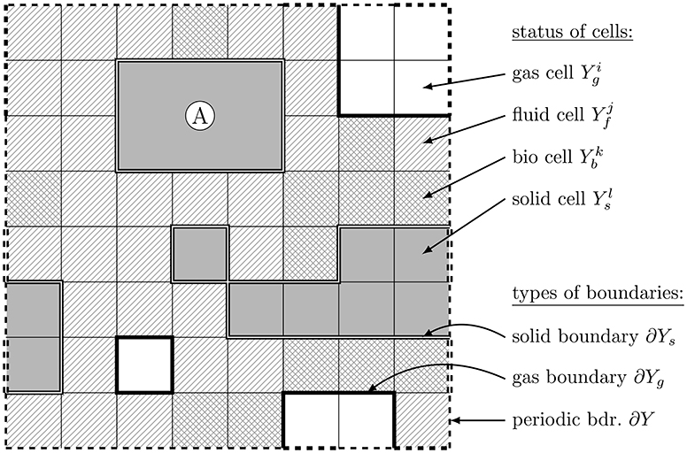
Figure 1. Domain Y, geometric structure, cell states—gas ( ), fluid (), bio (), solid ()—and prototypic representation of an inseparable building unit Ⓐ.

The cells Yⁱ in the cellular automaton correspond to the smallest physical units in the model. In our new approach different inseparable building units with various shapes may be defined that are composed of cells Yⁱ (c.f. Figure 2). We thus can consider for instance (approximately) spherical geometries, needle shapes, or plates, and investigate the interaction of these structures and the resulting soil structures. The inseparable building units may represent prototypes of e.g., quartz, goethite, or illite particles (c.f. Figure 2 or Ⓐ in Figure 1). Additionally, composites of different building units may be considered (c.f. Figure 2).

FIGURE 2

Figure 2. Possible shapes of building units (size not to scale); from left to right: Spherical, platy, or needle-like, and composites. Black and white to indicate equal charge for the composites.

The union ${\bigcup }_i{Y}_s^i$ of all solid cells is termed the solid phase and denoted by Y_s with boundary Γ: = ∂Y_s. Likewise, the union ${\bigcup }_i{Y}_b^i$ of all bio cells—the bio phase—is denoted by Y_b, the union ${\bigcup }_i{Y}_f^i$ of all fluid cells—the fluid phase—by Y_f, and the union ${\bigcup }_i{Y}_g^i$ of all gas cells—the gas phase—by Y_g (c.f. Figure 1). Furthermore, we denote the union of fluid and bio phase with liquid phase and define the interface Γ_LG: = (∂(Y_f ∪ Y_b)) ∩ ∂ Y_g of the gas with the liquid phase. In each time step a redistribution of the respective phases is defined according to restructuring / growing and shrinking / reorganizing rules in the cellular automaton framework (c.f. Ray et al., 2017 and section 2.3).

Within the fluid, bio, and gas phases, the continuum parts of the model come into play. Here, (possibly coupled, partial) differential equations are solved for the transported, potentially charged chemical species, and also the immobile biomass. Likewise, an ordinary differential equation is considered for the gluing agent (e.g., EPS), possibly being present on ${\bigcup }_i\partial Y_s^i\cup {\bigcup }_i\partial Y_b^i$ and holding together bio and/or solid cells. A detailed statement of the ordinary differential equation describing the oxygen-dependent growth and decay of gluing agent, which lives on the boundaries of bio and solid cells, can be found in Ray et al. (2017). The extensions of the model are discussed in the following.

2.3. Cellular Automaton Method (CAM)

The cellular automaton rules are based on the movement of the building units (section 2.2). For single cells this was already described in Ray et al. (2017). Building units that are not bound to either biomass or further solids by either gluing agent or electric forces have the ability to move. For the ease of presentation we describe the CAM rules for single cells, since an extension of the rules to inseparable building units or their composites is straightforward. The potential movement of cells in the cellular automaton method is always based on the evaluation of stencils (c.f. Figure 3), i.e., the investigation of the properties of neighboring cells. The stencil represents the range of influence of cells on each other. Within this research, stencils of different sizes up to 3 unit lengths [L] are considered.

FIGURE 3

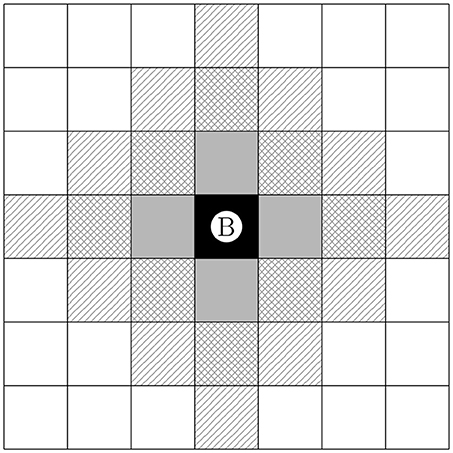
Figure 3. Stencil of size 0 () , 1 (), 2 (), and 3 () for the center cell Ⓑ.

2.3.1. CAM for Bio and Solid Phases

The application of the cellular automaton method was already discussed in Ray et al. (2017) for biomass development and solid restructuring. We briefly recapitulate the main issues:

The biomass spreading rule is based on the CAM described in Tang and Valocchi (2013) and Tang et al. (2013). In each time step, for all biomass cells $Y_b^i$ it is examined whether the mean biomass concentration exceeds a certain threshold value. Then, the neighboring fluid cells are tested whether they may take up a certain amount of excess biomass. In doing so, a shortest path strategy is applied.

The CAM rules for uncharged solid cells are inspired by Crawford et al. (2012) and described in detail in Ray et al. (2017). In our new model, we likewise consider inseparable building units or their composites for which the CAM rules are defined analogously. Additionally, we account for electrostatic effects and the resulting reorganization of the solid due to charges. The respective CAM rules are superimposed with the rules described in Ray et al. (2017) as shown in Equation (2).

For the new CAM, “movable cells” $Y_s^{î}$ are identified first. Note that with the gluing agent concentration possibly decaying in time, composites may break up again. The break up particularly happens if electrostatic repulsion becomes predominant in comparison to the gluing properties. The counterbalance of electric forces and gluing properties on common faces of neighboring solid cells $Y_s^k$ is evaluated in the following expression:

$\begin{array}{cc}{c}_{\alpha ,\widehat{i}k}-\tilde{\gamma }{\displaystyle {\int }_{\partial Y_s^{\widehat{i}}\cap \partial Y_s^k}{\rho }_e^{\Gamma ,Y_s^{\widehat{i}}}}{\rho }_e^{\Gamma ,Y_s^k}\le 0.& (1)\end{array}$

Here, c_{α, îk} [1/L] denotes the average concentration of the gluing agent at the common face of the neighboring solid cells $Y_s^{î}$ and $Y_s^k$. Likewise, ${\rho }_e^{\Gamma ,Y_s^{î}}$ [IT/L] and ${\rho }_e^{\Gamma ,Y_s^k}$ [IT/L] denote the surface charge densities at the common face of the neighboring solid cells $Y_s^{î}$ and $Y_s^k$. [L] is the unit for a length, [T] for time, [I] for the electric current measured in ampere, and later on we also use [M] for mass. Note that attraction means a positive contribution to the left-hand side of Equation (1) by gluing agent concentration or electric forces stemming from charge densities with opposite sign. On the other hand, electric repulsion means negative contribution from the second term for charge densities with like sign. The proportionality constant $\tilde{\gamma }>0$ [1/(IT)²] balances the impact of gluing and electric forces. If (1) holds true for all neighbors of $Y_s^{î}$, $Y_s^{î}$ is a cell with the ability to move in the CAM.

The attraction or affinity A_i [−] of potential target fluid or gas cells Yⁱ is then a weighted superposition of the different attracting forces related to gluing agent, type of neighbors, and electric forces:

$\begin{array}{cc}\begin{array}{l}{A}_i=\widehat{\gamma }\left({\displaystyle \sum _{\begin{array}{c}\text{neighbors}\\ Y_s^{\widehat{i}}\ne Y^j\text{of}{Y}^i\end{array}}{c}_{\alpha ,ij}}\right)+\text{number of solid neighbors}\ne Y_{\text{s}}^{\widehat{\text{i}}}\text{ of }{Y}^i\\ -\overline{\gamma }\min \left\{\text{}{\displaystyle \sum _{\begin{array}{c}\text{neighbors}\\ Y_s^{\widehat{i}}\ne Y_s^j\text{of}{Y}^i\end{array}}\text{}}\text{}{\displaystyle {\int }_{\partial {\overline{Y}}_s^{\widehat{i}}\cap \partial Y_s^j}{\rho }_e^{\Gamma ,{\overline{Y}}_s^{\widehat{i}}}}{\rho }_e^{\Gamma ,Y_s^j}d\sigma |{\overline{Y}}_{\text{s}}^{\widehat{\text{i}}}\text{ is a rotation of }{Y}_{\text{s}}^{\widehat{i}}\right\}\end{array}& (2)\end{array}$

with proportional constants $\widehat{\gamma }$ [L], $\bar{\gamma }$ [L/(IT)²], and i denoting the index of a cell contained in the stencil around the center cell (c.f. Figure 3). We emphasize that rotations of solid cells relative to each other may become prominent in the case that their faces are not equally charged. With our definition, we enable a reorganization into such favorable positions (c.f. Ⓒ in Figure 4).

FIGURE 4

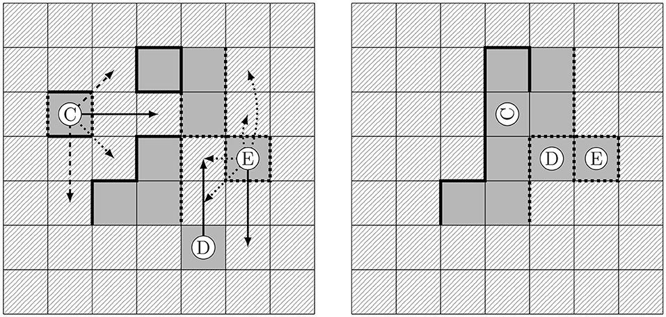
Figure 4. Effects of charges in solid restructuring. Initial configuration with potential movements to target cells for a stencil of 2 (left) and consolidated configuration following the strongest attraction for each particle (right). Straight and broken lines indicate opposite charges at the faces of the solid particles.

As in the case without charges, the target cell with the largest A_i is selected. If several target cells are identified as equally attractive, one is randomly chosen and the restructuring is carried out. A conflict may occur if the same target cell is selected by different mobile solid cells. To resolve such conflicts one solid cell is randomly chosen to move for each of the conflicts.

In Figure 4, we illustrate the reorganization of a charged solid phase. A stencil of width two, c.f. Figure 3, is applied to all solid cells. The arrows on the left hand side in Figure 4 indicate potential target cells for such a stencil. The continuous arrows indicate the jump to the most favorable positions for the respective cell. Dashed arrows indicate further possible and advantageous movements, while dotted arrows indicate disadvantageous configurations. On the right hand side in Figure 4 the final consolidated configuration is shown, after the cells have moved in alphabetical order. The effect of charges is clearly visible: The solid cell denoted with Ⓒ rotates in such a way that faces with opposite charges attach to one another and their charges balance out. Along this line the absolute net charge of the system decreases, while electroneutrality is preserved. The uncharged solid cell Ⓓ moves in such a way that it obtains the maximal possible number of neighboring solid cells. Afterwards, the optimal position for Ⓔ is its current position, since likely charged cells repel each other.

2.3.2. CAM for Gas Phase

In the following, we briefly discuss the extensions of the CAM due to the occurrence of a gas phase.

In natural soils the liquid (fluid and bio) phase is the wetting phase, while the gas phase is the non-wetting phase. In the cellular automaton rules this is implemented as follows: Whenever, a gas cell has a common interface with a solid cell, its direct neighbors are considered, i.e., a stencil of size 1 is applied (c.f. Figure 3). If there is only one liquid neighbor of the gas cell (like it is for Ⓖ in Figure 5), the gas cell and the liquid cell switch places. If there are several fluid/bio cells who are neighbors of the gas cell, one of the fluid/bio cells with the minimum amount of common interfaces with the solid phase is chosen to switch places with the gas cell. According to this rule fluid and bio cells attach to solid cells while gas cells do not. If the same target cell is selected by different gas cells, again one gas cell is randomly chosen to jump to the respective target cell and the possible reorganization of the remaining gas cells is postponed to subsequent iterations.

FIGURE 5

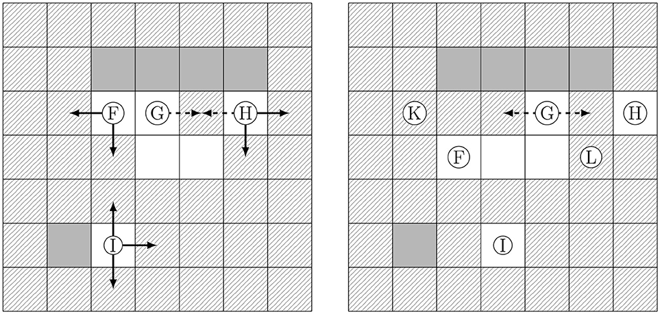
Figure 5. Reorganization of gas cells being tangent to solid cells. (Left) Favorable options (continuous arrows) leading to a loss of contact to solid, and further options (dashed arrows) having the same contact to solid. (Right) The cells Ⓕ Ⓗ, Ⓘ performed a favorable step, and Ⓖ moved also (dashed step). Ⓖ will repeatedly change positions tangent to the solid (equally favorable, dashed steps) until finally position Ⓚ or Ⓛ can be reached (by a favorable step).

In Figure 6 the functionality of the CAM is illustrated with focus on the reorganization of the gas phase and its non-wetting property on a computational domain consisting of 64 × 64 cells. A random configuration of solid (black), fluid (gray), and gas (white) cells with a volume proportion of 33% each is taken as starting point. After the CAM is run it is evident that the fluid forms a film on the consolidated solid phase, and even liquid bridges can be found as a result of the restructuring algorithm. Contrarily, the gas phase clearly shows its non-wetting property.

FIGURE 6

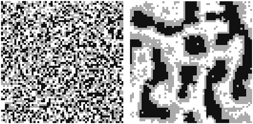
Figure 6. CAM including the reorganization of the gas phase illustrating its non-wetting property. Random initial configuration (left) and quasi stationary consolidated configuration (right) with solid (black), gas (white), and fluid (gray).

2.4. Nernst-Planck Equations for Ion Movement

The nonlinearly coupled Nernst-Planck-Poisson Equations (3) describe the movement of a potentially charged chemical species in the liquid, i.e., the time-dependent domain Y_f ∪ Y_b whose structural arrangement is defined in each time step by the CAM (see section 2.3). In contrast to this, the Poisson Equation (5) is defined on the whole periodic domain Y. In the following, ${\omega }_r^{\pm }$ [1/L²] denotes the volume concentrations of the r-th species and ${\omega }_r^{\Gamma ,\pm }$ [1/L] its surface concentration on the solid phase's boundary Γ: = ∂Y_s.

$\begin{array}{cc}{\partial }_t{\omega }_r^{\pm }\pm \nabla ·\left(C_r{\omega }_r^{\pm }\text{E}\right)-\nabla ·\left(D_r\nabla {\omega }_r^{\pm }\right)=R_r(\omega )\text{ in }(0,T)\times Y_f\cup Y_b,& (\mathrm{3a})\end{array}$

$\begin{array}{cc}k\left(g({\omega }_r^{\pm })-{\omega }_r^{\Gamma ,\pm }\right)={\partial }_t{\omega }_r^{\Gamma ,\pm }\text{ on }(0,T)\times \Gamma ,& (\mathrm{3b})\end{array}$

$\begin{array}{cc}\pm \left(C_r{\omega }_r^{\pm }\text{E}\right)·\nu -\left(D_r\nabla {\omega }_r^{\pm }\right)·\nu ={\partial }_t{\omega }_r^{\Gamma ,\pm }\text{ on }(0,T)\times \Gamma ,& (\mathrm{3c})\end{array}$

$\begin{array}{cc}\pm \left(C_r{\omega }_r^{\pm }\text{E}\right)·\nu -\left(D_r\nabla {\omega }_r^{\pm }\right)·\nu =0\text{ on }(0,T)\times ,& (\mathrm{3d})\end{array}$

$\begin{array}{cc}{\omega }_r^{\pm }={\omega }_{r,0}^{\pm }\text{ in}\left\{0\right\}\times Y_f\cup Y_b.& (3e)\end{array}$

Here, the advective flux is proportional to the electric field E [ML/(IT³)] with discontinuous, phase-dependent mobility C_r [IT²/M]. Likewise, the diffusivities D_r [L²/T] are discontinuous. The homogeneous reaction rates are denoted by R_r [1/(L² T)] and obey the mass action law while the heterogeneous reactions are described by the kinetic form of the Langmuir isotherm g(·) [1/L] with rate constant k [1/T](c.f. Sparks, 1989). Assuming that the domain evolves quite slowly (in the range of μm per day as can be deduced from Tang et al., 2013 where two discrete steps per day are chosen) compared to the speed of diffusion and reactions, the boundary condition represents balance of mass/charges while possible surface diffusion is neglected.

Since the mobility C_r vanishes for uncharged species ${\omega }_r^0$, reaction-diffusion equations are obtained which are similar to the ones considered in Ray et al. (2017). In this manuscript we additionally consider diffusion and reaction of uncharged species in the gas phase under appropriate initial conditions [c.f. (4)]. Moreover, we account for a possible phase transition of the uncharged species into the gas phase. At thermodynamical equilibrium and for dilute solutions (3d) is then replaced by Henry's law (4b) for these species:

$\begin{array}{cc}{\partial }_t{\omega }_r^0-\nabla ·\left(D_r\nabla {\omega }_r^0\right)=R_r(\omega )\text{\hspace{1em}in }(0,T)\times Y_g,& (\mathrm{4a})\end{array}$

$\begin{array}{cc}{\omega }_r^0{|}_{Y_g}/{\omega }_r^0{|}_{Y_f\cup Y_b}=H_r^{\Gamma }{}^{\text{LG}}\text{\hspace{1em}on }(0,T)\times {\Gamma }_{\text{LG}},& (\mathrm{4b})\end{array}$

$\begin{array}{cc}{\left(D_r\nabla {\omega }_r^0\right)|}_{Y_g}·{\nu }_g={\left(D_r\nabla {\omega }_r^0\right)|}_{Y_f\cup Y_b}·{\nu }_g\text{ on }(0,T)\times {\Gamma }_{\text{LG}}& (\mathrm{4c})\end{array}$

$\begin{array}{cc}-\left(D_r\nabla {\omega }_r^0\right)·\nu =0\text{\hspace{1em}on }(0,T)\times \Gamma ,& (\mathrm{4d})\end{array}$

$\begin{array}{cc}{\omega }_r^0={\omega }_{r,0}^0\text{\hspace{1em}in }\left\{0\right\}\times Y_g& (4e)\end{array}$

with the inverse solubility constant of Henry's law $H_r^{\Gamma \mathrm{\text{LG}}}$ [−].

The electric field E and the electric potential Φ [ML²/(T³I)] are computed in terms of a Poisson equation with sub-dimensional sources ${\rho }_e^{{\Gamma }^s}$ (since these source terms are defined on the d − 1-dimensional boundaries of the solids):

$\begin{array}{cc}-\nabla ·\left({ϵ}_0{ϵ}_r\nabla \Phi \right)={\rho }_e+\vartheta {\rho }_e^{{\Gamma }^s}\text{ in }(0,T)\times Y,& (\mathrm{5a})\end{array}$

$\begin{array}{cc}\text{E}=-\nabla \Phi \text{ in }(0,T)\times Y,& (\mathrm{5b})\end{array}$

$\begin{array}{cc}{\displaystyle {\int }_Y\Phi }d\text{x}=0\text{ in }(0,T),& (\mathrm{5c})\end{array}$

where ${\rho }_e=\sum _{r=1}^N{z}_{r}e{\omega }_r^{\pm }$ [IT/L²] and ${\rho }_e^{{\Gamma }^s}=\sum _{r=1}^N{z}_{r}e{\omega }_r^{\Gamma ,\pm }$ [IT/L] denote the charge densities in the fluid and on the solid cells' boundaries ${\Gamma }^s:={\bigcup }_i\partial Y_s^i$, respectively, and scaling factor ϑ = 1 [L^-1]. Finally, e is the elementary charge [IT] and z_r [−] is the charge number of the r-th species, ϵ₀ [I²T⁴/(ML²)] denotes the dielectric permittivity, and ϵ_r [−] is the discontinuous, phase depending relative dielectric permittivity.

The consistency condition

${\displaystyle {\int }_Y{\rho }_e}d\text{x}=-{\displaystyle {\int }_{{\Gamma }^s}{\rho }_e^{{\Gamma }^s}d\text{σ}},$

complements the model meaning that sources and sinks of the electric potential cancel out globally, i.e., the whole domain must be electrically neutral. Hence, R_r cannot be chosen randomly but has to ensure the conservation of charge, while g can be an arbitrary boundary reaction, as the flux-boundary condition in (3c) ensures conservation of charge independently of g. Moreover, the initial condition (3e) has to be consistent with the electroneutrality condition.

2.5. Numerical Methods

The equations of the continuum model part (3), (4), (5) are discretized using the local discontinuous Galerkin method as described in Rupp and Knabner (2017) and Rupp et al. (2018) on the grid composed of squares which is naturally induced by the model formulation (c.f. Figure 1). The lower dimensional source terms are incorporated as symmetric flux corrections. The used discretization of Henry's law can be found in Rupp et al. (2018). Finally, the fully discrete system of equations is obtained via an approximation of the time-derivative by the first order backward difference quotient, i.e., we apply an adaptive, implicit Euler scheme. To ensure the local convergence of Newton's method applied to the nonlinear set of Nernst-Planck equations restrictions of the time step may be necessary. Note that unlike the algorithm in [Ray et al., 2017, subsection 2.5 (Table 2)], we solve the complete resulting non-linear system of equations (NLSE) here fully implicitly with Newton's method.

The overall algorithm including the continuum model part and the discrete CAM is depicted in Table 1, where t [T] is the old time step, τ [T] denotes the time step size, $\tilde{t}$ [T] is the current time when the CAM is evaluated, T [T] is the end time of the simulation, and MAXITER [−], ϵ₁ [−], ϵ₂ [−] are constants. The frequency of updates of the geometric structure (defined by $\tilde{\tau }$ [T]) has an important impact on the evolution of the domain and thus has to be related with realistic time intervals in an non-artificial simulation. In Tang et al. (2013) twice a day is chosen. A second time stepping (t, τ) is introduced for operator splitting between the different types of models in section 2.4, but in numerical experiments we most often recognized that $\tau =\tilde{\tau }$ yields good results.

TABLE 1

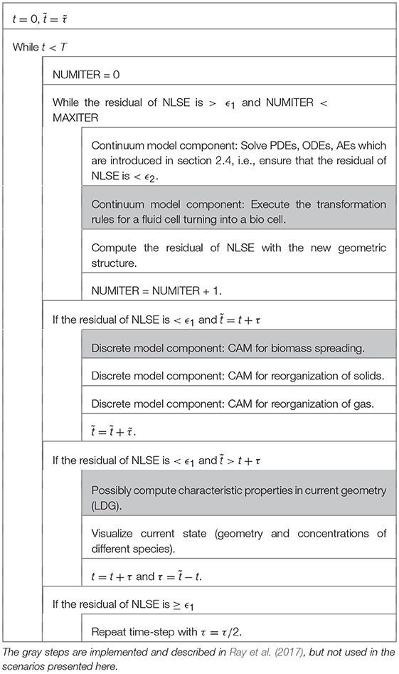
Table 1. Algorithm for discrete-continuum model.

Within the discrete model part—which is solved for all global time steps—the main factors related to structural changes, apart from the generation of biomass from bacteria, are evaluated, namely the biomass spreading, solid restructuring and reorganization of the gas phase. The implementation is written in C++ and based on M++ (Wieners, 2005) and uses MPI parallelization for the PDE and the CAM parts of the model. The CAM part of the model induces a lot of communication between different processors (especially for larger stencils). Conflict resolution strategies have to be incorporated if different cells have the same target location and jumps over processors' boundaries are necessary. In general, we recognized that the computational effort of the CAM increases drastically (compared to the effort for solving the PDEs) if the portion of solid is high and large stencils are applied.

3. Results and Discussion—Simulation Scenarios

To demonstrate the impact of the implemented mechanisms on the formation of structures in soils, we present several simulation scenarios. The first scenarios focus on the demonstration of single effects and are chosen in such a way that the self organization according to CAM rules is illustrated. To this end, various model components such as charges, biomass, gluing agent, or solutes in the liquid etc. are switched off. Thereafter, combined effects are investigated to illustrate the overall capability of the model. Finally, the interplay of the discrete and continuum model component is shown.

3.1. Effect of the Range of Attraction

First, we investigate the influence of the range of attraction of particles on each other for structure formation which is represented by different stencil widths. Since this scenario focuses on the demonstration of a single effect, no charges, biomass, gluing agent, or solutes in the liquid etc. are taken into account. Thus, attraction of the cells to each other is uniform and can be interpreted as the sum of attracting forces as, e.g., van der Waals forces, that lead also to homoaggregation. It is thus only determined by the number of neighbors [see Equation (2) with $\widehat{\gamma }=\bar{\gamma }=0$]. Initially, a domain with 50% solid cells and 50% fluid cells and 256 × 256 cells in total is randomly created and any charge effects are disregarded. From this initial configuration (c.f. picture on the left in Figure 7) the CAM is run with a stencil of width 1 [L] and with a stencil of width 3 [L] (c.f. Figure 3).

FIGURE 7

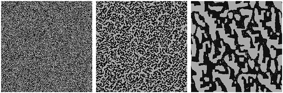
Figure 7. Self organization depending on range of attraction: (Left) Initial, random configuration of single solid cells (black) with porosity θ = 0.5; (Middle) quasi-stationary state with stencil 1, (Right) quasi-stationary state with stencil 3.

Since we study the formation of structures and do not consider their disaggregation here, the simulations run into a quasi-stationary state. The resulting aggregated structures are depicted in the middle of Figure 7 (for a stencil of width 1) and in the right of Figure 7 (for a stencil of width 3). It is evident that the self organization of the solid phase highly depends on the range of attraction represented by the size of the stencil. A smaller range of attraction leads to finer structures, i.e., higher specific surface areas of the solid phase (initially: 65, 168/32, 768 ≈ 1.99 [L^-1], stencil of size 1: 29, 720/32, 768 ≈ 0.91 [L^-1], stencil of size 3: 9, 208/32, 768 ≈ 0.28 [L^-1] after 500 CAM steps; Figure 7). Contrarily, the larger range of attraction induces coarser, connected structures, and thus also the average size of the pore channels is larger (Figure 7, right). Although the choice of the stencil width representing the range of electric forces can be determined quite well (see Liang et al., 2007), the analog of the attraction range originating from other forces such as gluing effects, has to be estimated. Our model allows to study such effects separately to validate related assumptions. Moreover, the combination of different effects on structure formation may also be studied in silico. In principle, each prototype of particle (c.f. Figure 2) may have a different range of attraction depending for instance on its charge. This is represented in the model as an individual stencil size (see Figure 3) for each prototype of a particle.

3.2. Effect of the Shape of Building Units

The shape and size of the inseparable building units strongly influence the formation of structural patterns. For an illustration of this effect, we consider domains of sizes 256 × 256 cells where 50% are filled by uncharged solid particles (either single cells or needles of length 5). In Figure 8 the random initial configurations are shown on the left hand side. The corresponding quasi-stationary states (after 500 CAM steps) are depicted on the right hand side. Note that the first line of Figure 8 is included in Figure 7. For each simulation a stencil of size 1 is applied. It is evident that rearrangement and aggregation have occurred for both simulation scenarios which are, however, more prominent in case of the single cells. This is clearly due to size effects since the rearrangement of needles is physically restricted for quite high volume fractions of the solid. The small building units have more options to move to a free single cell, and thus create denser structures. So less smooth structures are created for the needles as compared to the single cells and the surface has decreased less: for the the latter ones by a factor of 0.46 (from initially 1.99 to 0.91 [L^-1]), and for the needles by a factor of 0.84 (from 46, 096/32, 768 ≈ 1.41 to 38, 950/32, 768 ≈ 1.19 [L^-1]).

FIGURE 8

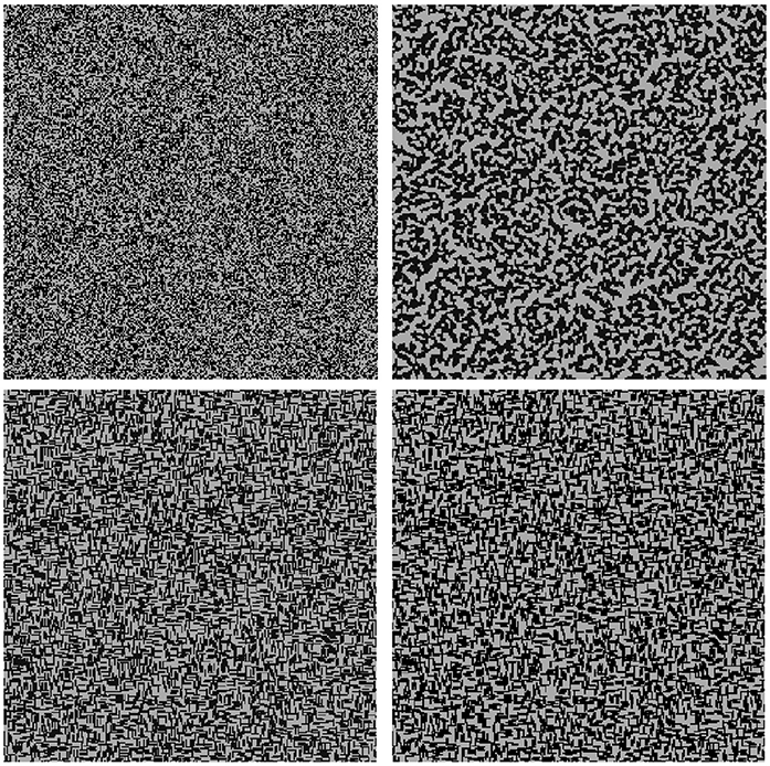
Figure 8. Self organization depending on shape and size constraints: (Left) Initial random configuration with single solid cells (top) and needles (bottom) in black with porosity θ = 0.5; (Right) Quasi-stationary states with a stencil of 1.

3.3. Effect of Charges

Electrostatic forces are a major driving force for particle aggregation (c.f. Totsche et al., 2018). Volume and surface charges lead to repulsion or attraction of particles (or faces). This effect is significantly different compared to the uniform attraction between particles alone as has been investigated in sections 3.1 and 3.2. To depict this effect in more detail, we compare the following two simulation scenarios: For the same initial configuration and disregarding the role of charges (and other effects as a heterogeneously distributed gluing agent, e.g.), the uniform attracting forces lead to augmenting the number of neighbors in the first setting, c.f. (2) with $\widehat{\gamma }=\bar{\gamma }=0$ and section 3.1. Second, the effect of charges is additionally taken into account, i.e., $1=\bar{\gamma }\ne 0$.

As initial configuration, we consider 20% solid particles and 64 × 64 cells in total for each case. For the second scenario, we randomly distribute constant charge numbers between −4 and +4 on all solid cell faces $\partial Y_s^i$. For each scenario, we run the CAM 200 steps with a stencil of size 2 [L] and evaluate the attraction according to (2). The simulation results are depicted in Figure 9. The quasi stationary states for the simulation scenarios without and with charge effects are shown in the middle and the right of Figure 9, respectively. It is evident that the principle of augmenting the number of neighbors leads to quite large and blocky structures. In contrast to this, fine and dendritic structures, also called card-house structures, are obtained if charges are taken into account. This is due to the repulsion of particles with opposite charge. Such card-house structures are frequently observed in soils with clay particles (Bennett and Hulbert, 1986) and lead to three times higher specific surfaces (initially 2, 522/819 ≈ 3.08 [L⁻¹], for uncharged particles 444/819 ≈ 0.54 [L⁻¹], and for charged particles 1, 328/819 ≈ 1.62 [L⁻¹]; c.f. Figure 9).

FIGURE 9

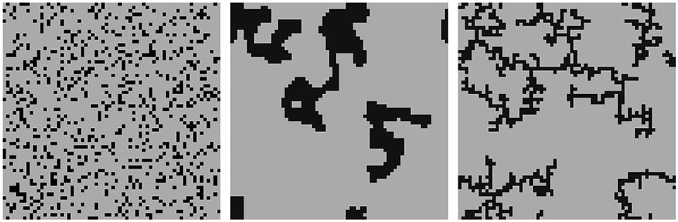
Figure 9. Effects of charges in solid restructuring: Initial configuration for both simulations, porosity θ = 0.8 (left), quasi stationary configuration without charges (middle), and quasi stationary configuration with randomly distributed charges dominating the restructuring (right).

3.4. Effect of Henry's Law and Gas Phase

In this section, we combine the restructuring of phases according to the CAM with the PDE model to illustrate the capability of our comprehensive model: A three phase system (as in Figure 6) is taken into account without any electric field or charges (33% solid, 33% fluid, 33% gas cells randomly distributed), cf. the picture on the left in Figure 10. Within the gas phase and the fluid phase a constant distribution of a species of 4 and 2 [1/L²], respectively, is present initially. It is degraded with a first order rate and rate constant −0.375 [1/T] in the fluid phase representing, e.g., the consumption of a nutrient, such as oxygen by aerobic organisms in the fluid phase. The diffusion is faster in the gas phase (D = 10⁻⁴ [L²/T]) compared to the fluid phase (D = 10⁻⁸ [L²/T]) and the transfer between the phases is determined via Henry's law with solubility constant $H_r^{\Gamma \mathrm{\text{LG}}}=2$. The picture on the right in Figure 10 shows the resulting distribution of the phases and species after the PDEs for the species are solved and the CAM is run simultaneously 50 steps on a domain of 64 × 64 cells. It is evident that the phase transfer determined by means of Henry's law, leads to a jump in the nutrient concentration across fluid–gas interface and therefore to a non-uniform distribution of the nutrient in the pore space. Moreover, concentration gradients are visible in the fluid and gas phases which become more prominent for lower diffusivity. This leads to nutrient-poor and nutrient-rich regions within the created aggregate structure.

FIGURE 10

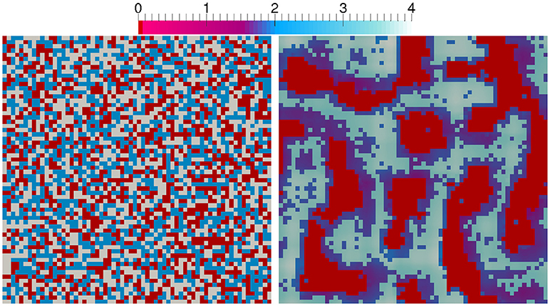
Figure 10. Aerobic bacteria in fluid phase combined with solid restructuring and gas reorganization: The scale depicts the concentration of a nutrient. Thus, solid cells are red, fluid cells are violet to dark blue, and gas cells are pale blue to white in the right picture.

3.5. Effect of the Electrostatic Field in the Solution

In this section, we combine the restructuring of phases according to the CAM with the PDE model for movement of potentially charged species in solution. Thus, we show the interplay of ions in solution that adsorb to charged particles, i.e., we combine the CAM for charged solids with the PDEs for a charged fluid phase. The sorption of ions to the surfaces defined by

${\partial }_t{\omega }_r^{\Gamma ,\pm }=k(g({\omega }_r^{\pm })-{\omega }_r^{\Gamma ,\pm })=1[1/\text{T]}·\left(\frac{0.3[\text{L}]{\omega }_r^{\pm }}{1+0.3[{\text{L}}^2]{\omega }_r^{\pm }}-{\omega }_r^{\Gamma ,\pm }\right)$

changes the attraction of particles and the resulting structures. The left picture in Figure 11 shows the initial state of a randomly distributed solid with randomly charged surfaces (charge numbers between −4 and +4) on a domain of size 32 × 32 with $D_r=10^{-8}\left[{\text{L}}^2\text{/T}\right]$, $C_r=10^{-3}\left[{\text{IT}}^2\text{/M}\right]$, and the other physical constants set to 1.

FIGURE 11

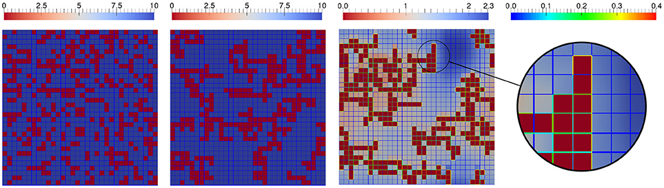
Figure 11. Interplay of ions in solution with charged solids: Initial configuration (first image) of solid (red), quasi stationary, final configuration of charged solid in neutral solution (second), and final configuration of charged solid in ionic solution (third image) when heterogeneous reactions alter the total charges of solid cells' edges. The zoom highlights charges on solid edges, the rainbow scale corresponds to the surface concentrations.

We compare the resulting structures under the influence of an uncharged chemical species and positively/negatively charged species. The uniform initial concentration of the uncharged species is 10 [1/L²] and homogeneous Neumann boundary is applied at the solid's surface Γ. Likewise, the uniform initial concentration of the positively charged chemical species is set to 10 [1/L²]. To ensure electroneutrality (also balancing the total charge of the solid), a negatively charged species with an initially homogeneous concentration of 13.27 [1/L²] is necessary (not plotted in Figure 11). The middle and right image in Figure 11 depict the quasi stationary, consolidated configurations of the solid (after 100 CAM steps with a stencil size of 3 [L]), when uncharged or charged species are considered, respectively. The inert uncharged species has remained constant at 10 [1/L²] as depicted in the middle picture of Figure 11. For the charged species heterogeneous reactions with the solid are included which alter the solid's charge and thus also the structure formation. In the zoom in the right of Figure 11 we see high surface concentrations of the charged species near high concentrations in the solute, and vice versa. The altered surface concentrations by sorption have an impact on the attraction of the solid particles and thus on the resulting solid structure, this becomes evident when comparing the aggregated particles in the respective final states.

4. Conclusion and Outlook

In this research, we presented a comprehensive mathematical model for structure formation. A novel discrete–continuum approach was taken, combining a model of partial differential equations for charged, reactive multicomponent transport with a cellular automaton method for the interactive self-organization of solid, bio, fluid and gas phases. A thorough illustration by means of numerical simulations was performed. This versatile approach has the potential to study the interplay of different aggregation mechanisms in silico. The systematic evaluation of a broad range of scenarios for microaggregate formation—also in comparison to batch experiments addressing aggregate formation—is subject of current work and a forthcoming article. It addresses, e.g., electrostatic shielding in realistic configurations, and studies structure formation at various concentrations and particle type relationships.

Although our results have already contributed towards enhancing our understanding of structure formation and self organization in soils, there are several aspects that may be added to the model.

First, more research is needed to investigate unsaturated fluid flow. This was for instance done for non-evolving angular pore networks representing soil aggregates in Ebrahimi and Or (2016). Here continuum model approaches were combined with an individual model for microbial community. The superposition of the results weighted with aggregate size distributions made it possible to access scales of practical interest. Traditional mathematical upscaling in unsaturated conditions has been performed in Daly and Roose (2018) to illuminate the parametrization of Richard's equation. Likewise it is desirable to predict the water retention curve in our setting. Moreover, the transport limited availability of nutrients and their role for habitat could be investigated in further research. Such model extensions seem to be quite promising for further investigations of soil's functionality in the future.

Furthermore other process mechanisms could be identified to broaden the applicability of our model. Those have to be determined and validated with the help of experimental studies which itself is a challenge. One step into that direction would be a model extension with respect to disaggregation of the resulting structures. Different aggregation and disaggregation mechanisms and their respective ratios need to be investigated. Moreover, building units and their composites (i.e., smaller units of building units) naturally undergo some random movement (representing self diffusion) independently of the CAM rules. Such a movement depending on the respective size of the particles needs to be included into the model. A related research question is how time scales are related to diffusion and how interaction processes can be balanced in a reasonable way.

Finally, a quantitative evaluation of the resulting structures would be possible by means of Minkowski functionals and further geometric measures characterizing among others the connectivity and compactness of a structure.

Author Contributions

AR discretized and implemented the numerical model, and conducted the simulations. KT contributed to developing the modeling concepts and process mechanisms. AP contributed to the model development, the design of the simulation studies and the interpretation of the results. NR developed the model concepts and formulations, and the simulation scenarios.

Conflict of Interest Statement

The authors declare that the research was conducted in the absence of any commercial or financial relationships that could be construed as a potential conflict of interest.

Acknowledgments

This research was kindly supported by the DFG RU 2179 “MAD Soil—Microaggregates: Formation and turnover of the structural building blocks of soils”. Discussion within the RU significantly promoted the present research. We particularly appreciate the input of Thomas Ritschel (Friedrich-Schiller Universität Jena) and Stefan Dultz (Leibniz Universität Hannover), and thank our students Andreas Meier and Markus Musch.

References

Aizinger, V., Rupp, A., Schütz, J., and Knabner, P. (2018). Analysis of a mixed discontinuous Galerkin method for instationary Darcy flow. Comput. Geosci. 22, 179–194. doi: 10.1007/s10596-017-9682-8

CrossRef Full Text | Google Scholar

Benioug, M., Golfier, F., Oltean, C., Buès, M., Bahar, T., and Cuny, J. (2017). An immersed boundary-lattice Boltzmann model for biofilm growth in porous media. Adv. Water Resour. 107, 65–82. doi: 10.1016/j.advwatres.2017.06.009

CrossRef Full Text | Google Scholar

Bennett, R., and Hulbert, M. (1986). Clay Microstructure. Dordrecht: Springer.

Google Scholar

Carminati, A., Benard, P., and Ahmed, M. (2017). Liquid bridges at the root-soil interface. Plant Soil 417, 1–15. doi: 10.1007/s11104-017-3227-8

CrossRef Full Text | Google Scholar

Crawford, J. W., Deacon, L., Grinev, D., Harris, J. A., Ritz, K., Singh, B. K., et al. (2012). Microbial diversity affects self-organization of the soil–microbe system with consequences for function. J. R. Soc. Interface 9, 1302–1310. doi: 10.1098/rsif.2011.0679

PubMed Abstract | CrossRef Full Text | Google Scholar

Daly, K. R., and Roose, T. (2018). Determination of macro-scale soil properties from pore-scale structures: model derivation. Proc. R. Soc. Lond. A Math. Phys. Eng. Sci. 474, 1–19. doi: 10.1098/rspa.2017.0141

PubMed Abstract | CrossRef Full Text | Google Scholar

Ebrahimi, A., and Or, D. (2016). Microbial community dynamics in soil aggregates shape biogeochemical gas fluxes from soil profiles–upscaling an aggregate biophysical model. Glob. Change Biol. 22, 3141–3156. doi: 10.1111/gcb.13345

PubMed Abstract | CrossRef Full Text | Google Scholar

Liang, Y., Hilal, N., Langston, P., and Starov, V. (2007). Interaction forces between colloidal particles in liquid: theory and experiment. Adv. Colloid Interface Sci. 134–135, 151–166. doi: 10.1016/j.cis.2007.04.003

PubMed Abstract | CrossRef Full Text | Google Scholar

Ray, N., Rupp, A., and Prechtel, A. (2017). Discrete-continuum multiscale model for transport, biomass development and solid restructuring in porous media. Adv. Water Resour. 107, 393–404. doi: 10.1016/j.advwatres.2017.04.001

CrossRef Full Text | Google Scholar

Rupp, A., and Knabner, P. (2017). Convergence order estimates of the local discontinuous Galerkin method for instationary Darcy flow. Numer. Methods Partial Differ. Equat. 33, 1374–1394. doi: 10.1002/num.22150

CrossRef Full Text | Google Scholar

Rupp, A., Knabner, P., and Dawson, C. (2018). A local discontinuous Galerkin scheme for Darcy flow with internal jumps. Comput. Geosci. 22, 1149–1159. doi: 10.1007/s10596-018-9743-7

CrossRef Full Text | Google Scholar

Six, J., Bossuyt, H., Degryze, S., and Denef, K. (2004). A history of research on the link between (micro)aggregates, soil biota, and soil organic matter dynamics. Soil Till. Res. 79, 7–31. doi: 10.1016/j.still.2004.03.008

CrossRef Full Text | Google Scholar

Six, J., Elliott, E., and Paustian, K. (2000). Soil macroaggregate turnover and microaggregate formation: a mechanism for C sequestration under no-tillage agriculture. Soil Biol. Biochem. 32, 2099–2103. doi: 10.1016/S0038-0717(00)00179-6

CrossRef Full Text | Google Scholar

Sparks, D. L. (1989). Kinetics of Soil Chemical Processes. San Diego, CA: Academic Press.

Google Scholar

Tang, Y., and Valocchi, A. J. (2013). An improved cellular automaton method to model multispecies biofilms. Water Res. 47, 5729–5742. doi: 10.1016/j.watres.2013.06.055

PubMed Abstract | CrossRef Full Text | Google Scholar

Tang, Y., Valocchi, A. J., Werth, C. J., and Liu, H. (2013). An improved pore-scale biofilm model and comparison with a microfluidic flow cell experiment. Water Resour. Res. 49, 8370–8382. doi: 10.1002/2013WR013843

CrossRef Full Text | Google Scholar

Tisdall, J. M., and Oades, J. M. (1982). Organic matter and water-stable aggregates in soils. Eur. J. Soil Sci. 33, 141–163.

Google Scholar

Totsche, K. U., Amelung, W., Gerzabek, M. H., Guggenberger, G., Klumpp, E., Knief, C., et al. (2018). Microaggregates in soils. J. Plant Nutr. Soil Sci. 181, 104–136. doi: 10.1002/jpln.201600451

CrossRef Full Text | Google Scholar

Wieners, C. (2005). Distributed point objects. A new concept for parallel finite elements in Domain Decomposition Methods in Science and Engineering, Vol. 40 of Lecture Notes in Computational Science and Engineering, eds T. Barth, M. Griebel, D. Keyes, R. Nieminen, D. Roose, and T. Schlick (Berlin; Heidelberg: Springer), 175–182.

Google Scholar