The Potential of the Geostationary Carbon Cycle Observatory (GeoCarb) to Provide Multi-scale Constraints on the Carbon Cycle in the Americas

Introduction

Global trends in the atmospheric concentrations of carbon dioxide (CO₂) and methane (CH₄) are well established. The basic causalities for the observed trends are known; however, the spatial and temporal pattern of these perturbations and the flux dependence on the underlying processes are not well known (Stocker et al., 2013). The fundamental roadblock to advancing knowledge of the carbon cycle is uncertainty about land-atmosphere CO₂ and CH₄ fluxes (e.g., Cox et al., 2000; Friedlingstein, 2014).

Already, observations from space hold great promise. The Greenhouse Gas Observing Satellite (GOSAT) was launched in 2009 and is approaching a nearly continuous 10-year data record. With a relatively coarse spatial footprint (100 km²) and three-day revisit cycle, GOSAT was designed to make measurements that would constrain the carbon cycle at large scales in regions that are unobservable in the surface network, such as the tropical oceans. Numerous papers have assessed the ability of GOSAT to constrain surface emissions (e.g., Maksyutov et al., 2013; Houweling et al., 2015; Kondo et al., 2015; Wang et al., 2018), and the community looks forward to the launch of GOSAT-2.

The Orbiting Carbon Observatory-2 (OCO-2) is a 3-channel spectrometer, which measures the concentration of atmospheric carbon dioxide. It was successfully launched in 2014 to provide regular global coverage at high spatial resolution to better sample atmospheric CO₂ with the objective, like GOSAT, of providing a top-down constraint on surface fluxes. The coverage and density of measurements from OCO-2 is revealing patterns in atmospheric CO₂, which again were unobservable with the pre-existing ground-based network. The scientific community is developing strategies for generating estimates of CO₂ surface exchange from these measurements, and the spatial and temporal scales of GOSAT and OCO-2 observations mean that they will inform best exchanges at continental scales. Initial resulting are very promising (e.g., Eldering et al., 2017).

The need for observations at finer spatiotemporal scales (e.g., Sellers et al., 2015) led, in part, to NASA's recent selection of the Geostationary Carbon Cycle Observatory (GeoCarb) as the Earth Venture Mission-2 (EVM-2). GeoCarb is a 4-channel, slit-scan spectrometer that will measure absorption spectra at wavelengths 1.61, 2.06, and 2.32 μm in sunlight reflected from the land to retrieve total atmosphere-column amounts of CO₂, CH₄, and carbon monoxide (CO) from GEOstationary orbit (GEO). As with OCO-2, oxygen measurement at 0.76 μm enables the retrieval of column integrated concentrations of CO₂, CH₄, and CO (i.e., dry-air mixing ratios X_CO2, X_CH4, and X_CO), from which the community will infer terrestrial fluxes of CO₂ and CH₄, and attribute them to either biogenic or anthropogenic processes utilizing CO and other information. The slit-scan concept, described below, will allow GeoCarb to deliver concentrations at least daily at fine (10 km) spatial scales over the Americas for terrestrial flux calculations to directly test and extend our understanding of biogeochemical processes.

The chosen spectral channel (0.76 μm) for total column oxygen includes Fraunhofer lines from which Solar-Induced Fluorescence (SIF) can be retrieved (e.g., Frankenberg et al., 2014). SIF is quasi-proportional to plant photosynthetic activity, though the constant of proportionality is dependent on many factors that are being quantified with field studies, including vegetation type and spatiotemporal scales of interest (e.g., Damm et al., 2012; Guanter et al., 2014).

In this paper, we provide an outline of the GeoCarb mission and some simulation studies that indicate the potential for a transformative set of measurements, as well as pointing to some of the issues to be resolved before GeoCarb launches in 2022.

Background

Scientific Challenge

Emission quantification for urban and industrial areas was one of the reasons to use a geostationary orbit and an instrument with the capability to make daily wall-to-wall measurements (Sellers et al., 2015) over terrestrial regions at fine spatial scales. The GeoCarb observations directly address urban emissions, which are the most rapidly growing source of CO₂ (Stocker et al., 2013) and an increasingly important source for CH₄ (Stocker et al., 2013).

GeoCarb's persistent fine-scale daily mapping measurements under changing conditions should enable significant advances on an important range of challenging CO₂ biotic issues, including: CO₂ fertilization (e.g., Schimel et al., 2015), change in primary production because of nitrogen deposition (e.g., de Viesa et al., 2009), and the influence of broad climatic patterns (e.g., El Niño and La Niña) on terrestrial sources and sinks (Houghton, 2000; Sellers et al., 2018). This probes the mechanisms of the observed inter-annual variability in the atmospheric concentration of CO₂ (e.g., Figure 4 of Le Quéré, 2018), and it is the pattern of this variability that sets the mission timeframe of 3 years (Rayner et al., 2008). The GeoCarb mission attacks the primary question of the nature of the net terrestrial sink of CO₂.

Wetland ecosystems, rice paddies and livestock are major, and highly uncertain, sources of CH₄ (Kirschke et al., 2013). Several approaches have been used to scale up from measurements at individual plots to estimations of CH₄ emissions at the landscape scale. However, there has been little large-scale top-down validation. Industrial sources are also poorly quantified (Miller et al., 2013). The IPCC states that there are “large uncertainties in the current bottom-up estimates of components of the global source [of methane], and the balance between sources and sinks is not yet well known” (Stocker et al., 2013)^.The GeoCarb's high space- and time-measurements of CH₄ enable important analyses of human impacts via agriculture and industry vs. natural phenomena on methane sources.

The GeoCarb measurements of CO concentrations and SIF provide essential information for CO₂ and CH₄ source attribution. For example, CO helps distinguish between biotic fluxes of CO₂ and CH₄ from fluxes associated with combustion (Palmer et al., 2006; Rayner et al., 2014). SIF measurements are directly related to gross primary production (GPP; photosynthesis), and when coupled with inversions of concentrations, SIF can support partitioning of Net Ecosystem Exchange (NEE) into GPP and ecosystem respiration. Determination of GPP, NEE, and ecosystem respiration will increase our capability to elucidate fundamentally key elements of the Carbon-Climate connection (Sellers et al., 2015).

Instrument Design and Trace Gas Retrievals

The GeoCarb instrument will be hosted on a SES Government Solutions (http://www.ses-gs.com) satellite in GEO orbit at 85° (±15°) West longitude, and it will be launch in 2022. The ~85°W slot allows observations of major urban and industrial regions, large agricultural areas, and the expansive South American tropical forests and wetlands, which will help resolve climate-critical flux variability for CO₂ and CH₄ (Sellers et al., 2015). GeoCarb deploys, as noted, a 4-channel slit imaging spectrometer that measures reflected near-IR sunlight at wavelengths 1.61 and 2.06 μm for column integrated CO₂ dry air mixing ratio (X_CO2), and 2.32 μm for X_CH4 and X_CO. The fourth channel, 0.76 μm, measures total column O₂, which allows determination of mixing ratios. The 0.76 μm channel also allows measurement of SIF and provides valuable information on aerosol and cloud contamination (Taylor et al., 2012; Nelson, 2015). It is worth noting that the O₂ and CO₂ channels are similar to those used for the OCO-2 mission and that the O₂ spectral band is identical to that of OCO-2.

The retrieval of SIF, X_CO2, X_CH4, and X_CO is accomplished through the use of an optimal estimation technique that draws upon the heritage of the Atmospheric Carbon Observing System (ACOS) algorithm developed initially for OCO and GOSAT, and with numerous refinements updates for OCO-2 (e.g., O'Dell et al., 2012, 2018; Wunch et al., 2017). In brief, a first guess of each gas profile as well as other atmospheric parameters are propagated through a radiative transfer model to produce a simulated spectra, which is compared against the measured spectra in each band. The difference between the simulated and measured spectra is propagated back into updated gas concentrations and atmospheric parameters, and the process is repeated until the algorithm converges. SIF is produced separately by a different algorithm, called the Iterative Maximum a Posteriori Differential Optical Absorption Spectroscopy (IMAP-DOAS, Frankenberg et al., 2005) algorithm, which is also used to screen clouds. GeoCarb will employ the OCO-2 algorithm, modified to include the longest wavelength band, in which OCO-2 does not take spectra.

The instrument scan slit design allows for a large North-South (N-S) extent with high spatial resolution along the scan. The on-board N-S extent of the scan is fixed at a 4.4° view angle, which corresponds to 25° in latitude or 2,800 km at nadir on the Earth's surface. Each scan is composed of 1016 N-S samples spaced 2.7 km apart on center and collected with 3 km East-West (E-W) double sampling. Scans involve a 4.08-s integration time, followed by a 0.3825s E-W step. This instrument configuration allows GeoCarb to scan the conterminous United States (CONUS) in <2.5 h. The scan patterns are flexible; scan blocks can be changed, and the scan strategy can be updated to observe areas of greater interest or uncertainty, for calibration and validation, or for transient events in a campaign mode. Figure 1 shows a sample coverage map for the Mexico City area for both OCO-2 and GeoCarb. By sweeping the slit from East to West, GeoCarb provides continental-scale “mapping-like” coverage, producing daily maps of X_CO2, X_CH4, X_CO, and SIF over regions of interest, which enables CO₂ and CH₄ flux estimation and attribution at unprecedented temporal and spatial scales.

FIGURE 1

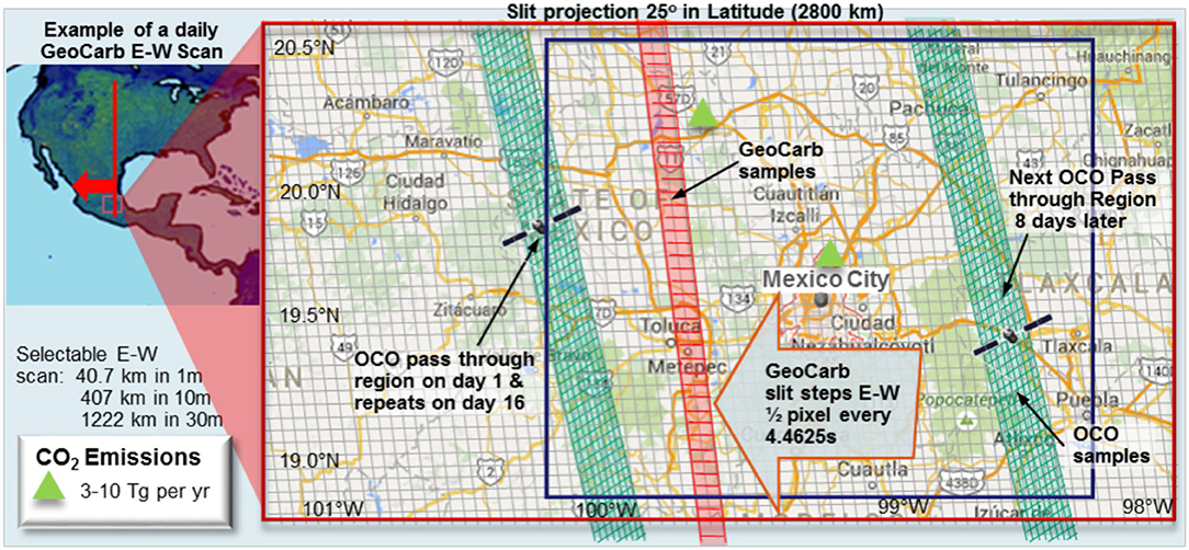
Figure 1. Sample field of view for the area surrounding Mexico City. The green parallelograms represent individual OCO-2 soundings, and each track is traversed in a few minutes, but with a 16 day latency between revisits. By comparison, the red rectangles represent individual GeoCarb soundings, and the shaded region depicts a single observing slit projection. Every 4.4625s, the shaded red area will shift a half width to the left, allowing the area to be scanned in full in a few minutes. The map of North America in the upper left shows the full N/S extent of the slit projection. The green triangles represent power plants that produce 3–10 TgC per year in emissions. GeoCarb would make it possible to verify the reported emissions rates with top down emissions estimates.

Science Hypotheses

The ~85°W slot enables, as mentioned, observations of most major urban and industrial regions in the Americas, large agricultural areas, and the expansive South American tropical forests and wetlands. Each of these regions plays a key role in the global carbon cycle, and thus GeoCarb observations will help to provide a climate-critical insight into the Carbon-Climate connection (Cox et al., 2000; Friedlingstein, 2014; Sellers et al., 2018) as well as monitoring large “point” sources (e.g., cities) of all three gases, and helping to disaggregate anthropogenic and biogenic emissions using all three gases in tandem.

Several Observing Systems Simulation Experiments (OSSEs) were performed in order (a) to determine useful measurement requirements that are technically feasible and (b) to examine the potential for significant scientific advances that will be made possible with observations from GeoCarb. These OSSEs were designed with a set of hypotheses in mind, though there are numerous other important questions that could be addressed.

Hypothesis 1: The ratio of the CO₂ fossil source to biotic sink for the conterminous United States (CONUS) is ~4:1. Top down flux estimates constrained by the surface network have large posterior uncertainties relative to the magnitude of the fluxes themselves. For example, the 2000–2014 mean biological sink as estimated from CarbonTracker [Peters and Jacobson (2007) with regular updates at https://www.esrl.noaa.gov/gmd/ccgg/carbontracker/] for temperate North America is about 0.4 PgC/year, but the reported uncertainty in this estimate is ~0.75 PgC/year. The Modeling Atmospheric Composition and Climate (MACC) re-analysis product (http://macc.copernicus-atmosphere.eu/about/documentation/global/; Chevallier et al., 2010) estimates the sink for the sample year of 2005 to be 0.6 PgC/year stronger than that of CarbonTracker for the same year (i.e., 0.8 and 0.2 PgC/year, respectively). Complicating this issue is the presence of large fossil sources concentrated in the extratropical Northern Hemisphere. The annual total fossil source is about 1.5 PgC/year for the US, with 7% uncertainty on the total. The mean net sink is about 0.4 PgC/year (according to CarbonTracker), with an uncertainty of ~1 PgC/year. By using a regional scale OSSE over the conterminous United States (CONUS), we demonstrate that in the presence of correlated random observation errors (see section Observing System Simulation Experiments for details) over moderate length scales (200 km), observations from GeoCarb will still be sufficient to constrain anthropogenic and biogenic emissions at the regional scale.

Hypothesis 2: Variation in productivity controls the spatial pattern of terrestrial uptake of CO₂. Previous work shows large differences in global Gross Primary Production (GPP) estimates from ecosystem models. For example, Table 3 of Yan et al. (2014) find a range of larger that 50 PgC/year from small collection of models. A more diverse ensemble from the most recent Climate Model Intercomparison Project (CMIP5) finds even larger differences (Kathe Todd-Brown, personal communication). For example, the BCC-CSM 1.1 model predicts 131 PgC/year while the IPSL-CM5A model predicts 218 PgC/year, which is an 87 PgC/year difference. This indicates a large uncertainty in the amount of carbon being taken up annually by the terrestrial biosphere.

Numerous papers in the literature (e.g., Guanter et al., 2014) have demonstrated the strong linear relationship between SIF and GPP, and specifically on determining parameterizations of the SIF-GPP coupling for different ecosystems and species. Frankenberg et al. (2011) demonstrate that SIF from GOSAT is strongly correlated with monthly GPP at larger scales of a few hundred kilometers. Additionally, recent work demonstrates the ability to estimate monthly GPP using the photosynthesis model SCOPE together with SIF retrieved from OCO-2, with a global uncertainty of ~2% (Norton et al., 2018).

Coupling SIF-derived estimates of GPP with satellite inversions of X_CO2 to infer net terrestrial carbon storage allows the separation of NEE into its component parts: GPP and ecosystem respiration (R_eco), including fire. Being able to isolate R_eco, including the separation of the fire component via CO measurements and thereby isolate biotic respiration, 0.76 μm, will be extremely valuable in probing the carbon-climate system. For instance, GeoCarb SIF retrievals and fluxes derived from X_CO2 will be used to test the hypothesis that GPP is much more sensitive to disturbance than respiration.

Hypothesis 3: The Amazonian Forest is a significant (0.5–1.0 PgC/year) net terrestrial sink for CO₂. The Amazon is a key player in the global carbon sink, as well as one of the most fragile in terms of carbon-climate sensitivity. The lack of measurements in the tropics, however, make quantitative statements about the uptake in the Amazon basin difficult. Even OCO-2 struggles to make observations over this perennially cloudy region, though recent progress with cloud screening algorithms will likely improve coverage. GeoCarb, in concert with geostationary meteorological observatories such as ABI on GOES-16/17, has the potential to scan regions that are clear at different times of day and different seasons in the year. To test the capabilities of GeoCarb to capture anomalies in productivity and its associated flux, several experiments were performed in which estimates from CASA-GFED (Carnegie-Ames-Stanford-Approach biogeochemical model with the Global Fire Emissions Database) were inflated by different percentages to explore the uncertainty space related to this question.

Hypothesis 4: Tropical Amazonian ecosystems are a large (50–100 PgC/year) source for CH₄. The cycle of CH₄ in the tropics is the subject of much debate in the literature and is strongly tied to temperature and precipitation. The cycle is also affected by inundation and the resultant microbial activity, which are difficult to measure. Bloom et al. (2016) conducted simulation experiments to address satellite constraints on biogeochemical processes and concluded that a geostationary satellite is necessary to observe with sufficient frequency to constrain regional CH₄ emissions in tropical South America. As an example, regional emissions from MACC II (e.g., Massart et al., 2014) for 2011 and 2012 were dramatically different. In the surface flask constrained MACC CH4 emissions, the 2012-2011 August emissions difference was positive north of the Amazon river and negative south of the Amazon river, i.e., the data-informed efflux was stronger north of the Amazon in 2012 than 2011, and vice versa south of the Amazon river.

Hypothesis 5: The CONUS methane emissions are a factor 1.6 ± 0.3 larger than in the EPA database. There are numerous estimates of CH₄ emissions in the US, the majority of which are greater than those of the United States Environmental Protection Agency (EPA). For example, Miller et al. (2013) produced top-down CH₄ estimates using aircraft that are ~1.5 times the EPA values for the total, and much greater for certain industries (e.g., livestock emissions are twice as much as some inventories) and in certain regions (the South-Central totals were ~2.7 times larger than inventories). Recent results show that the topic remains in flux (e.g., Alvarez et al., 2018). Even more, there are large discrepancies in estimates of “fugitive” emissions from fossil fuel production, which amount to leakage at different stages of the production process. Numerous studies (e.g., Brandt et al., 2016) conclude that the vast majority of fugitive emissions are from a small number of large “super-emitters.” Locating large point sources draws interest from both the environmental monitoring community and the fossil fuel industry, for whom fugitive CH₄ emissions represent lost revenue.

Hypothesis 6: Larger cities are more CO₂ emissions efficient than smaller ones. Multiple hypotheses exist for the manner in which emissions from urban areas scale with population. For example, Fragkias et al. (2013) proposes a linear relationship, while Bettencourt (2013) suggests a scaling law of 1.15. Using the idealized framework in Rayner et al. (2014), the uncertainty on monthly, 25 km² emissions is computed in the presence of targeted GeoCarb observations of CO₂ and CO that account for pollution and cloudiness typical of urban regions around the globe. CO serves as an important discriminant of anthropogenic emissions, in particular combustion, and so is critical for differentiating urban emissions. The uncertainty on the slope of emissions vs. size is estimated to be 12%, which is small enough to discriminate between the two hypotheses. This insight will aid in the process of urban planning, which is crucial for adaptation strategies needed to avoid the worst effects of climate change. Numerical experiments with Shanghai as the target indicate that the idealizations related to clouds, aerosols and the spatial distributions of sources in the work of Rayner et al. do not influence these conclusions significantly (O'Brien et al., 2016).

Observing System Simulation Experiments

To establish measurement requirements on mixing ratios needed to meet targeted flux estimates, the GeoCarb team performed numerous Observing System Simulation Experiments (OSSEs) under various assumptions of mixing ratio measurement accuracy. To encompass the range of science issues, we used different techniques for these OSSEs, including concentration signal detection experiments, posterior flux uncertainty reduction calculations, and atmospheric inversions with biased and unbiased priors.

The OSSEs described below were performed at both regional scales (~100 km) and local scales (~10 km). The sounding location selection was treated differently for each experiment. Previous work by Polonsky et al. (2014) assessed the feasibility of detecting plumes under the assumption of different wind speeds with different numbers of samples, and the experiments in O'Brien et al. (2016), on which the results for Hypothesis 6 are based, follow the same procedure by assessing the impacts with different numbers of soundings for an urban region. At regional scales, the flexibility of scanning, as well as the limitation due to number of hours of solar illumination per day, introduce the potential for an optimization of scanning to meet different science goals. In this work, we utilize the simplest scanning scheme possible where all spatial regions are scanned once per day, and this is described in section Scanning Strategy. The pseudo-data used in each case utilized a single sounding uncertainty, described in section Single Sounding Uncertainty For the regional OSSEs, the single soundings were aggregated to ~100 km scale for computational purposes, and the treatment of the uncertainties in this aggregation are described in section Aggregated Observational Uncertainty. A brief discussion of community requirements for SIF is presented in section Solar Induced Fluorescence Measurement Requirements. The models used in the regional scale and local scale OSSEs are described in sections Regional/Continental Scale Modeling Framework and Urban Scale Modeling Framework, respectively.

Scanning Strategy

For the urban scale OSSEs, scanning frequency was treated as a quantity of interest. Results are reported in Polonsky et al. (2014), Rayner et al. (2014), and O'Brien et al. (2016). For the regional scale OSSEs, as mentioned above, the scanning strategy selected is also a potential optimization problem. For the OSSEs performed in this study, a simple strategy, described in the next paragraph, was chosen with optimization of the scanning left for future work.

The land mass between 50°S and 50°N was divided into four scan blocks as shown in Figure 2. The blocks were scanned in the same order every day, with the starting time for the scanning selected empirically to maximize the number of soundings by month according to seasonal variations of sunlight. The scanning order is: Tropical South America, Subtropical South America, Temperate North America, Tropical North America, Tropical South America, Temperate North America. Depending on season, this allows for up to two revisits to the Amazon and the conterminous United States (CONUS per day), allowing the experiments to target the science questions above effectively. The observing sequence assumes 4.46s per 1016 footprints N/S, and the total time for each scan block is just 4.46s times the number of slits necessary to cover the land mass in the scan block.

FIGURE 2

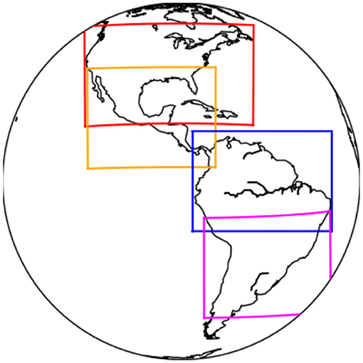
Figure 2. Scan blocks used in regional OSSE experiments. The blocks are named for the region they primarily cover: Temperate North America (red), Tropical North America (orange), Tropical South America (blue), and Subtropical South America (magenta).

Single Sounding Uncertainty

O'Brien et al. (2016) presented an OSSE that is motivated by introducing more realism into the earlier study by Rayner et al. (2014). The assumption of a constant 10% cloud free scenes in Rayner et al. (2014) was thought to be optimistic for urban regions, as the diurnal cycle of cloud and aerosol in urban environments is complex. Additionally, Rayner et al. (2014) assume a static uncertainty for all clear scenes, where “clear” means that the Cloud-Aerosol Lidar and Infrared Pathfinder Satellite Observation (CALIPSO) observed a scene with OD < 0.3. With these considerations in mind, O'Brien et al. (2016) designed an end-to-end experiment in which realistic atmospheric fields were simulated using the Weather Research and Forecasting model along with the chemistry component (WRF-Chem). The fields included the typical atmospheric state variables as well as numerous tracers, including CO₂, CH₄, CO, cloud water and ice, and various aerosol species. These fields were used to simulate spectra, which were then presented to a retrieval algorithm similar to those used by OCO-2 and GOSAT [ACOS, O'Dell et al. (2012)], to produce retrieved X_CO2, X_CH4, X_CO, and other parameters. Model error arose for the retrieval's ability to adjust a limited parameter set, such as the aerosol optical depth and type, but not other key optical properties of those aerosols, which were treated in a more sophisticated way within WRF-Chem.

The retrieval algorithm produces not only column concentrations, but also an estimate of the uncertainty in those concentrations. With the complete knowledge of the atmospheric state, the signal to noise ratio (SNR) can be calculated. The relationship between SNR and posterior uncertainty was parameterized with a function of the form $\sigma =\frac{a}{(1+bSN{R}^c)}$ for each species. The coefficients a, b and c are given in Table 8 of O'Brien et al. (2016), and are reprinted here in Table 1. These functional relationships are used to estimate single sounding uncertainties in all the OSSEs.

TABLE 1

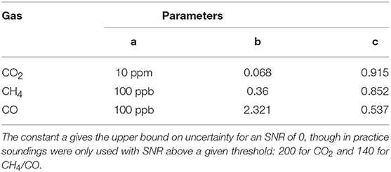
Table 1. Constants for uncertainty parameterization as a function of SNR as in O'Brien et al. (2016).

To compute uncertainty, we first compute $SNR=\frac{I}{N}$. The signal value I is given by the relationship:

$\begin{array}{cc}\begin{array}{r}I={\alpha }_E\frac{F_{sun}}{\pi }\end{array}& (1)\end{array}$

where $\frac{F_{sun}}{\pi }$ is the top of atmosphere solar irradiance, and α_E is the “effective albedo” that incorporates surface reflectance and attenuation by scatterers:

$\begin{array}{cc}\begin{array}{r}{\alpha }_E=\alpha cos(SZA)exp(-m\tau )\end{array}& (2)\end{array}$

Here α is the MODIS MCD43C3 white sky albedo (Band 6 for CO₂ and Band 7 for CH₄/CO), m is the airmass factor (i.e., $m=\frac{1}{cos(SZA)}+\frac{1}{cos(ZA)}$ for the solar zenith angle SZA and sensor zenith angle ZA), and τ is the OD of clouds and aerosols, taken from 5° × 5° monthly histograms of CALIPSO total OD (e.g., as was used in Crowell et al., 2018). The noise is derived from the instrument model:

$\begin{array}{cc}\text{N}=\sqrt{{\text{N}}_{\text{0}}^{\text{2}}{\text{+N}}_{\text{1}}\text{I}}& (3)\end{array}$

with band-specific empirical parameters that relate instrument design to a signal independent noise term N₀ and signal dependent noise term N₁, given in Table 2.

TABLE 2

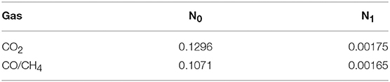
Table 2. Noise model coefficients used to calculate SNR and the resultant uncertainties for each retrieved gas.

Single sounding uncertainty curves for each gas are given by Figure 11 of O'Brien et al. (2016). All uncertainties decrease as SNR increases, with X_CO2 bounded above by ~1.0 ppm for SNR >200, X_CH4 bounded above by ~5 ppb and X_CO by ~3 ppb for SNR >150. Also included in this plot are “actual errors” that show the result of the inadequacies of the forward model. These actual errors are used in the urban scale uncertainty reduction calculations. In the regional scale OSSEs, this additional error is assumed to be part of an irreducible error component that is described in the next section.

Aggregated Observational Uncertainty

In the regional OSSEs, the individual GeoCarb footprints are not used. Rather, in the spirit of Baker et al. (2010) and Crowell et al. (2018), an effective “super-observation” of soundings is calculated at the resolution of the inversion model. To use this approach, we must estimate the uncertainty at the scale of the model, which is ~100 km. This is modeled using an uncorrelated random error component and a correlated/systematic error component. We assume that the random error component, computed as detailed in section Single Sounding Uncertainty, reduces by the square root of the number of soundings. The correlated/systematic error component is treated as irreducible, in line with the conclusions of (Kulawik et al., 2016).

The systematic error component for GeoCarb cannot be known in advance, so we must make a reasonable estimate. These errors will tend to be worse for high view and solar zenith angles due to lower signals and larger cloud and aerosol effects. We parameterize the single-sounding systematic error term for CO₂ as a function of air mass factor m: σ_sys(m) = 0.3 ppm + 0.2 ppm × (m-2), where the constant is based on Kulawik et al. (2016) and derived from comparisons GOSAT/OCO-2 and the Total Column Carbon Observing Network (TCCON). For methane, we set σ_sys(m) = 6 ppb + 2 ppb × (m-2); O'Brien et al. (2016) indicates that the constant term in σ_sys could be as low as 3 ppb.

For sampling, we compute the SNR and exclude any soundings with SNR <200 for CO₂ and SNR <150 for CH₄ and CO. We also exclude soundings in which the two-way slant optical depth τ(in)/cos(SZA) + τ(out)/cos(ZA) is >0.6. The mean value of X_CO2 at 1° × 1° then has a total uncertainty ${\sigma }_{XCO2}=\sqrt{{{\sigma }_{sys}}^2+\frac{{{\sigma }_p}^2}{n}}$, where n is the number of soundings that have sufficient SNR and meet the OD threshold. In this way, σ_XCO2 varies from ~0.3 ppm at low view and zenith angles and multiple high SNR soundings to about 3 ppm for a large airmass factor and a minimal number of low SNR soundings. To account for correlations between systematic errors of neighboring 1° × 1° mean values, we further inflate the 1° × 1° errors by a factor of 2.5, which assumes a spatial de-correlation length of 2° for the correlated/systematic error. The 1° × 1° errors for June 1 and December 1 (without the extra scaling by 2.5) are shown in Figure 3. As might be expected, the aggregated uncertainties are largely dominated by the systematic component at regional scales, due to the large number of soundings in each 1° × 1° grid box.

FIGURE 3

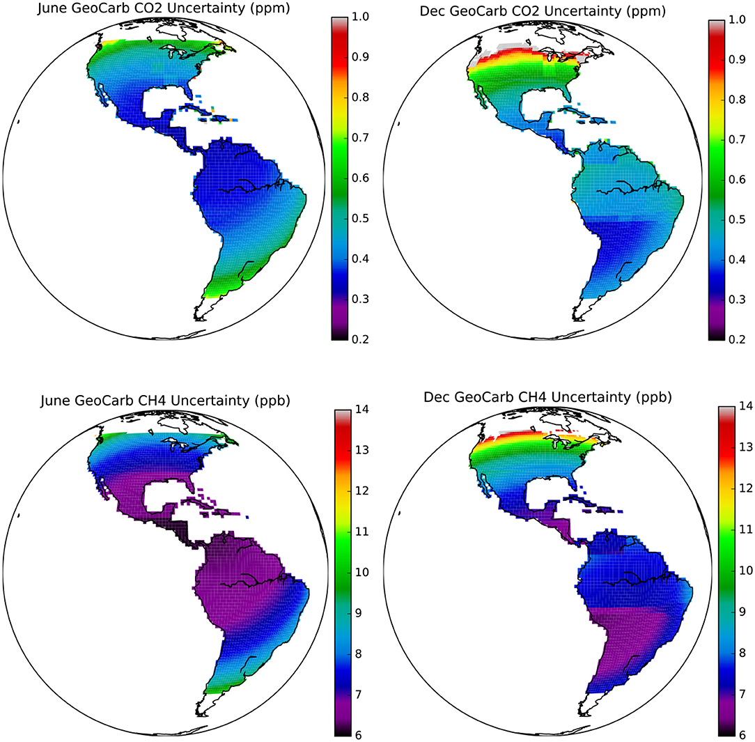
Figure 3. GeoCarb 1° × 1°CO₂ uncertainty (Top) and CH4 uncertainty (Bottom) consisting of both random and correlated systematic errors, but without the extra scaling by 2.5 that accounts for a spatial correlation length scale of 2°. For June (Left), the uncertainties are largely driven by the systematic errors parametrized in terms airmass factor, while in December (Right), we see the impacts of cloudiness and lower surface albedos in the Amazon region in the reduced number of soundings as evinced by the larger uncertainties than would be apparent in airmass alone.

Crowell et al. (2018) found that for narrow swath polar orbiting satellites such as OCO-2, transport errors were on the order of 0.5 ppm. No transport errors are explicitly included in the regional simulations, as they are expected to be small given the daily revisit cycle of GeoCarb. The impact of transport errors on flux inversions is a long-standing topic of interest in the atmospheric community, and the assertion of reduced transport errors will be tested in future work.

Solar Induced Fluorescence Measurement Requirements

Diurnal SIF data from laboratory and field observations suggest a SIF measurement requirement for diagnosing variability in GPP and plant physiology changes due to stress is 13–20% of peak SIF (~2–2.5 W m⁻² nm⁻¹ sr⁻¹). GeoCarb will have sufficient spectral resolution (equivalent to that of OCO-2) to meet this requirement.

Regional/Continental Scale Modeling Framework

The experiments performed for Hypotheses 1, 2, 3, and 4 in section Background utilize the atmospheric tracer transport model TM5 (Krol et al., 2005). TM5 translates surface emissions into atmospheric concentrations using the ERA-Interim (Dee et al., 2011) meteorological fields at 1° by 1°. To produce pseudo-observations, the resultant model concentrations are sampled with a pressure weighted averaging kernel to produce column concentrations of X_CO2 and X_CH4. Uncertainties are assigned as discussed in 3.2 and 3.3 at 1° by 1° resolution. For the flux inversion experiments that address Hypotheses 1 and 2, the Four Dimensional Variational (4DVAR) data assimilation algorithm is used (e.g., Basu et al., 2013; Babenhauserheide et al., 2015; Crowell et al., 2018) to estimate surface fluxes that best match the observed concentrations.

Urban Scale Modeling Framework

Hypothesis 5 is addressed using the framework discussed in Rayner et al. (2014). Briefly, a Gaussian plume model is driven by WRF derived winds that are appropriate for different regions (e.g., Shanghai and Mexico City) to generate concentrations that are sampled to create pseudo-data, which is perturbed as in Rayner et al. (2014). The uncertainty reduction is computed using the method of Rayner and O'Brien (2001).

Results and Discussion

The results are broken down by Hypothesis. Where necessary, further details specific to each experiment (e.g., prior uncertainties) are elucidated for clarity.

Hypothesis 1: The Ratio of the CO₂ Fossil Source to Biotic Sink for CONUS Is ~4:1

TM5-4DVAR was employed to compute the expected uncertainty reduction in surface fluxes for this hypothesis. In this OSSE, the ensemble of prior fluxes is composed of statistical perturbations of truth fluxes that is built from the Carnegie-Ames-Stanford Approach (CASA, Potter et al., 1993) biogenic fluxes and the Global Fire Emissions Database Version 3 for fire fluxes (GFEDv3, Takahashi et al., 2009; van der Werf et al., 2010) for ocean fluxes, and fossil fuel emissions from the Carbon Dioxide Information Analysis Center (CDIAC, Andres et al., 2015). The perturbations are random draws from a Gaussian distribution with mean zero and variance equal to the absolute value of the difference between the Lund-Potsdam-Jena (Sitch et al., 2003) and CASA land fluxes and the NCAR Ocean Biogeochemistry Model (Doney et al., 2009) and Takahashi fluxes for the ocean. No spatial or temporal correlations are included in the prior uncertainty.

A measure of information content of observations is how much the pseudo-data reduce the spread of the distribution, in this case measured by the Root Mean Square Error (RMSE) of the 50-member ensemble. The daily flux uncertainty reduction for a 1° × 1° regional inversion over CONUS is shown in Figure 4. The left panel shows the prior daily flux uncertainty (i.e., RMSE of the prior flux ensemble) for June; the right panel shows the reduction in RMSE (as a percentage of the prior RMSE) using a Monte Carlo ensemble of TM5-4DVAR flux inversions with 1° × 1° GeoCarb observations and errors as described above. In the most uncertain areas, GeoCarb achieves reductions of +75%, and 30–50% over much of the CONUS domain at the 1° × 1° pixel scale in for daily fluxes using 1 month of observations. Results improve significantly with longer observing times.

FIGURE 4

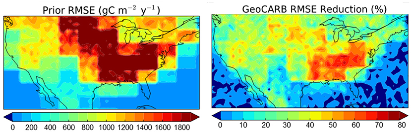
Figure 4. (Left) Prior uncertainty for the CONUS experiment for the month of June (expressed in gC m⁻² y⁻¹), equal to the absolute difference between the Lund-Potsdam-Jena [LPJ, (Sitch et al., 2003)] and CASA-GFEDv3 terrestrial fluxes. The majority of the prior uncertainty is in the growing regions of the US. (Right) The reduction in ensemble daily flux RMSE for June, expressed as a percentage, when GeoCarb pseudo-observations are used to update the perturbed prior fluxes.

The annual total fossil source is about 1.5 PgC/year for the US, with 7% uncertainty on the total. The mean net sink is about 0.4 PgC/year (according to CarbonTracker), with an uncertainty of ~1 PgC/year. The stated uncertainty reduction implies an aggregate net sink uncertainty of 0.15 PgC/year, on par with the fossil uncertainty, which supports the disaggregation of these two terms for the total US carbon budget.

Hypothesis 2: Variation in Productivity Controls on the Spatial Pattern of Terrestrial Uptake of Co₂

As noted earlier (Hypothesis Two), annual GPP estimates of North America from various models show large inter-model differences, ranging from 12 to 33 PgC per year. Such large uncertainty in model performance clearly indicates the limits of in-situ data (e.g., eddy flux tower sites) for model evaluation and calls for broader coverage from space-borne observations to evaluate models at regional to global scales. Laboratory and in situ observations show strong correlation between GPP and SIF; moreover, analysis of existing space-based oxygen A-band measurements has revealed that SIF can be usefully retrieved for about 80% of soundings.

The LEO missions make SIF observations at varying spatial resolutions [~30 km² for GOSAT and GOME-2; ~10 km² for OCO-2; ~0.1 km² for the Fluorescence Explorer (FLEX) mission] and temporal resolutions (16-days for OCO-2, nearly a month for GOME-2, GOSAT, FLEX). GeoCarb will make daily SIF observations at 5–10 km spatial resolution. In comparison to the current and future LEO missions (OCO-2, GOME-2, FLEX), GeoCarb SIF has more frequent revisits, similar spatial resolution and comparable radiometric precision. LEO missions generate gridded data products by using samples within a grid-cell (0.25°-1.0°) over 16 days to 30 days. The global land cover maps show landscapes within such a grid cell are diverse and have varying temporal dynamics. The footprint of GeoCarb is larger than OCO-2 and FLEX; however, since SIF measurements from GeoCarb are spatially additive, area averages will act as direct proxies for area-integrated SIF; no upscaling or multi-orbit averaging of spatial samples is required for gridded SIF products due to GeoCarb's mapping capability.

SIF reveals signals directly associated with photosynthesis; therefore, sub-daily measurements of SIF coupled with retrievals of net fluxes from X_CO2 across large environmental gradients provides a path to attributing terrestrial net CO₂ flux to variations in photosynthesis or respiration. The net fluxes (NEE) from inversion of mixing ratios combined with SIF-based estimates of GPP at the same spatial scale will allow GeoCarb to probe climate sensitivity of productivity and respiration (GPP-NEE). In particular, we will resolve the large differences in both GPP and NEE. This will also help elucidate the sensitivity of the carbon cycle to climate and thereby addresses a key uncertainty of climate prediction. Finally, we acknowledge again that this is still a speculative Hypothesis; however, the ability to isolate ecosystem respiration is a very powerful new tool.

Hypothesis 3: The Amazonian Forest Is a Significant (~0.5–1.0 pgc per year) Net Terrestrial Sink for Co₂

The TM5-4DVAR flux estimation utilized for Hypothesis 1 was also used to investigate the ability of GeoCarb to investigate the hypothesis that there is a substantial terrestrial sink in the Amazon that is currently not captured in ecosystem models. To investigate this question, we amplified GPP from the Simple Biosphere Model [SiB, (Baker et al., 2003)], Version 3, model in the tropics by 1, 2.5, and 5%, and attempted to recover the enlarged sink starting from the baseline flux (CASA-GFED + Takahashi + CDIAC). The prior uncertainty was taken to be the difference between CASA and LPJ biosphere models, except over the Amazon, where it was set to be the prior mismatch of the sink everywhere that GPP was inflated. The annual results for a 5% inflation (~1 PgC difference) are displayed in Figure 5; GeoCarb observations reduce RMSE by >90% over the Amazon basin annually, and >40% on monthly time scales. For the reduced signal cases (1 and 2.5% inflation), the error reductions are smaller, but the posterior RMSEs are comparable to the 5% case, where posterior errors are about 75 gC m⁻² y⁻¹. This degree of uncertainty is more than sufficient to test the Hypothesis.

FIGURE 5

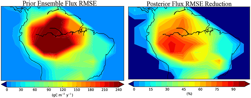
Figure 5. (Left) Prior ensemble annual flux RMSE for the Amazon CO₂ OSSE, which represents a 5% underestimate of annual GPP relative to CASA-GFED. (Right) RMSE reduction after assimilating GeoCarb observations for a single year. This reduction leads to posterior errors of about 75 gC m⁻² y⁻¹ over the Amazon basin. Similar experiments with smaller prior mismatch led to a similar posterior RMSE (not shown), indicating the strong data constraint of GeoCarb observations.

Hypothesis 4: Tropical Amazonian Ecosystems Are a Large (50–100 MtC) Source for CH₄

To test the ability of GeoCarb to detect CH₄ variations, we performed a signal detection experiment using TM5 to propagate different CH₄ emissions into X_CH4 pseudo-observations. TM5 was driven by the surface flask constrained MACC-II CH₄ flux inversion estimates (http://apps.ecmwf.int/datasets/data/macc-ghg-inversions/?version=v10-S1NOAA). The difference between the August emissions for 2011 and 2012 is displayed in Figure 6. Climatologically, the time period in question was a drought for the Amazon, which is believed to increase the outgassing of CH₄ to the atmosphere (Ringeval et al., 2014). The 2011 MACC-II annual Amazon CH₄ emissions were approximately 71 MtC, and the enhancement (2011–2012) for August in the region north of the Amazon was approximately 1.04 MtC. The deficit in the region south of the Amazon was about 0.52 MtC for August. These numbers are within the reported uncertainties (Ringeval et al., 2014).

FIGURE 6

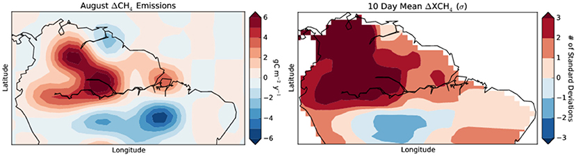
Figure 6. (Left) Difference between 2011 and 2012 emissions for August, which demonstrates the enhanced source in 2012 north of the Amazon, and diminished source south of the Amazon, according to MACC. (Right) The resulting gridded differences in X_CH4 as would be seen from GeoCarb, averaged over 10 days and scaled by the uncertainty. After 10 days, a detectability threshold of 3 standard deviations is achieved for the northern region, and 1–2 standard deviations for the southern region. Longer averaging times of ~20 days led to greater detectability due to daily sampling, even in the presence of clouds.

The difference between the resulting X_CH4 data, normalized by the standard error of the mean for a 10-day average is shown in Figure 6. The elevated emissions north of the Amazon River are detected at a 3σ level, and the reduced emissions south of the Amazon are detected at 1σ level. For longer (20-day) averaging times, the southern is detectable at 3σ as well (not shown). Clearly, Hypothesis 4 can be addressed successfully by the GeoCarb Mission.

Hypothesis 5: The CONUS Methane Emissions Are a Factor 1.6 ± 0.3 Larger Than in the EPA Database

To demonstrate the ability of GeoCarb to address Hypothesis 5, we performed a signal detection experiment using the surface emissions compiled for the Transcom CH₄ intercomparison project (Patra et al., 2011), which contains anthropogenic CH₄ emissions from the Emission Database for Global Atmospheric Research [EDGAR, (Olivier et al., 2005)], as well natural emissions from various other sources, which generally agree with EPA on national scales. We amplified the EDGAR anthropogenic flux component by 1.6 in line with the conclusions of Miller et al. (2013), and the difference between the baseline and enhanced emissions is displayed in Figure 7. There are several hot spots corresponding to natural gas production and mines in the West, South, and Appalachia. Due to the stationarity of these emissions, the model was run with each set of fluxes for 30 days, and then the differences in X_CH4 were examined. These differences, scaled by the uncertainty for a single regional scan, are displayed in Figure 7. Notably, the hot spots are detected at greater than the 2σ level for 1° resolution (the minimum permitted by TM5) with only a single measurement scan. The spatial pattern in the observation differences is a result of atmospheric transport, which smooths spatial gradients. In a real monitoring scenario, multiple days of soundings would be used to isolate the effects of transport in order to estimate emissions.

FIGURE 7

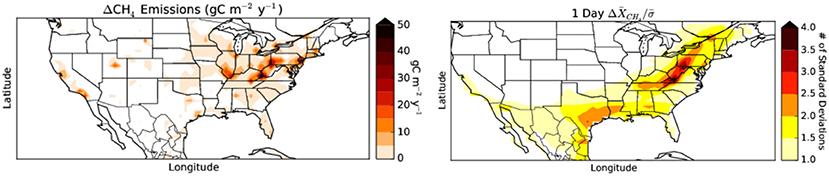
Figure 7. (Left) The emissions difference used for the CONUS fugitive methane experiment, equal to 0.6 times the EDGAR inventory in line with Miller et al. (2013). (Right) The resulting gridded differences in X_CH4 as would be seen from a single GeoCarb daily scan after 30 days of transport, averaged over 100 km and scaled by the uncertainty. The role of atmospheric transport is evident in the figure, as the spatial signatures are diffused by the atmosphere.

The coarse resolution permitted by TM5 is not the model production system planned for use with the extremely high volume of GeoCarb observations. Current efforts are underway to develop chemical tracer transport models and data assimilation techniques that will use GeoCarb data at their native resolution as well as incorporating the state of the art in numerical weather prediction information.

Hypothesis 6: Larger Cities Are More Emissions Efficient Than Smaller Ones

To test this hypothesis, we must be able to estimate the CO₂ emissions from cities over a wide range of populations (at least one order of magnitude). By extending the calculations of Rayner et al. (2014), we estimate the posterior flux uncertainties for an idealized urban geometry and notional concentration uncertainties. Here we use, as an example, urban geometry corresponding to the megalopolis of Mexico City. As always for a flux inversion OSSE, the three ingredients are (1) prior errors in the emissions, (2) errors in the concentrations, and (3) an observation operator mapping emissions to concentrations. Again, following our earlier work, we estimate emissions on a 5 × 5 km grid. The diurnal cycle is subdivided into 4 periods. Reflecting the annual nature of the hypothesis, we solve for monthly averaged fluxes. Emission uncertainties are set at 25% of the emissions. These emissions, in turn, are derived from the 1 km version of the fossil fuel emission aggregated to 5 × 5 km. Sampling density is set by assuming 3 scans of the notional Mexico City location each day at 8 a.m., midday and 4 p.m. We assume that 10% of available soundings yield usable retrievals, a conservative assumption consistent with highly polluted environments. The observation operator is provided by the statistical SatPlume model, which models the development of tracer plumes from point sources according to the advection of the plume's centroid and its three-dimensional spread (Rayner et al., 2014). The resulting tracer distributions are sampled consistently with the viewing geometry and weighting function of the retrieval. These OSSEs use both CO₂ and CO measurements.

We test the hypothesis by calculating the slope of emissions vs. size. We calculate the uncertainty of emissions for 10 fictitious cities. Each city has the same geometry as Mexico City but emissions scaled from 10 to 100% of the nominal value in steps of 10%. Because the emission prior uncertainties are set at 25% of emissions, the prior uncertainty grows with the emissions from the city. We calculate the slope of emissions vs. size using standard weighted least squares. The uncertainties in the emissions imply an uncertainty in this slope. This uncertainty must be small enough to falsify the linear hypothesis for the prior emissions; this uncertainty is 19%. Without observations, this is insufficient to separate the linear hypothesis of Fragkias et al. (2013) from the scaling law of 1.15 proposed by Bettencourt (2013).

The inversion, however, reduces the uncertainty in the total emissions. Reductions are larger for larger emissions, ranging from 33% for Mexico City case down to only 2% for a city with one tenth these emissions. This also improves our confidence in the slope of emissions vs. size which now has an uncertainty of 12%. This is already enough to meaningfully separate the two hypotheses, and this separation would greatly increase with a full year of data vs. 1 month.

Conclusions and Future Work

By carefully connecting measurement requirements to flux uncertainties, we have demonstrated the potential for GeoCarb to revolutionize our understanding of the carbon cycle using the OSSEs detailed above. Though these experiments are not exhaustive explorations of the scientific capabilities of GeoCarb, they address the goals of the mission, i.e., quantifying urban and regional scale CO₂ emissions, diagnosing GPP through SIF, and better understanding the biogenic and anthropogenic sources of CH₄. Importantly, the OSSEs make this demonstration in the presence of uncertainties derived using existing validated observations from space, i.e., albedos from MODIS and cloud and aerosol statistics from CALIPSO. With more OSSEs planned in the period leading up to launch, we will quantify the impacts of imperfect knowledge of clouds and aerosols in terms of measurement bias, and the corresponding impact on flux estimates through regional scale OSSEs. By leveraging these simulation experiments as well as the lessons learned from OCO-2, GeoCarb will be able to make the leap from launch to science.

Existing unpublished work (Crowell et al, in preparation) suggests that three geostationary satellites with strategic placements [e.g., over the Americas (~85°W), Africa (~70°E), and Tropical Asia (~110°E)] as well as a passive Low Earth Orbiter with a wide swath would be sufficient to constrain the carbon cycle across scales from urban to the globe. Further exploration of the use of a constellation of satellites, particularly with different systematic errors, is crucial for better understanding the potential of such an approach (Sellers et al., 2015, 2018).

Author James Lemen is employed by Lockheed Martin Advanced Technology Center. Author Igor Polonsky is employed by Atmospheric and Environmental Research. Author Jack Kumer is deceased. All other authors declare no competing interests.

Author Contributions

BM wrote and edited the manuscript. SC performed the regional simulations, wrote, and edited the manuscript. PR performed urban simulations, wrote, and edited the manuscript. JK performed the instrument modeling. CO and IP performed retrieval simulations. DO performed retrieval simulations, wrote, and edited the manuscript. SU performed urban flux retrievals. DS provided guidance on carbon cycle dynamics. JL provided instrument guidance.

Funding

Funding for SC is provided by NASA under awards NNX15AJ37G and 80LARC17C0001.

Conflict of Interest Statement

The authors declare that the research was conducted in the absence of any commercial or financial relationships that could be construed as a potential conflict of interest.

References

Alvarez, R. A., Zavala-Araiza, D., Lyon, D. R., Allen, D. T., Barkley, Z. R., Brandt, A. R., et al. (2018). Assessment of methane emissions from the U.S. Oil and gas supply chain. Science 361, 186–188. doi: 10.1126/science.aar7204

PubMed Abstract | CrossRef Full Text | Google Scholar

Andres, R. J., Boden, T. A., and Marland, G. (2015). Monthly Fossil-Fuel CO2 Emissions: Mass of Emissions Gridded by One Degree Latitude by One Degree Longitude. Oak Ridge, TN: U.S. Department of Energy; Carbon Dioxide Information Analysis Center, Oak Ridge National Laboratory.

Babenhauserheide, A., Basu, S., Houweling, S., Peters, W., and Butz, A. (2015). Comparing the carbontracker and TM5-4DVar data assimilation systems for CO₂ surface flux inversions. Atmos. Chem. Phys. 15, 9747–9763. doi: 10.5194/acp-15-9747-2015

CrossRef Full Text | Google Scholar

Baker, D. F., Bösch, H., Doney, S. C., O'Brien, D., and Schimel, D. S. (2010). Carbon source/sink information provided by column CO₂ measurements from the Orbiting Carbon Observatory. Atmos. Chem. Phys. 10, 4145–4165. doi: 10.5194/acp-10-4145-2010

CrossRef Full Text | Google Scholar

Baker, I., Denning, A. S., Hanan, N., Prihodko, L., Uliasz, M., Vidale, P., et al. (2003). Simulated and observed fluxes of sensible and latent heat and CO₂ at the WLEF-TV tower using SiB2.5. Glob. Change Biol. 9, 1262–1277. doi: 10.1046/j.1365-2486.2003.00671.x

CrossRef Full Text | Google Scholar

Basu, S., Guerlet, S., Butz, A., Houweling, S., Hasekamp, O., Aben, I., et al. (2013). Global CO₂ fluxes estimated from GOSAT retrievals of total column CO₂. Atmos. Chem. Phys. 13, 8695–8717. doi: 10.5194/acp-13-8695-2013

CrossRef Full Text | Google Scholar

Bettencourt, L. M. (2013). The origins of scaling in cities. Science 340, 1438–1441. doi: 10.1126/science.1235823

PubMed Abstract | CrossRef Full Text | Google Scholar

Bloom, A. A., Lauvaux, T., Worden, J., Yadav, V., Duren, R., Sander, S. P., et al. (2016). What are the greenhouse gas observing system requirements for reducing fundamental biogeochemical process uncertainty? Amazon wetland CH₄ emissions as a case study. Atmos. Chem. Phys. 16, 15199–15218. doi: 10.5194/acp-16-15199-2016

CrossRef Full Text | Google Scholar

Brandt, A. R., Heath, G. A., and Cooley, D. (2016). Methane leaks from natural gas systems follow extreme distributions. Environ. Sci. Technol. 50, 12512–12520. doi: 10.1021/acs.est.6b04303

PubMed Abstract | CrossRef Full Text | Google Scholar

Chevallier, F., Ciais, P., Conway, T. J., Aalto, T., Anderson, B. E., Bousquet, P., et al. (2010). CO₂ surface fluxes at grid point scale estimated from a global 21 year reanalysis of atmospheric measurements. J. Geophys. Res. 115:D21307. doi: 10.1029/2010JD013887

CrossRef Full Text | Google Scholar

Cox, P. M., Betts, R. A., Jones, C. D., Spall, S. A., and Totterdell, I. J. (2000). Acceleration of global warming due to carbon-cycle feedbacks in a coupled climate model. Nature 408, 184–187. doi: 10.1038/35041539

PubMed Abstract | CrossRef Full Text | Google Scholar

Crowell, S. M. R., Randolph Kawa, S., Browell, E. V., Hammerling, D. M., Moore, B., Schaefer, K., et al. (2018). On the ability of space-based passive and active remote sensing observations of CO₂ to detect flux perturbations to the carbon cycle. J. Geophys. Res. Atmos. 123, 1460–1477. doi: 10.1002/2017JD027836

CrossRef Full Text | Google Scholar

Damm, A., Kneubühler, M., Schaepman, M. E., and Rascher, U. (2012). Evaluation of gross primary production (GPP) variability over several ecosystems in Switzerland using sun-induced chlorophyll fluorescence derived from APEX data in 2012 IEEE International Geoscience and Remote Sensing Symposium (Munich), 7133–7136.

Google Scholar

de Viesa, W., Solbergb, S., Dobbertinc, M., Sterbad, H., Laubhannd, D., van Oijene, M., et al. (2009). The impact of nitrogen deposition on carbon sequestration by European forests and heathlands. Forest Ecol. Manage. 258, 1814–1823. doi: 10.1016/j.foreco.2009.02.034

CrossRef Full Text | Google Scholar

Dee, D. P., Uppala, S., Simmons, A., Berrisford, P., Poli, P., Vitart, F., et al. (2011). The ERA-interim reanalysis: configuration and performance of the data assimilation system. Quart. J. R. Meteorol. Soc. 137, 553–597. doi: 10.1002/qj.828

CrossRef Full Text | Google Scholar

Doney, S. C., Lima, I., Feely, R. A., Glover, D. M., Lindsay, K., Wanninkhof, R., et al. (2009). Mechanisms governing interannual variability in upper-ocean inorganic carbon system and air-sea CO₂ fluxes: physical climate and atmospheric dust. Deep Sea Res. Part II 56, 640–655. doi: 10.1016/j.dsr2.2008.12.006

CrossRef Full Text | Google Scholar

Eldering, A., Wennberg, P. O., Crisp, D., Schimel, D. S., Gunson, M. R., Chatterjee, A., et al. (2017). The orbiting carbon observatory-2 early science investigations of regional carbon dioxide fluxes. Science 358:eaam5745. doi: 10.1126/science.aam5745

PubMed Abstract | CrossRef Full Text | Google Scholar

Fragkias, M., Lobo, J., Strumsky, D., and Seto, K. C (2013). Does size matter? Scaling of CO₂ emissions and urban areas. PLoS ONE 8:e64727. doi: 10.1371/journal.pone.0064727

PubMed Abstract | CrossRef Full Text | Google Scholar

Frankenberg, C., Fisher, J. B., Worden, J., Badgley, G., Saatchi, S., et al. (2011). New global observations of the terrestrial carbon cycle from GOSAT: patterns of plant fluorescence with gross primary productivity. Geophys. Res. Lett. 38:L17706. doi: 10.1029/2011GL048738

CrossRef Full Text | Google Scholar

Frankenberg, C., O'Dell, C., Berry, J., Guanter, L., Joiner, J., Köhler, P., et al. (2014). Prospects for chlorophyll fluorescence remote sensing from the orbiting carbon observatory-2. Remote Sens. Environ. 147, 1–12. doi: 10.1016/j.rse.2014.02.007

CrossRef Full Text | Google Scholar

Frankenberg, C., Platt, U., and Wagner, T. (2005): Iterative maximum a posteriori (IMAP)-DOAS for retrieval of strongly absorbing trace gases: model studies for CH4 CO₂ retrieval from near infrared spectra of SCIAMACHY onboard ENVISAT. Atmos. Chem. Phys. 5, 9–22. doi: 10.5194/acp-5-9-2005

CrossRef Full Text

Friedlingstein, P., Meinshausen, M., Arora, V. K., Jones, C. D., Anav, A., Liddicoat, S. K., et al. (2014). Uncertainties in CMIP5 climate projections due to carbon cycle feedbacks. Climate J. 27, 511–526. doi: 10.1175/JCLI-D-12-00579.1

CrossRef Full Text | Google Scholar

Guanter, L., Zhang, Y., Jung, M., Joiner, J., Voigt, M., Berry, J., et al. (2014). Global and time-resolved monitoring of crop photosynthesis with chlorophyll fluorescence. Proc. Natl. Acad. Sci. U.S.A. 111, E1327–E1333. doi: 10.1073/pnas.1320008111

PubMed Abstract | CrossRef Full Text | Google Scholar

Houghton, R. A. (2000). Interannual variability in the global carbon cycle. J. Geophys. Res. 105, 20121–20130. doi: 10.1029/2000JD900041

CrossRef Full Text | Google Scholar

Houweling, S., Baker, D., Basu, S., Boesch, H., Butz, A., Chevallier, F., Zhuravlev, R., et al. (2015). An intercomparison of inverse models for estimating sources and sinks of CO₂ using GOSAT measurements. J. Geophys. Res. Atmos. 120, 5253–5266. doi: 10.1002/2014JD022962

CrossRef Full Text | Google Scholar

Kirschke, S., Bousquet, P., Ciais, P., Saunois, M., Canadell, J. G., et al. (2013). Three decades of global methane sources and sinks (2013). Nat. Geosci. 6, 813–823. doi: 10.1038/ngeo1955

CrossRef Full Text | Google Scholar

Kondo, M., Ichii, K., Takagi, H., and Sasakawa, M. (2015). Comparison of the data-driven top-down and bottom-up global terrestrial CO₂ exchanges: GOSAT CO₂ inversion and empirical eddy flux upscaling. J. Geophys. Res. Biogeosci. 120, 1226–1245. doi: 10.1002/2014JG002866

CrossRef Full Text | Google Scholar

Krol, M., Houweling, S., Bregman, B. M, van den, Broek, Segers, A., van Velthoven, P., et al. (2005). The two-way nested global chemistry-transport zoom model TM5: algorithm and applications. Atmos. Chem. Phys. 5, 417–432. doi: 10.5194/acp-5-417-2005

CrossRef Full Text | Google Scholar

Kulawik, S., Wunch, D., O'Dell, C., Frankenberg, C., Reuter, M., Oda, T., et al. (2016). Consistent evaluation of ACOS-GOSAT, BESD-SCIAMACHY, CarbonTracker, and MACC through comparisons to TCCON. Atmos. Measure. Techn. 9, 683–709. doi: 10.5194/amt-9-683-2016

CrossRef Full Text | Google Scholar

Le Quéré, C., Andrew, R. M., Friedlingstein, P., Sitch, S., Pongratz, J., Manning, A. C., et al. (2018). Global carbon budget 2017. Earth Syst. Sci. Data 10, 405–448. doi: 10.5194/essd-10-405-2018

CrossRef Full Text | Google Scholar

Maksyutov, S., Takagi, H., Valsala, V. K., Saito, M., Oda, T., Saeki, T., et al. (2013). Geoscientific instrumentation methods and data systems regional CO₂ flux estimates for 2009–2010 based on GOSAT and ground-based CO₂ observations. Atmos. Chem. Phys. 13, 9351–9373. doi: 10.5194/acp-13-9351-2013

CrossRef Full Text | Google Scholar

Massart, S., Agusti-Panareda, A., Aben, I., Butz, A., Chevallier, F., Crevoisier, C., et al. (2014). Assimilation of atmospheric methane products into the MACC-II system: from SCIAMACHY to TANSO and IASI. Atmos. Chem. Phys. 14, 6139–6158. doi: 10.5194/acp-14-6139-2014

CrossRef Full Text | Google Scholar

Miller, S. M., Wofsy, S. C., Michalak, A. M., Kort, E. A., Andrews, A. E., Biraud, S. C., et al. (2013). Anthropogenic emissions of methane in the United States. Proc. Natl. Acad. Sci. U.S.A. 110, 20018–20022. doi: 10.1073/pnas.1314392110

PubMed Abstract | CrossRef Full Text | Google Scholar

Nelson, R. (2015). The Impact of Aerosols on Space-Based Retrievals of Carbon Dioxide. MSc. thesis, Colorado State University.

Norton, A. J., Rayner, P. J., Koffi, E. N., and Scholze, M. (2018). Assimilating solar-induced chlorophyll fluorescence into the terrestrial biosphere model BETHY-SCOPE v1.0: model description and information content. Geosci. Model Dev. 11, 1517–1536. doi: 10.5194/gmd-11-1517-2018

CrossRef Full Text | Google Scholar

O'Brien, D. M., Polonsky, I. N., Utembe, S. R., and Rayner, P. J. (2016). Potential of a geostationary geoCARB mission to estimate surface emissions of CO₂, CH₄ and CO in a polluted urban environment: case study Shanghai. Atmos. Meas. Tech. 9, 4633–4654. doi: 10.5194/amt-9-4633-2016

CrossRef Full Text | Google Scholar

O'Dell, C. W., Connor, B., Bösch, H., O'Brien, D., Frankenberg, C., Castano, R., et al. (2012). The ACOS CO₂ retrieval algorithm – Part 1: description and validation against synthetic observations. Atmos. Meas. Tech. 5, 99–121. doi: 10.5194/amt-5-99-2012

CrossRef Full Text | Google Scholar

O'Dell, C. W., Eldering, A., Wennberg, P. O., Crisp, D., Gunson, M. R., Fisher, B., et al. (2018). Improved Retrievals of Carbon Dioxide from the Orbiting Carbon Observatory-2 with the version 8 ACOS algorithm. Atmos. Meas. Tech. Discuss. doi: 10.5194/amt-2018-257 [Epub ahead of print].

CrossRef Full Text | Google Scholar

Olivier, J. G. J., Van Aardenne, J. A., Dentener, F., Pagliari, V., Ganzeveld, L. N.J., and Peters, A. H. W. (2005). Recent trends in global greenhouse gas emissions: regional trends 1970-2000 and spatial distribution of key sources in 2000. Env. Sci. 2, 81–99. doi: 10.1080/15693430500400345

CrossRef Full Text | Google Scholar

Palmer, P. I., Suntharalingam, P., Jones, D. B. A., Jacob, D. J., Streets, D. G., Fu, Q., et al. (2006). Using CO₂ :CO correlations to improve inverse analyses of carbon fluxes. J. Geophys. Res. 111:D12318. doi: 10.1029/2005JD006697

CrossRef Full Text | Google Scholar

Patra, P. K., Houweling, S., Krol, M., Bousquet, P., Belikov, D., Bergmann, D., Wilson, C., et al. (2011). TransCom model simulations of CH4 and related species: linking transport, surface flux and chemical loss with CH4 variability in the troposphere and lower stratosphere. Atmos. Chem. Phys. 1124, 12813–12837. doi: 10.5194/acp-11-12813-2011

CrossRef Full Text | Google Scholar

Peters, W., Jacobson, A. R., Sweeney, C., Andrews, A. E., Conway, T. J., Masarie, K., et al. (2007). An atmospheric perspective on North American carbon dioxide exchange: carbontracker. Proc. Natl. Acad. Sci. U.S.A. 104, 18925–18930. doi: 10.1073/pnas.0708986104

PubMed Abstract | CrossRef Full Text | Google Scholar

Polonsky, I. N., O'Brien, D. M., Kumer, J. B., and O'Dell, C. W. (2014). Performance of a geostationary mission, geoCARB, to measure CO₂, CH₄ and CO column-averaged concentrations. Atmos. Meas. Tech. 7, 959–981. doi: 10.5194/amt-7-959-2014

CrossRef Full Text | Google Scholar

Potter, C. S., Randerson, J. T., Field, C. B., Matson, P. A., Vitousek, P. M., et al. (1993). Terrestrial ecosystem production – A process model based on global satellite and surface data. Global Biogeochem. Cycles 7, 811–841. doi: 10.1029/93GB02725

CrossRef Full Text | Google Scholar

Rayner, P. J., Law, R. M., Allison, C. E., Francey, R. J., Trudinger, C. M., and Pickett-Heaps, C. (2008). Interannual variability of the global carbon cycle (1992–2005) inferred by inversion of atmospheric CO2 and δ13CO2 measurements. Global Biogeochem. Cycles 22:GB3008. doi: 10.1029/2007GB003068

CrossRef Full Text | Google Scholar

Rayner, P. J., and O'Brien, D. M. (2001). The utility of remotely sensed CO₂ concentration data in surface source inversions. Geophys. Res. Lett. 28, 175–178. doi: 10.1029/2000GL011912

CrossRef Full Text | Google Scholar

Rayner, P. J., Utembe, S. R., and Crowell, S. (2014). Constraining regional greenhouse gas emissions using geostationary concentration measurements: a theoretical study. Atmos. Measure. Techn. 7, 3285–3293. doi: 10.5194/amt-7-3285-2014

CrossRef Full Text | Google Scholar

Ringeval, B., Houweling, S., van Bodegom, P. M., Spahni, R., van Beek, R., et al. (2014). Methane emissions from floodplains in the amazon basin: challenges in developing a process-based model for global applications. Biogeosciences 11, 1519–1558. doi: 10.5194/bg-11-1519-2014

CrossRef Full Text | Google Scholar

Schimel, D., Stephens, B. B., and Fisher, J. B. (2015). Effect of increasing CO2 on the terrestrial carbon cycle. Proc. Natl. Acad. Sci.U.S.A. 112, 436–441. doi: 10.1073/pnas.1407302112

PubMed Abstract | CrossRef Full Text | Google Scholar

Sellers, P., Moore, B., Schimel, D., Baker, D., Berry, J., Bowman, K., et al. (2015). An Advance Planning Pre-decadal Survey Workshop: The Carbon-Climate System. Workshop Report: Availanble online at: http://cce.nasa.gov/cce/pdfs/final_carbon_climate.pdf

Google Scholar

Sellers, P. J., Schimel, D. S., Moore, B., Liu, J., and Eldering, A. (2018). Observing carbon cycle–climate feedbacks from space. Proc. Natl. Acad. Sci. U.S.A. 115, 7860–7868. doi: 10.1073/pnas.1716613115

PubMed Abstract | CrossRef Full Text | Google Scholar

Sitch, S., Smith, B., Prentice, I. C., Arneth, A., Bondeau, A., Cramer, W., et al. (2003). Evaluation of ecosystem dynamics, plant geography and terrestrial carbon cycling in the LPJ dynamic global vegetation model. Glob. Change Biol. 9,161–185 doi: 10.1046/j.1365-2486.2003.00569.x

CrossRef Full Text | Google Scholar

Stocker, T. F., Qin, D., Plattner, G. K., Tignor, M., Allen, S. K., Boschung, J., et al. (Eds).. (2013). IPCC, 2013, Climate Change 2013: The Physical Science Basis in Contribution of Working Group I to the Fifth Assessment Report of the Intergovernmental Panel on Climate Change, Chapter 6 (Cambridge; New York, NY: Cambridge University Press), 1535.

Google Scholar

Takahashi, T., Sutherland, S. C., Wanninkhof, R., Sweeney, C., Feely, R. A., Bates, N., et al. (2009). Climatological mean and decadal changes in surface ocean CO₂, and Net Sea-Air CO₂ flux over the global oceans. Deep Sea Res. 56, 554–577. doi: 10.1016/j.dsr2.2008.12.009

CrossRef Full Text | Google Scholar

Taylor, T. E., O'Dell, C. W., O'Brien, D. M., Kikuchi, N., Yokota, T., Nakajima, T. Y., et al. (2012). Comparison of cloud- screening methods applied to GOSAT near-infrared spectra. IEEE Trans. GeoSci. Remote Sens. 50, 295–309. doi: 10.1109/TGRS.2011.2160270

CrossRef Full Text | Google Scholar

van der Werf, G. R., Randerson, J. T., Giglio, L., Collatz, G. J., Mu, M., Kasibhatla, P. S., et al. (2010). Global fire emissions and the contribution of deforestation. Agriculture, and Peat Fires (1997-2009). Atmos. Chem. Phys. 10, 11707–11735. doi: 10.5194/acp-10-11707-2010

CrossRef Full Text | Google Scholar

Wang, J. S., Kawa, S. R., James Collatz, G., Sasakawa, M., Gatti, L. V., Machida, T., et al. (2018). A global synthesis inversion analysis of recent variability in CO₂ fluxes using GOSAT and in situ observations. Atmos. Chem. Phys. 18, 11097–11124. doi: 10.5194/acp-18-11097-2018

CrossRef Full Text | Google Scholar

Wunch, D., Wennberg, P. O., Osterman, G., Fisher, B., Naylor, B., Roehl, M. C., et al. (2017). Comparisons of the Orbiting Carbon Observatory-2 (OCO-2) XCO₂ measurements with TCCON. Atmos. Measure. Tech. 10, 2209–2238. doi: 10.5194/amt-10-2209-2017

CrossRef Full Text | Google Scholar

Yan, Y., Luo, Y., Zhou, X., and Chen, J. (2014). Sources of variation in simulated ecosystem carbon storage capacity from the 5th Climate Model Intercomparison Project (CMIP5). Tellus B. 66. doi: 10.3402/tellusb.v66.22568

CrossRef Full Text | Google Scholar