Multi-Scale Phenology of Temperate Grasslands: Improving Monitoring and Management With Near-Surface Phenocams

Introduction

Grasslands represent one of the most dynamic and widespread biomes on Earth are the dominant ecosystems in a variety of climatic conditions (Scurlock and Hall, 1998). However, despite their importance in grazing systems and their acknowledged provision of ecosystem services, historical, and ongoing land management practices have degraded grasslands throughout the world (Ceballos et al., 2010). This is particularly true for temperate grasslands, which are facing many threats to their sustainable future, including modification for agriculture, habitat fragmentation, weed invasions, and changes in species composition due to a changing climate (Peart, 2008).

In Australia's temperate Southern Tablelands region, grasslands support both unique native flora and an important grazing industry. Grazing favors a community shift from tall perennial grasses to short grasses, and fertilization favors exotic annuals over native perennials (Moore and Biddiscombe, 1964; Gott et al., 2015). Historical land use of the Southern Tablelands therefore drives a patchwork of grasslands dominated by a variety of native grasses, exotic pasture grasses, invasive weeds, or a continuum of intermediate states. These grasslands differ greatly in their composition, structure, and functional attributes (Benson, 1994). Many native temperate grassland communities are only present as remnants and occupy a small fraction of their pre-European range (Groves, 1979; Benson, 1994). Their conservation and restoration is recognized as a priority, however there is an acute need to integrate conservation and agricultural values to ensure success (Wong and Dorrough, 2015). Classification of grasslands based on these attributes is the first step in being able to determine appropriate ecological and agricultural management.

Data for effective classification can be provided through field surveys, however these can be labor-intensive and impractical on a large scale. As an alternative, remote sensing has been explored as a potential approach to identify grassland types and condition. Efforts to discriminate grassland communities have had some success both worldwide (e.g., Price et al., 2002) and within Australia (Hill et al., 1999; Agrecon, 2004; Lymburner et al., 2011), though the classification groupings can be broad. Achieving finer-scale classification of temperate grasslands remains challenging due to their dynamic, heterogeneous nature (Hill, 2013), habit of retaining dead material on the plant (Tremont and McIntyre, 1994; Morgan and Lunt, 1999), unique shading issues (Shimada et al., 2012), and the continuum between disturbed and undisturbed conditions (Psomas, 2008).

While many factors can be used to classify grassland vegetation, the distinction between C₃ (cool season) or C₄ (warm season) photosynthetic types is fundamental (Epstein et al., 1997; Still et al., 2003; Adjorlolo et al., 2012). The nature of C₃ or C₄ dominance dictates patterns of growth and productivity during different times of the year; C₃ species are more productive in cooler, mesic climates, whereas C₄ species have a greater advantage in warmer and drier regions (Wand et al., 1999; Baldocchi, 2011). In the Australian Southern Tablelands, a continuum occurs from C₃-dominated to C₄-dominated grasslands without any defined spatial distribution. Much of the grassland composition depends as much on disturbance factors (e.g., grazing) as climate (Wimbush and Costin, 1979; Benson, 1994). There is a high uncertainty about how C₃ and C₄ vegetation will respond to increased CO₂ concentration and temperature and to modified moisture regimes predicted in a changing climate (Baldocchi, 2011; IPCC, 2014), in particular how this will impact agricultural productivity (Winslow et al., 2003; Howden et al., 2008; Cullen et al., 2009; Pau et al., 2013). Rising temperatures and lower available moisture are expected to favor C₄ grasses, while higher CO₂ concentrations should favor C₃ grasses (Morgan et al., 2011).

Differentiating C₃-dominant from C₄-dominant grasslands has been a prominent theme in remote sensing research due to distinct C₃/C₄ seasonal productivity patterns (Wang et al., 2013; Dye et al., 2016). Satellite data products characterize “land surface phenology” of vegetation types across landscape to global spatial scales (de Beurs and Henebry, 2004; Broich et al., 2015). These typically use a time-series of vegetation indices calculated from measured spectral reflectance, which can reliably estimate biophysical parameters such as biomass and vegetation cover for a diverse range of vegetation types (Weiser et al., 1986; Huete et al., 2002). Several satellite-based phenology studies include grasslands (Justice and Hiernaux, 1986; Fontana et al., 2008; Cui et al., 2012; Horion et al., 2013; Wang et al., 2013), though the majority of these focus on northern hemisphere grasslands where phenology is strongly driven by temperature. One notable study from southeastern Australia provided a classification of pastures types using Advanced Very High Resolution Radiometer (AVHRR) time-series data (Hill et al., 1999). This study successfully grouped broad land use types (e.g., native pastures, sown pastures, mixed pastures/cropping, and forest) based on similar time-series phenology profiles. More recent landscape-scale phenological research in Australia focuses on arid and semi-arid regions where vegetation dynamics are primarily driven by rainfall (Ma et al., 2013; Petus et al., 2013). The unique vegetation dynamics in many Australian environments (e.g., missing an annual growing season or having multiple greening periods) result in non-seasonal behavior and requires the development of different phenological approaches than those used in typical northern hemisphere systems (Zhang X. et al., 2006; Broich et al., 2015).

Satellite remote sensing has the advantage of capturing large areas consistently, but its usefulness in phenological studies is constrained by temporal (i.e., time of satellite revisit) and spatial resolution (i.e., size of pixel) limitations. In contrast, time-lapse fixed cameras (termed “phenocams”) have no such constraints and have shown great promise in capturing phenological information in a wide range of biomes (Brown et al., 2016), including northern hemisphere broadleaf forest (Ahrends et al., 2008; Richardson et al., 2009; Nagai et al., 2011; Mizunuma et al., 2013), Brazilian cerrado (Alberton et al., 2014), European alpine grasslands (Migliavacca et al., 2011; Julitta et al., 2014), Malaysian tropical forest (Nagai et al., 2016), and grasslands in Japan (Inoue et al., 2015). In Australia, Moore et al. (2016) provided an overview of phenocam imagery captured across the continent at different ecosystems including a tropical rainforest, a tropical savannah and a temperate evergreen forest. Generally, phenocams sample a smaller area than satellites and lack the spectral resolution of modern satellite sensors. However, they have the advantage of capturing high frequency (sub-daily) imagery, they can be positioned to directly monitor the vegetation of interest, atmospheric effects have less impact, and users can visually examine imagery to explain observed data patterns or anomalies. Phenocam imagery is typically converted to a vegetation index such as the Excess Green (e.g., Woebbecke et al., 1995) or the Green Chromatic Coordinate (g_CC) (Gillespie et al., 1987; Sonnentag et al., 2012) through manipulation of the red, green, and blue brightness values. Phenocam-based phenology has shown a good correspondence of phenophase timing when compared with eddy-covariance towers, satellite imagery, and field observations (Richardson et al., 2007; Migliavacca et al., 2011; Nagai et al., 2011; Mizunuma et al., 2013; Toomey et al., 2015; Moore et al., 2017), albeit with quantifiable time lags or restrictions to certain times of year (e.g., remotely sensed observations can be unavailable during the wet-cloudy season).

Remote sensing data is often validated through field biophysical observations (Mutanga and Skidmore, 2004; Zhang Q. et al., 2006; Shen et al., 2008; Liang et al., 2011; Psomas et al., 2011), with some agencies in Australia providing substantial investment and support to this aim (Muir et al., 2011). Some research has shown successful scaling from field measures to remote sensing (e.g., Fisher and Mustard, 2007; Studer et al., 2007). However, others have highlighted the sometimes weak relationship between in situ and satellite observations (Badeck et al., 2004; Ahl et al., 2006; Soudani et al., 2012). One of the more pressing challenges in phenological research is to understand the sources of variability between spatial scales (Friedl et al., 1994; Reed et al., 2009). This is particularly relevant for heterogeneous grasslands, where variability in spatial scales of field measurements can be problematic (Klimeš, 2003).

Given the importance of grasslands for food security and ecosystem preservation and the need for a better understanding of remote sensing-derived phenology over pastures and grasslands, this research aims to:

a) Assess the variability in phenology among of C₃/C₄ temperate grassland types with the use of phenocams;

b) Identify the biophysical drivers that cause changes to grassland land surface phenology;

c) Evaluate the utility of phenocams for capturing temperate grassland phenology; and

d) Compare scales of phenocam phenology data with field measurements and satellite phenology products.

Materials and Methods

Study Sites

The study area is located in the Southern Tablelands region of New South Wales (NSW) and the Australian Capital Territory (ACT), and is part of the South Eastern Highlands bioregion (Environment Australia, 2000). The study area is approximately bounded by the towns of Bungendore (35.2500°S, 149.4500°E), Gungahlin (35.1831°S, 149.1330°E), and Bredbo (35.9420°S, 149.2009°E) (Figure 1). The region has distinct seasonal temperature values (mean monthly ranging from 0 to 30°C) and contains several types of native and exotic grasslands co-occurring within a similar climatic envelope. The climate is characterized by warm summers (December–February) with maximum daily temperatures frequently reaching 35°C. Winters (June–August) are cold, with frequent daily minimum temperatures below 0°C. Rainfall is relatively consistent throughout the year, with a mean of between 30 and 90 mm per month, and an annual average of 650 mm, although rainfall in the region is impacted by elevation, latitude, and aspect and may be spatially sporadic.

FIGURE 1

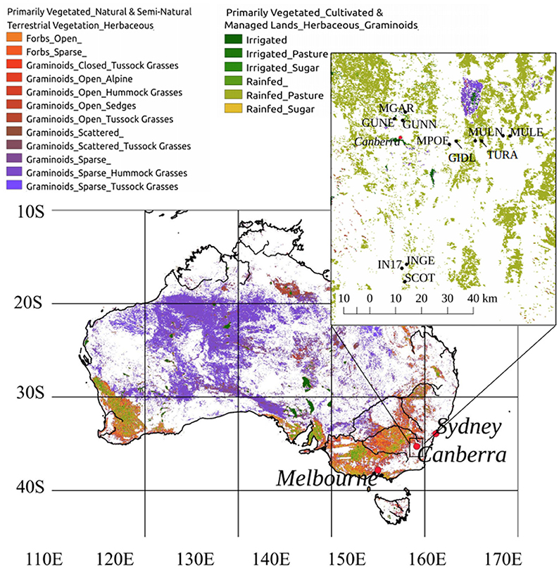
Figure 1. Location of study area, south east of the continent, near the city of Canberra, Australia. Background vegetation mapping refers to the Dynamic Land Cover Dataset (Lymburner et al., 2011). Inset shows the location of individual study sites.

Modeled temperature and rainfall data generated from MODIS Terra Global Land Surface Temperature and Tropical Rainfall Measuring Mission version 7 (data product 3B43-v7) are presented to compare the monthly rainfall and temperature of the study period with the 1998–2017 average (Figures 2A,B). The study period (May 2014–April 2015) had temperatures that were generally consistent with the mean, though the period of December 2014–April 2015 was cooler than average (Figure 2A). Precipitation during the study period was more sporadic; a few months (June December, January and April) had unusually heavy rainfall and many months had lower than average rainfall (Figure 2B).

FIGURE 2

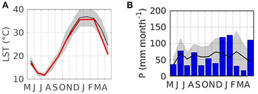
Figure 2. Study site satellite derived climatic variables sampled at Mullunggari Nature Reserve (center pixel) (A) temperature from MODIS Terra Global Land Surface Temperature (LST; °C) (MOD11A2) mean (black line) and standard deviation 1998–2017 (gray area) and this study period (May 2014–April 2015; red line) (B) precipitation (P; mm month-1) from the version 7 Tropical Rainfall Measuring Mission (TRMM) data product (3B43-v7) (0.25 deg) mean (black line) and standard deviation 1998–2017 (gray area) and this study period (May 2014–April 2015; blue bars).

Three replicate areas of four distinct perennial grassland types common to the area were selected. Elevation of the study locations is between 550 and 750m above sea level. Sites were grouped based on the C₃/C₄ and the native/exotic status of the dominant perennial grass species (summarized in Table 1). Site groups were selected based on important grassland types in the region, including those that are used for conservation purposes, and those that are used for grazing agriculture. Sites within each category were not required to have the same dominant species per se, but rather be dominated by the same functional group (e.g., native C₄ grass). This dominance was designated by the terminology used throughout this text as: C₄ Native, C₄ Exotic, C₃ Native, and C₃ Exotic. C₄ Native sites were dominated by the common native grass Themeda triandra, a typical indicator species of low disturbance. C₄ Exotic sites were dominated by the invasive agricultural weed Eragrostis curvula. C₃ Native sites contained a mixture of Austrostipa and Rytidosperma C₃ species typical of grazed native pastures in the region. C₃ Exotic sites were dominated by exotic pasture grasses, typically Phalaris aquatica, Dactylis glomerata, and Festuca arundinaceae. All grassland types contained secondary components of species outside the dominant functional group. For example, C₄ Native sites contained a small fraction of C₃ native grasses and exotic species. C₃ forbs occurred at most site at low vegetative cover.

TABLE 1

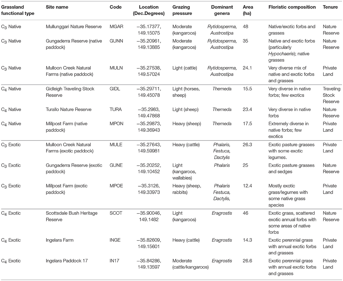
Table 1. Characteristics of study sites by grassland functional type.

All sites met the following criteria: homogenous cover of the selected grassland type; consistent land management throughout the study period; and the grassland area being >20 hectares, with adequate coverage in all dimensions to incorporate satellite pixels. None of the field sites were artificially irrigated.

Time-Lapse Digital Photography

Time-lapse RGB Wingscapes™ cameras (phenocams) in weatherproof housing were installed at each site to capture vegetation changes at a high temporal capacity. The phenocam was mounted 2.3 m above ground level and angled downward ~15° from horizontal. The field-of-view included the horizon in the image but only a small quantity of sky, i.e., most of the scene was the target grassland. This field-of-view captured an area between 2 and 4 hectares. Each camera was positioned to face south to minimize the impacts of sun glint on the images. We collected one image at hourly intervals between 9:00 and 15:00 Australian Eastern Standard Time (UTC +10). No standardization of color was used through the use of reference cards as can be found in similar studies (Ahrends et al., 2008; Richardson et al., 2009; Sonnentag et al., 2012). Color balance drift has been reported in a study using phenocams (Ide and Oguma, 2010) however this only became apparent after 2 years of use. As such, no significant color balance drift is assumed for this study.

The Green Chromatic Coordinate index (g_CC; Equation 1) was used as a surrogate of greenness as it represents the relative brightness of the green fraction compared to the sum of the green, red, and blue bands (Gillespie et al., 1987; Sonnentag et al., 2012). It is a unitless index that pilot studies suggest ranges between 0.25 (no green vegetation) and 0.5 (abundant green vegetation) in the subject grasslands. A variety of phenocam-based studies have preferentially used this index because of its dynamic response to changes in plant biophysical variables and robustness to variations in image brightness due to sky conditions, time of day, or shadowing (Ide and Oguma, 2010; Sonnentag et al., 2012; Julitta et al., 2014).

$\begin{array}{ll}\text{gCC }=\frac{\text{G}}{\text{R}+\text{G}+\text{B}}& (1)\end{array}$

Images were manually filtered and viable images were processed with ImageJ software (Abràmoff et al., 2004) to extract RGB values and calculate g_CC. The mean g_CC across the target area of the image was used for each hourly data point and was used to establish a daily time-series, known as a phenology profile. For some phenocam profiles, we fitted a non-parametric Locally Weighted Scatterplot Smoothing (LOESS) curve to improve visualization and the identification of trends (Cleveland, 1979).

Field Measurements and Floristic Surveys

Monthly biometric measurements included pasture height and vegetation cover using non-destructive methods, and aboveground biomass using destructive harvesting.

• Percent vegetation cover was taken using a point-transect method (NSW Catchment Management Authority, 2005). One 100 m transect was established across a representative part of the study site with cover noted at 1 m intervals. Vegetation cover was classified as: green vegetation (photosynthetic vegetation, PV), dead vegetation (non-photosynthetic vegetation, NPV), and background (bare soil and substrate, BS).

• Average pasture height was measured using a falling plate method (Rayburn and Rayburn, 1998). A standard acrylic plate was mounted on a ruler and allowed to fall on the vegetation at the sample point. The mean value of 20 points was taken.

• Total biomass was harvested within six replicates of 1 m² quadrats to ~1 cm above ground level. The location of each quadrat was randomly selected at each monthly visit without replication. Biomass samples were stored in a plastic bag in a cool environment (a cooler in the field and a refrigerator in the laboratory) prior to processing to prevent degradation. Vegetation was separated into “grasses,” and “forbs” (including pasture legumes, native forbs, and exotic weeds), then further separated into photosynthetic (“green”) and non-photosynthetic (“dead”). Samples were placed in paper bags, oven-dried at 60°C for 72 h and results converted to kg/ha.

Floristic surveys were conducted at each location (three 20 × 20 m plots) each month to monitor species composition. Monthly floristic data is not presented.

Satellite Data Sources

Satellite data were obtained from three sources that represent typical sources of land surface phenology data: the Moderate Resolution Imaging Spectrometer (MODIS) sensor aboard the Terra satellite, the Operational Land Imager (OLI) sensor aboard Landsat 8, and the Enhanced Thematic Mapper Plus (ETM+) sensor on Landsat 7.

The Terra MODIS 16-day composite NDVI (MOD13Q1) at 250 m spatial resolution was downloaded from the NASA Land Processes Distributed Active Archive Center (http://e4ftl01.cr.usgs.gov/) over the period May 1, 2014 to April 30, 2015. The NDVI provided by this product was calculated using the bands specified in Table 2. The data were filtered based on the quality assurance flags provided in the quality control layers of the product, with periods of clouds, high aerosol loads, and low quality were removed. The 16-day composite data reduces impact of cloud cover on long-term data sets, though at the expense of higher temporal resolution. Due to the relatively small size of most of our grassland sites, one pixel (250 × 250 m) was used for analysis.

TABLE 2

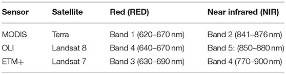
Table 2. Satellite sensor spectral bands used in the calculation of NDVI.

Landsat data (OLI and ETM+) was obtained from the Climate Data Record surface reflectance from the Science Processing Architecture System of USGS Earth Resources Observation and Science Center (http://espa.cr.usgs.gov/), corrected for atmospheric effects and BRDF. We subsequently calculated NDVI from reflectance data as per Equation 2 using the red and near infra-red (NIR) bands specified in Table 2. Landsat 7 and Landsat 8 data were combined into one NDVI time-series as the data have been shown to be equivalent (Li et al., 2014; Ahmadian et al., 2016). The Landsat 7 and 8 data are collected at a nominal 16-day frequency; however this is subject to effects of clouds that can reduce or eliminate the usability of parts of an image. As such, temporal resolution frequently extends beyond 16 days. To capture a similar area as MODIS data sources, we used a 5 × 5 grid of 30 × 30 m Landsat pixels resulting in a total area of 150 × 150 m.

$\begin{array}{ll}\text{NDVI}=\frac{(\text{NIR}-\text{RED})}{(\text{NIR}+\text{RED})}& (2)\end{array}$

On average, there were 19.2 of a possible 23 MODIS 16-day temporal data points for each site (range: 18–20) over the annual study period, and 17.3 Landsat OLI/ETM+ 16-day data points (range: 15–19) of a possible 23. Some large gaps, due primarily to cloud obstruction, were evident in the temporal satellite data which can impact phenology studies, with a maximum 126 day gap for Landsat data and a 48 day gap for MODIS data.

Data processing, including graphical analysis and statistical analysis, was conducted with the R software package (R Core Team, 2013). For quantitative comparison between methods, it was necessary to match data as closely as possible in time. As field sampling was the least frequent data type (monthly), we selected 12 data points from satellite and phenocam time-series that were closest to the 12 field sampling dates (number of days before or after). Pearson's correlations were conducted across all sites using this matched data.

Results

Phenocam Imagery

The phenocam derived g_CC profiles (Figure 3) showed C₃ sites having maximum greenness as a distinct peak in October-November, whereas C₄ sites peaked later (January-February) and showed a broader peak. All sites started greening after August as temperatures warmed which is indicative of the presence of C₃ species (albeit as a secondary component in C₄-dominated sites). C₃ vegetation had a second greening period in late February in response to increased rainfall. Fine-scale vegetation dynamics are observed at all sites as small but rapid increases and decreases in g_CC.

FIGURE 3

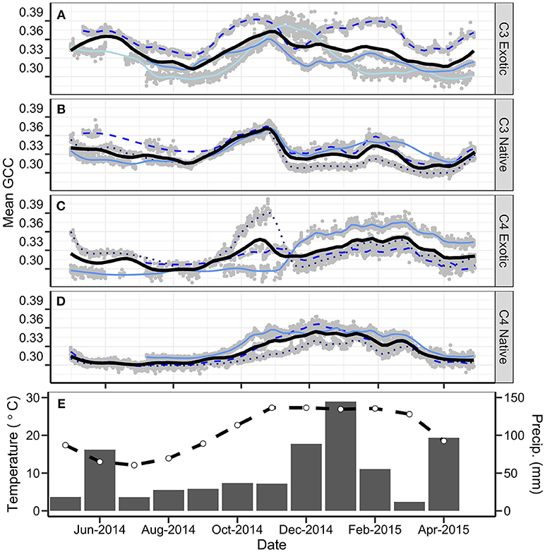
Figure 3. Annual combined g_CC phenology profiles for all sites, grouped by functional type, (A) C₃ Exotic, (B) C₃ Native, (C) C4 Exotic, (D) C4 Native. Gray dots represent hourly data points. Blue lines represent individual sites. The thick black line of each panel is a LOESS fitted curve (span = 0.1) for each functional type. Panel (E) represents the monthly mean maximum temperature (°C; dashed line; Tuggeranong Bureau of Meteorology station) and the monthly rainfall (mm; solid bars; Australian National Botanic Gardens Bureau of Meteorology station) for the study period.

C₃ Exotic grassland sites showed peak greenness in October-November (Figure 3A). However, these sites were variable: one site showed an almost unimodal profile, increasing in g_CC from September, reaching a peak in November, and steadily decreasing to the baseline in January. At the second site we observed green-up steadily climbing to a peak in late October, before decreasing in December. Multiple small increases in g_CC occur until February, followed by a steady decline through March. The third site had two equally dominant peaks in October and February.

The C₃ Native profiles demonstrated a gradual decline of g_CC from May through to August and a characteristic greening pattern commencing in August and reaching a maximum in October-November (Figure 3B). The g_CC then abruptly decreased in November. Patterns changed slightly between the sites from this point; some showed periods of greening and browning through the summer, whereas others had only one small greening period. Two sites showed steady decline in g_CC through February to a minimum in March, whereas the other demonstrated an influence from secondary C₄ species (a low wide peak from December and reaching a minimum in late March).

The C₄ Exotic profiles show consistency in summer peak greenness (January-February) (Figure 3C). The g_CC values were all very low through the winter months, and shared identical timing of the characteristic broad summer peak. The individual sites showed different patterns during spring. One site had a distinctive peak of C₃ vegetation resulting from a flush of spring pasture grasses. Another showed a delayed but very rapid increase in g_CC, commencing in November and lagging biomass-measured greening by 2 months.

The C₄ Native grasslands show a consistent group of profiles (Figure 3D). All sites have low g_CC from May to August, with an indistinct inflection point in late August marking the start of a gradual greening. High g_CC is maintained through January-February followed by a characteristic drop in March as temperatures start to decrease.

Vegetation Cover

All groups showed distinct seasonal changes in cover throughout the year, with the mean time-series presented as Figure 4. The C₄ Native sites demonstrate particularly distinctive and predictable patterns, with low green cover during the winter months, rapid greening in October, and a peak of 75% green cover maintained from December to February. After March, the green cover at C₄ Native sites decreased quickly to 20%. The seasonal green cover variation between C₄ Native sites was low. The C₄ Exotic grasslands display a similar seasonal pattern, though with greater variation between sites: low green cover (~10%) through winter, green-up starting in August with a steady increase to November, and a rapid rise to a peak of 75% in February. C₃ Native sites show a high variability throughout the year, with a peak of 80% green cover in October. Minima in November and March correspond with high temperatures and low rainfall. C₃ Exotic peak green cover is in November (76%) though high green cover is maintained from September through January. The minimum green cover occurs in March for both C₃ Exotic and C₃ Native groups.

FIGURE 4

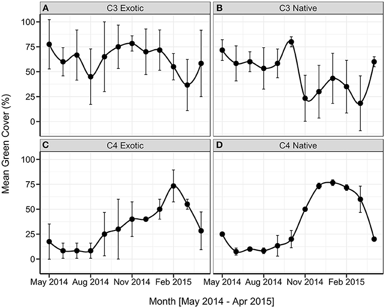
Figure 4. Monthly mean green cover (% ± s.d., n = 3), presented by grassland functional type, (A) C₃ Exotic, (B) C₃ Native, (C) C₄ Exotic, (D) C₄ Native.

Biomass Sampling

Green and dead biomass varied considerably between sites and seasonally at the same location (Figure 5). Exotic groups tended to have the greater quantity of mean green biomass, where we observed the maximum value at a single site of (2,769 kg/ha). The mean green biomass for C₄ Native sites did not exceed 1,000 kg/ha, and C₃ Native sites did not exceed 500 kg/ha. The C₄ Exotic sites had higher green biomass during the summer months than the winter months. By contrast, C₃ Exotic sites fluctuated throughout the year in response to grazing pressures and seasonal drivers, particularly periods of low rainfall. In general, sites that were dominated by C₄ species had low quantities of green biomass during the winter months, though notably still >0. The key features of the C₃ biomass pattern are an increase in September which reaches a peak in November (mean green biomass 1,536 kg/ha for exotic; 586 kg/ha for native). The C₄ sites commenced green-up a month later, in October, and reached a peak in December which was sustained through the summer (1,438 kg/ha exotic; 922 kg/ha native). At two of the three C₄ Exotic sites, we observed an additional peak in late summer (February; mean live biomass 2,026 kg/ha) and hence the associated standard deviation is large.

FIGURE 5

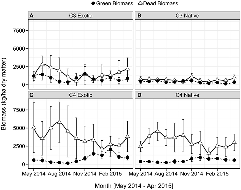
Figure 5. Mean monthly green (solid line) and dead (broken line) biomass (kg/ha ± s.d.; n = 18) by grassland functional type, (A) C₃ Exotic, (B) C₃ Native, (C) C₄ Exotic, (D) C₄ Native.

Dead biomass was greatest in C₄-dominated sites, with a mean maximum of 5,810 kg/ha at exotic C₄ sites and 4,689 at native C₄ sites. This accumulation of dead material was driven by minimal grazing or disturbance at these sites. C₄-dominated sites tended to have a higher biomass during the winter months but exhibited a very high variability between sites and replicates. All C₃ Native sites had a more consistent quantity of dead biomass throughout the year; however, variability was higher between C₃ Exotic sites, hence higher monthly standard deviation. At C₄-dominated sites the dead biomass was much greater than green biomass throughout the year. Forbs contributed a very minor proportion of the overall biomass.

Satellite Data

Satellite phenology profiles are presented as individual sites to allow visualization and comparison of the phenology trends of different satellite greenness products (Figure 6). While the satellite data shows substantial fluctuation, the timing of the maximum NDVI at each site corresponds with the C₃/C₄ functional group.

FIGURE 6

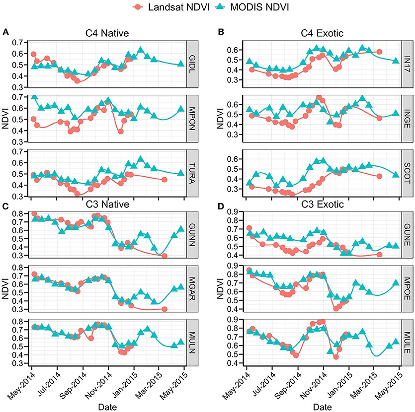
Figure 6. Terra MODIS (▴) and Landsat OLI/ETM+ (•) NDVI data for 1 May 2014–30 April 2015 at (A) C₄ Native sites, (B) C₄ Exotic sites, (C) C₃ Native sites, (D) C₃ Exotic sites.

Landsat and MODIS data at C₄ Native sites (Figure 6A) show similar trends though they deviate substantially in magnitude. The paucity of Landsat data beyond January 2015 due to cloud contamination hindered meaningful comparison. The temporal resolution of C₄ Native seasonal pattern is less clear in satellite data than in other data sources. Two sites (GIDL and TURA) both show a consistently low NDVI below 0.5 throughout the autumn and winter months until green up. After a peak in October, satellite data shows a decrease in greenness toward late November that is not apparent in other data sources. The NDVI increases throughout the remainder of the summer months to a maximum of 0.62 and then slowly tails off toward the winter baseline. By contrast, at the third site (MPON), NDVI is more variable throughout the measurement period, with two peaks evident in October and January.

At C₄ Exotic sites (Figure 6B), Landsat data exhibited smooth trends whereas MODIS fluctuated. Site IN17 showed the most consistency between the two satellite data sources. From a typically low greenness during winter, NDVI started to increase in August to an October peak of 0.6. After a small browning period, NDVI remained relatively high during the summer and decreased to 0.49 by late August. Landsat data for INGE showed a prominent peak in October (NDVI = 0.65), whereas the MODIS peak was apparent in February. Landsat data at SCOT showed a long, gradual increase in NDVI from late August to late December which contrasts with the rapid increase in g_CC observed in the phenocam data. MODIS data at SCOT showed a much more variable signal, with the only clear peak occurring in October and a high NDVI being maintained throughout summer.

The MODIS and Landsat NDVI values for C₃ Native sites (Figure 6C) were comparable, both in magnitude and trend. Most inconsistent data points can be attributed to data gaps. The MODIS data shows consistent temporal patterns with phenocam and biomass trends at all three sites.

Trends of Landsat and MODIS NDVI corresponded well for C₃ Exotic sites (Figure 6D), though deviations in magnitude were particularly evident at one site (GUNE). Like other functional groups, the paucity of Landsat data beyond January 2015 made comparisons difficult. In general, patterns consistent with C₃ characteristics were shown by the satellite data. All three sites showed greening commencing in July–August with a peak in October, and multiple additional peaks in February and April. Two of the C₃ Exotic sites had very high NDVI values, with peak NDVI exceeding 0.8.

Relationship Between Remotely-Sensed and Biophysical Variables

Variables were identified that were expected to be related to the quantity and quality of green vegetation: green grass biomass, green biomass (i.e., grass + forbs), total biomass, green vegetation cover, dead vegetation cover, pasture height, phenocam g_CC, MODIS NDVI, and Landsat NDVI (Figure 7). Correlations are presented across all sites as separation of grassland functional types yielded only minor differences when tested. Longitudinal graphical comparisons of all parameters are presented as Figures 8, 9 for sites GIDL (C₄ Native) and MULN (C₃ Native). These figures are examples of the comparison between phenology variables measured at individual sites.

FIGURE 7

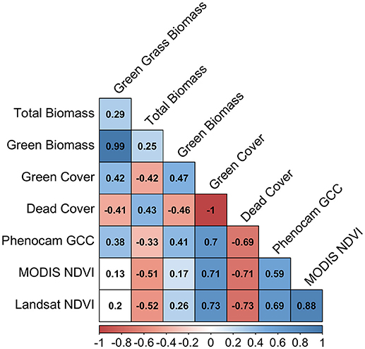
Figure 7. Pearson's correlation of variables across all sites that are relative to quality and quantity of green vegetation. Shaded values represent significant correlation at p = 0.05. Values are Pearson's correlation coefficient (r). Negative values (red) indicate a negative correlation; positive values (blue) indicate a positive correlation.

FIGURE 8

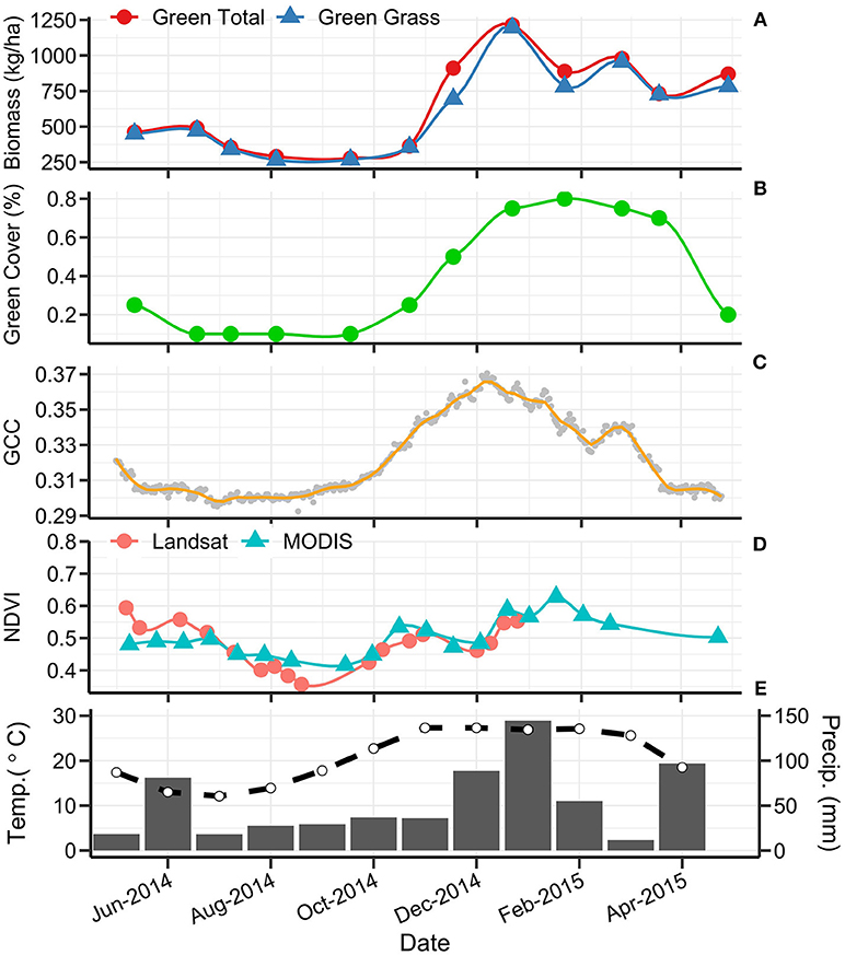
Figure 8. Multi-scale phenology from 1 May 2014 to 30 April 2015 at site GIDL (C₄ Native). From top to bottom panel: (A) total green biomass (•) and green grass biomass (▴) in kg/ha; (B) green cover (%); (C) phenocam 13:00 daily g_CC; (D)Terra MODIS (▴) and Landsat OLI/ETM+ (•) NDVI; (E) monthly mean maximum temperature (°C; dashed line; Tuggeranong Bureau of Meteorology station) and the monthly rainfall (mm; solid bars; Australian National Botanic Gardens Bureau of Meteorology station).

FIGURE 9

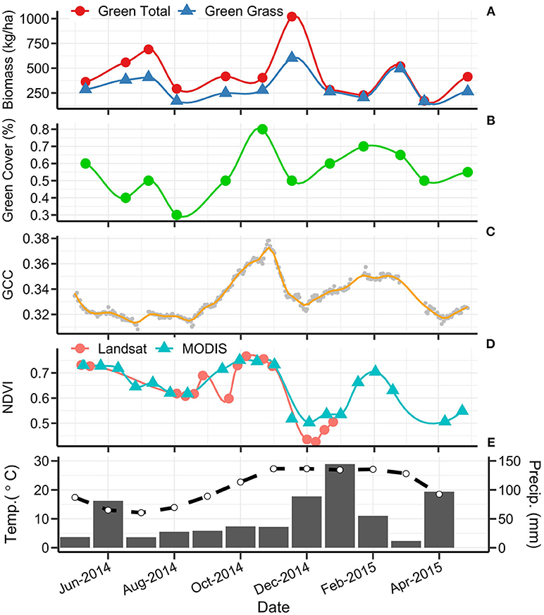
Figure 9. Multi-scale phenology from 1 May 2014 to 30 April 2015 at site MULN (C₃ Native). From top to bottom panel: (A) total green biomass (•) and green grass biomass (▴) in kg/ha; (B) green cover (%); (C) phenocam 13:00 daily g_CC; (D) Terra MODIS (▴) and Landsat OLI/ETM+ (•) NDVI; (E) monthly mean maximum temperature (°C; dashed line; Tuggeranong Bureau of Meteorology station) and the monthly rainfall (mm; solid bars; Australian National Botanic Gardens Bureau of Meteorology station).

Across all sites, green biomass was strongly and significantly correlated with green grass biomass (r = 0.99, p < 0.001). This demonstrates that the biomass was dominated by the influence of grass rather than forbs. Green biomass was poorly-correlated with total biomass (r = 0.25), indicating that the contribution of the dead biomass component has a strong influence on the overall biomass. Green biomass was only weakly correlated with satellite estimates of NDVI (MODIS NDVI r = 0.17; Landsat NDVI r = 0.26). Height was not significantly correlated with green cover, dead cover or phenocam g_CC, and only weakly correlated with satellite and biomass variables.

Phenocam g_CC has a stronger relationship to the fraction of green cover (r = 0.7) than its relationship with any of the biomass variables (green biomass r = 0.41; green grass biomass r = 0.38). A similar strength of correlation is present between green cover and NDVI (Landsat: r = 0.71, MODIS: r = 0.73), with satellite data also having a stronger correlation to green cover than to green biomass (Figure 7). MODIS and Landsat NDVI values are strongly and significantly correlated with one another (r = 0.88, p < 0.001). The correlation between phenocam g_CC and Landsat NDVI (r = 0.69) was stronger than that between g_CC and MODIS NDVI (r = 0.59).

Discussion

Assessment of Phenocams for Monitoring Temperate Grasslands

This research found that the sub-daily image capture available through phenocams allowed for the detection of fine-resolution changes in greenness that were not observed in other methods. Temperate grasslands of the Australian Southern Tablelands show fluctuations in g_CC that represent rapid responses to climatic and environmental change, and phenocams add value for interpreting the dynamics of this vegetation. Changes in phenology due to climate trends typically report differences in scales of days per decade (Parmesan and Yohe, 2003; Badeck et al., 2004; Graham et al., 2009). In many cases, data collected coarser than daily frequency (i.e., satellite and biomass data here presented) will render changes under a certain threshold undetectable. Sampling data at daily frequency also has the capacity to resolve very subtle trends driven by community composition and environmental drivers that are not possible to resolve using other means.

We found the g_CC to be a consistent and repeatable vegetation index for capturing the dynamics of temperate grasslands in the subject region. Similar to other studies (Sonnentag et al., 2012) this index was found to be relatively invariant to changes in illumination. Differences in relative angle between the camera and the target have rarely been explored in the phenocam literature and have the potential to be more confounding on RGB digital numbers and greenness indices than errors associated with illumination effects. Standardization of sensor-target angle is recommended for future studies of groundcover vegetation types.

Phenocams currently lack the spectral resolution shown by many satellites and cannot match their spatial coverage. However, phenocams have enormous potential as tools to support ecological monitoring at an intermediate scale that can reliably estimate biophysical variables at sub-daily frequency. Phenocams may provide advantage to the agricultural sector in determining appropriate times for pasture stocking, mowing, or other management actions. On a larger scale, a network of phenocams could be used to track weed invasions, or report on drought impacts—items that are particularly important to Australian agriculture. As this field develops further, there is a growing need to conduct further testing and analysis in novel biomes, quantify illumination, and camera angle effects on RGB indices, and to promote the standardization of methodology to enable cross-continental phenological comparisons (Brown et al., 2016). These is also significant scope for advances in statistical methods to characterize and analyse time-series imagery (Gray and Song, 2013).

C₃/C₄ Phenological Response

We found C₃/C₄ species composition to be the primary driver of phenology patterns in temperate grasslands of the Australian Southern Tablelands, with several key phenological features identified for C₃- and C₄-dominated grasslands. Some of these features are most prominent in the higher temporal frequency methods (e.g., phenocam g_CC) and are partially obscured by coarser data sources (e.g., MODIS NDVI). Generally in this region C₃-dominated grasslands showed a steady decline in green signal from May to August (austral late autumn/winter). A relatively sharp greening commenced in late August, reaching a peak in late October to early November as C₃ green leaf expansion was at its maximum. Elevated temperatures and low rainfall in November caused a decline in C₃ greenness until secondary greening occurred in late January driven by higher rainfall. In contrast, C₄-dominated grasslands demonstrated a consistently low quantity of green vegetation from May to August. Green-up commenced in September (early spring) and green-up rates tended to be slower than those observed for C₃-dominated vegetation. Major C₄ vegetation greening in October resulted in either a single peak in December (early summer) or consistently high greenness from December through February with a steady return to low green signal in April. The C₄ grasslands exhibited only minor senescence during spring/summer when higher temperatures and low rainfall promoted browning in C₃-dominated systems. The observed patterns were less variable in C₄ than in C₃ grasslands, which may be attributed to a consistent dominant species in the two C₄ grasslands groups.

Comparison of Field and Remotely Sensed Methods

The relationship between phenocam, field, and satellite phenology variables was analyzed using linear correlation, a similar approach to other researchers (e.g., Zhang et al., 2003). We found that green biomass was not-well correlated with total biomass. This stems from the proportionally high contribution of standing litter in some of the subject temperate grasslands, particularly C₄ grasslands that typically retain standing litter throughout the year (Tremont and McIntyre, 1994). The very strong correlation of green biomass to green grass highlights the importance of the grass component for remote sensing: although forbs contribute most to ecosystem species richness in Australian temperate grasslands (Wimbush and Costin, 1979; Tremont and McIntyre, 1994), they contribute a small fraction of total biomass. Green cover was only moderately correlated with green biomass (r = 0.43) but was negatively correlated with total biomass, again stressing the influence of standing litter. This influence of litter may confound attempts to use remote sensing for the classification, management, and monitoring of grasslands in the study region.

Like other grassland studies (e.g., Paruelo et al., 2000; Migliavacca et al., 2011; Inoue et al., 2015), we found a statistically significant relationship between (a) phenocam indices and green biomass and (b) between phenocam indices and satellite NDVI. However, phenocam g_CC was more strongly correlated with green cover than with green biomass and suggests that phenocam data may be more appropriate for estimating cover rather than biomass for Southern Tableland temperate grasslands. Similar research on temperate grasslands in the USA (Vanamburg et al., 2006) suggests that digital camera-based estimates of biomass are poor. However, in European alpine grasslands, Migliavacca et al. (2011) found that their Greenness Index (equivalent to g_CC) was significantly correlated with green biomass and visual greenness estimates. Such inconsistencies between temperate grasslands communities suggest differences the biophysical characteristics of different grassland types and indicate that the more complex the grassland structure, the lower the likely correlation between g_CC and green biomass. As such, results from this study should not be assumed to apply to functionally different temperate grasslands systems, even within Australia.

Green biomass was only weakly correlated with satellite NDVI, contrary to some grassland studies in northern hemisphere biomes (Migliavacca et al., 2011). The abundant standing litter we observed not only obscures green vegetation, but it reflects more light in the red wavelengths, reducing the NDVI signal (Watson et al., 2013). The relatively weak correlation between satellite and ground variables may also be due to data gaps in the satellite time-series and temporal registration between field and satellite data. Overall, we found phenocam g_CC to be better correlated with Landsat NDVI than MODIS NDVI. This may be due to the smaller Landsat footprint and highlights the importance of sampling equivalent size plots for remote sensing comparisons (Rienke and Jones, 2006).

Despite the reasonable correlation between phenocam, satellite and field data, we suggest that a 16-day temporal resolution is too coarse to quantify fine changes that occur in dynamic grassland systems in our study region, particularly given that cloud cover impacts often lengthens this period (Stow et al., 2004). Our phenocam data shows consistent periods of increasing and decreasing greenness over as little as 5 days. Other studies have indicated that an effective 16-day revisit time is insufficient to detect key phenological dates (Westergaard-Nielsen et al., 2013). Daily data products from MODIS are available that can be used to generate finer-scale phenology products (Narasimhan and Stow, 2010), but the temporal resolution comes at a trade-off with data quality (e.g., cloud contamination).

Scale transferability when estimating phenology remains a major challenge (Friedl et al., 1994; Eisfelder et al., 2016). While some studies have reported success in this regard (e.g., Fisher et al., 2006; Fisher and Mustard, 2007), other authors caution that there are still major challenges in scaling biophysical measures to satellites (Huete et al., 2002; Soudani et al., 2012). Some researchers in this field (e.g., Hufkens et al., 2012) suggest that issues of scale and representation (i.e., what is being sampled) strongly influence the relationship between near-surface and satellite remote sensing measures of phenology. This concern is particularly relevant in temperate grasslands within our study region that often have heterogeneous composition in time as well as space. Another fundamental difficulty in comparing different methods is that no method provides a single point of truth. It should be recognized that each method provides subtly different information, uncertainty and errors (Hill et al., 2006).

Sources of Variability and Divergence

The C₄ Native grasslands within this study show the most consistent pattern within the functional groups. This group has the most homogenous composition, dominated by one climax species, Themeda triandra, and sites have comparable levels of grazing and other external disturbances. Within other groups, variations from the typical profiles were mostly due to changes in species composition throughout the year. For example, the site INGE was dominated by the C₄ exotic grass Eragrostis curvula. However, high winter rainfall resulted in a flush of C₃ annual pasture grasses and forbs that produces a green peak in early spring, atypical of a C₄-dominated system. The C₃ Native site MULN was found to have a secondary composition of C₄ grasses in the summer, hence exhibited a higher and more consistent greenness through summer months than other C₃-dominated locations. This heterogeneity is difficult to control in natural dynamic systems. Exotic pasture grasses are ubiquitous in low numbers in native pastures (Moore and Perry, 1970), but can flourish if conditions are optimal. This makes grassland ecosystems a challenge for classification—species groups can be abundant 1 year, and rare the next (Vivian and Baines, 2014). Periodic assessment of species composition should be a crucial part of remotely-sensed phenology studies in dynamic systems.

Forbs had low contribution to biomass in the subject grasslands but may be under-represented because common prostrate herbs (e.g., Trifolium spp., Hypochaeris radicata, Solenogyne dominii) are not as readily collected during sampling. However, the canopy architecture and leaf morphology of planophile forbs intercept and reflect more light than erectophile grasses (Jackson and Pinter, 1986) and they have a low proportion of dead vegetation. As such forbs may contribute proportionally more to measures of vegetation cover and remotely-sensed vegetation indices which may diverge from biomass data. Furthermore, planophile forbs may not be detected by oblique-viewing phenocams, however they are more evident to nadir-viewing satellite remote sensing.

At some sites, the vegetation was trampled by domestic stock during grazing. This changes the canopy architecture, which in turn impacts the spectral reflectance properties and satellite VIs (Mutanga et al., 2005). As the phenocam g_CC was more responsive to changes in green cover rather than green biomass, this may represent a cause of divergence in responses between near-surface and satellite methods.

Significant attention has been given to the impact that standing litter has on vegetation indices and phenology estimates (van Leeuwen and Huete, 1996; Nagler et al., 2000; Watson et al., 2013). From the perspective of phenocams, satellites and cover estimates, the growth of new green leaves takes longer to emerge through the standing litter than at a site with no litter. This was demonstrated by our data: live biomass data was recorded even when the phenology curve was at its lowest and green cover data was nil; however, in the case of phenocams, the oblique angles of the cameras further suppress detection of emergent green leaves. The timing of greening estimated from phenocams is likely to be delayed at grasslands when high quantities of standing litter are present. This influence may be further explored in future research by utilizing the MODIS and Landsat fractional cover products that estimate the cover of green vegetation, dead vegetation and background across Australia (Guerschman et al., 2009, 2015).

Study Limitations

The effects of grazing were noted throughout the study but were not controlled. Grazing reduces biomass and has been shown to decrease vegetation index scores (Wylie et al., 2002; Yang and Guo, 2011). Our sites show a variety of grazing pressures from known grazers—notably domestic stock and conspicuous native grazing animals (kangaroos)—but also will have grazing effects from other herbivores (e.g., rabbits, invertebrates). As such, grazing is a difficult variable to control on a large scale. However, phenocam g_CC showed that, within the same functional group, sites with higher grazing pressures have similar phenology curves to less heavily grazed sites. Since we have shown g_CC to be more closely correlated with cover than biomass in these temperate grasslands, grazing may have less of an effect on g_CC than it does on other indices.

Unlike similar studies that have compared radiometric properties of vegetation at field vs. remote scales (Westergaard-Nielsen et al., 2013; Inoue et al., 2015), the current study aimed to use commonly measured field biophysical parameters as the basis for ground-scale comparison. However, adding a field level spectral assessment would increase the detail of inter-scale comparability (Garrity et al., 2011; Hmimina et al., 2013).

The conclusions of this research have been drawn from 1 year of monitoring, as well as historical research on phenology in this region (Hill et al., 1999). This annual window precludes any investigation of temporal climatic factors on phenology profiles. Given the inter-annual variability of Southern Tablelands climate, further years of study would be necessary to disentangle the influence of temperature/rainfall seasonal differences on temperate grassland phenology.

Conclusion

In the Australian Southern Tablelands, temperate grasslands represent a continuum from highly productive exotic pastures to diverse native grasslands. Given the significance of grazing agriculture in this region, there is a need to classify and manage different grassland types to integrate conservation and agricultural values under a changing climate. Remote sensing offers the capability to conduct this using land surface phenology of different grassland types, but an understanding of the biophysical and ecological principles underpinning phenology drivers is essential.

The primary driver of phenology in this study was found to be C₃/C₄ species composition. The C₃ grasslands of this study showed moderate greenness in autumn and winter, rapidly increasing to a peak greenness in mid-spring, with secondary peaks following late summer rains. They senesced rapidly when high temperatures and low rainfall coincided. The C₄ grasslands exhibited very low green levels in the winter, began steadily greening from early spring to a summer peak and maintained relatively high values until autumn. C₄ grassland phenology was influenced by the large quantities of standing litter that most sites contained. Previous work to classify vegetation in this region based on phenological profiles successfully distinguished native pastures from sown pastures and forests (Hill et al., 1999). Our distinction of C₃/C₄ dominant functional type adds an extra dimension to the classification process and—coupled with ground truthing—may guide finer-scale discrimination of grasslands communities.

Phenocams were found to be useful for monitoring temperate grassland dynamics as they capture dynamic changes in greening and browning trends over as little as 5 days. High temporal frequency allows for greater resolution than satellite data sources can provide, particularly for regions that have high cloud cover for all or part of the year. Satellite data collection is far superior over larger areas (region to continental scale) but the accuracy of phenology metrics may suffer from decreased temporal collection. Phenocams may assist with agricultural management of temperate grasslands by informing optimal timing for grazing, destocking, and other management actions.

Correlations between phenocam greenness, biomass estimates, and satellite vegetation indices were significant across the data set and fall within the range of agreement found in similar cross-scalar studies. The significance and strength of these relationships was found to differ between grassland functional types. Imperfect correlations between measured variables occur due to different structural, spatial, and spectral differences in the variables being measured.

In temperate grasslands in the Australian Southern Tablelands, phenocams were more effective at estimating green vegetation cover than green biomass. Phenocams showed similar effectiveness as commonly-used satellite products at predicting green cover, however they had the advantage of eliciting immediate greening and browning events. Scaling phenology estimates between field and satellite level is dependent on understanding the underlying biophysical variables being measured.

Author Contributions

CW and AH jointly designed the project. CW conducted the fieldwork, laboratory work, analysis and drafting of the manuscript. NR-C provided initial design advice, technical expertise, and analysis.

Funding

This research was supported by an Australian Government Research Training Program Scholarship and an Australian Wildlife Conservancy research grant. Support was received by the Australian Terrestrial Ecosystem Research Network (TERN), through phenology workshops and remote sensing funding.

Conflict of Interest Statement

The authors declare that the research was conducted in the absence of any commercial or financial relationships that could be construed as a potential conflict of interest.

The review editor NN is currently co-organizing a Research Topic with one of the authors AH, and confirms the absence of any other collaboration.

Acknowledgments

Thanks are due to the custodians of the field sites that facilitated access, to Rakhesh Devadas and Zunyi Xie for providing technical assistance on MODIS/LANDSAT processing, and to Rainer Rehwinkel for assistance in sourcing field sites and tuition on temperate grassland species identification.

References

Abràmoff, M. D., Magalhães, P. J., and Ram, S. J. (2004). Image processing with imageJ. Biophotonics Int. 11, 36–41. Available online at: https://dspace.library.uu.nl/handle/1874/204900

Google Scholar

Adjorlolo, C., Mutanga, O., Cho, M., and Ismail, R. (2012). Challenges and opportunities in the use of remote sensing for C₃ and C₄ grass species discrimination and mapping. Afr. J. Range Forage Sci. 29, 47–61. doi: 10.2989/10220119.2012.694120

CrossRef Full Text | Google Scholar

Agrecon (2004). Remote Sensing Mapping of Grassy Ecosystems in the Monaro. Canberra, ACT: Report to the New South Wales Department of Environment and Conservation, Agricultural Reconnaisance Technologies Inc.

Ahl, D. E., Gower, S. T., Burrows, S. N., Shabanov, N. V., Myneni, R. B., and Knyazikhin, Y. (2006). Monitoring spring canopy phenology of a deciduous broadleaf forest using MODIS. Remote Sens. Environ. 104, 88–95. doi: 10.1016/j.rse.2006.05.003

CrossRef Full Text | Google Scholar

Ahmadian, N., Ghasemi, S., Wigneron, J. P., and Zölitz, R. (2016). Comprehensive study of the biophysical parameters of agricultural crops based on assessing landsat 8 OLI and landsat 7 ETM + vegetation indices. GISci. Remote Sens. 53, 337–359. doi: 10.1080/15481603.2016.1155789

CrossRef Full Text | Google Scholar

Ahrends, H. E., Bräugger, R., Stöckli, R., Schenk, J., Michna, P., Jeanneret, F., et al. (2008). Quantitative phenological observations of a mixed beech forest in northern Switzerland with digital photography. J. Geophys. Res. 113:G04004. doi: 10.1029/2007JG000650

CrossRef Full Text | Google Scholar

Alberton, B., Almeida, J., Helm, R., Torres, R., Menzel, A., and Morellato, L. P. C. (2014). Using phenological cameras to track the green up in a cerrado savanna and its on-the-ground validation. Ecol. Inform. 19, 62–70. doi: 10.1016/j.ecoinf.2013.12.011

CrossRef Full Text | Google Scholar

Badeck, F. W., Bondeau, A., Bottcher, K., Doktor, D., Lucht, W., Schaber, J., et al. (2004). Responses of spring phenology to climate change. N. Phytol. 162, 295–309. doi: 10.1111/j.1469-8137.2004.01059.x

CrossRef Full Text | Google Scholar

Baldocchi, D. (2011). The grass response. Nature 476, 160–161. doi: 10.1038/476160a

PubMed Abstract | CrossRef Full Text

Benson, J. S. (1994). The native grasslands of the monaro region: southern tablelands of NSW. Cunninghamia 3, 609–650.

Broich, M., Huete, A., Paget, M., Ma, X., Tulbure, M., Restrepo, N., et al. (2015). A spatially explicit land surface phenology data product for science, monitoring and natural resources management applications. Environ. Model. Softw. 64, 191–204. doi: 10.1016/j.envsoft.2014.11.017

CrossRef Full Text | Google Scholar

Brown, T. B., Hultine, K. R., Steltzer, H., Denny, E. G., Denslow, M. W., Granados, J., et al. (2016). Using phenocams to monitor our changing earth: toward a global phenocam network. Front. Ecol. Environ. 14, 84–93. doi: 10.1002/fee.1222

CrossRef Full Text | Google Scholar

Ceballos, G., Davidson, A., List, R., Pacheco, J., Manzano-Fischer, P., Santos-Barrera, G., et al. (2010). Rapid decline of a grassland system and its ecological and conservation implications. PLoS ONE 5:e8562. doi: 10.1371/journal.pone.0008562

PubMed Abstract | CrossRef Full Text | Google Scholar

Cleveland, W. S. (1979). Robust locally weighted regression and smoothing scatterplots. J. Am. Stat. Assoc. 74, 829–836. doi: 10.1080/01621459.1979.10481038

CrossRef Full Text | Google Scholar

Cui, X., Guo, Z. G., Liang, T. G., Shen, Y. Y., Liu, X. Y., and Liu, Y. (2012). Classification management for grassland using MODIS data: a case study in the Gannan region, China. Int. J. Remote Sens. 33, 3156–3175. doi: 10.1080/01431161.2011.634861

CrossRef Full Text | Google Scholar

Cullen, B. R., Johnson, I. R., Eckard, R. J., Lodge, G. M., Walker, R. G., Rawnsley, R. P., et al. (2009). Climate change effects on pasture systems in south-eastern Australia. Crop Pasture Sci. 60, 933–942. doi: 10.1071/CP09019

CrossRef Full Text | Google Scholar

de Beurs, K. M., and Henebry, G. M. (2004). Land surface phenology, climatic variation, and institutional change: analyzing agricultural land cover change in Kazakhstan. Remote Sens. Environ. 89, 497–509. doi: 10.1016/j.rse.2003.11.006

CrossRef Full Text | Google Scholar

Dye, D. G., Middleton, B. R., Vogel, J. M., Wu, Z., and Velasco, M. (2016). Exploiting differential vegetation phenology for satellite-based mapping of semiarid grass vegetation in the Southwestern United States. Remote Sens. 8:33. doi: 10.3390/rs8110889

CrossRef Full Text | Google Scholar

Eisfelder, C., Kuenzer, C., Dech, S., Eisfelder, C., Kuenzer, C., and Dech, S. (2016). Derivation of biomass information for semi-arid areas using remote-sensing data. Int. J. Remote Sens. 33, 2937–2984. doi: 10.1080/01431161.2011.620034

CrossRef Full Text | Google Scholar

Environment Australia (2000). Revision of the Interim Biogeographic Regionalisation for Australia (IBRA) and development of Version 5.1 Summary Report. Canberra, ACT.

Epstein, H., Lauenroth, W., and Burke, I. (1997). Effects of temperature and soil texture on ANPP in the U.S. Great Plains. Ecol. 78, 2628–2631. doi: 10.1890/0012-9658(1997)078[2628:EOTAST]2.0.CO;2

CrossRef Full Text | Google Scholar

Fisher, J. I., and Mustard, J. F. (2007). Cross-scalar satellite phenology from ground, Landsat, and MODIS data. Remote Sens. Environ. 109, 261–273. doi: 10.1016/j.rse.2007.01.004

CrossRef Full Text | Google Scholar

Fisher, J. I., Mustard, J. F., and Vadeboncoeur, M. A. (2006). Green leaf phenology at landsat resolution: scaling from the field to the satellite. Remote Sens. Environ. 100, 265–279. doi: 10.1016/j.rse.2005.10.022

CrossRef Full Text | Google Scholar

Fontana, F., Rixen, C., Jonas, T., Aberegg, G., and Wunderle, S. (2008). Alpine grassland phenology as seen in AVHRR, VEGETATION and MODIS NDVI time series - a comparison with in situ measurements. Sensors 8, 2833–2853. doi: 10.3390/s8042833

PubMed Abstract | CrossRef Full Text | Google Scholar

Friedl, M. A., Schimel, D. S., Michaelsen, J., Davis, F. W., and Walker, H. (1994). Estimating grassland biomass and leaf area index using ground and satellite data. Int. J. Remote Sens. 15, 1401–1420. doi: 10.1080/01431169408954174

CrossRef Full Text | Google Scholar

Garrity, S. R., Bohrer, G., Maurer, K. D., Mueller, K. L., Vogel, C. S., and Curtis, P. S. (2011). A comparison of multiple phenology data sources for estimating seasonal transitions in deciduous forest carbon exchange. Agric. For. Meteorol. 151, 1741–1752. doi: 10.1016/j.agrformet.2011.07.008

CrossRef Full Text | Google Scholar

Gillespie, A. R., Kahle, A. B., and Walker, R. E. (1987). Color enhancement of highly correlated images. II. Channel ratio and “chromaticity” transformation techniques. Remote Sens. Environ. 22, 343–365.

Google Scholar

Gott, B., Williams, N. S. G., and Antos, M. (2015). “Humans and grasslands - a social history,” in Land of Sweeping Plains, eds N. S. G. Williams, A. Marshall, and J. W. Morgan (Clayton, VIC: CSIRO Publishing), 6–26.

Google Scholar

Graham, E. A., Yuen, E. M., Robertson, G. F., Kaiser, W. J., Hamilton, M. P., and Rundel, P. W. (2009). Budburst and leaf area expansion measured with a novel mobile camera system and simple color thresholding. Environ. Exp. Bot. 65, 238–244. doi: 10.1016/j.envexpbot.2008.09.013

CrossRef Full Text | Google Scholar

Gray, J., and Song, C. (2013). Consistent classification of image time series with automatic adaptive signature generalization. Remote Sens. Environ. 134, 333–341. doi: 10.1016/j.rse.2013.03.022

CrossRef Full Text | Google Scholar

Groves, R. H. (1979). The status and future of Australian grasslands. N. Z. J. Ecol. 2, 76–81.

Google Scholar

Guerschman, J. P., Hill, M. J., Renzullo, L. J., Barrett, D. J., Marks, A. S., and Botha, E. J. (2009). Estimating fractional cover of photosynthetic vegetation, non-photosynthetic vegetation and bare soil in the Australian tropical savanna region upscaling the EO-1 Hyperion and MODIS sensors. Remote Sens. Environ. 113, 928–945. doi: 10.1016/j.rse.2009.01.006

CrossRef Full Text | Google Scholar

Guerschman, J. P., Scarth, P. F., McVicar, T. R., Renzullo, L. J., Malthus, T. J., Stewart, J. B., et al. (2015). Assessing the effects of site heterogeneity and soil properties when unmixing photosynthetic vegetation, non-photosynthetic vegetation and bare soil fractions from Landsat and MODIS data. Remote Sens. Environ. 161, 12–26. doi: 10.1016/j.rse.2015.01.021

CrossRef Full Text | Google Scholar

Hill, M. J. (2013). Vegetation index suites as indicators of vegetation state in grassland and savanna: an analysis with simulated SENTINEL 2 data for a North American transect. Remote Sens. Environ. 137, 94–111. doi: 10.1016/j.rse.2013.06.004

CrossRef Full Text | Google Scholar

Hill, M. J., Furnival, P. E., Donald, G. E., and Vickery, P. J. (1999). Pasture land cover in eastern Australia from NOAA - AVHRR NDVI and classified Landsat TM. Remote Sens. Environ. 67, 32–50. doi: 10.1016/S0034-4257(98)00075-3

CrossRef Full Text | Google Scholar

Hill, M. J., Senarath, U., Lee, A., Zeppel, M., Nightingale, J. M., Williams, R. J., et al. (2006). Assessment of the MODIS LAI product for Australian ecosystems. Remote Sens. Environ. 101, 495–518. doi: 10.1016/j.rse.2006.01.010

CrossRef Full Text | Google Scholar

Hmimina, G., Dufrêne, E., Pontailler, J.-Y., Delpierre, N., Aubinet, M., Caquet, B., et al. (2013). Evaluation of the potential of MODIS satellite data to predict vegetation phenology in different biomes: an investigation using ground-based NDVI measurements. Remote Sens. Environ. 132, 145–158. doi: 10.1016/j.rse.2013.01.010

CrossRef Full Text | Google Scholar

Horion, S., Cornet, Y., Erpicum, M., and Tychon, B. (2013). Studying interactions between climate variability and vegetation dynamic using a phenology based approach. Int. J. Appl. Earth Observ. Geoinform. 20, 20–32. doi: 10.1016/j.jag.2011.12.010

CrossRef Full Text | Google Scholar

Howden, S., Crimp, S., and Stokes, C. (2008). Climate change and Australian livestock systems: impacts, research and policy issues. Aust. J. Exp. Agric. 48, 780–788. doi: 10.1071/EA08033

CrossRef Full Text | Google Scholar

Huete, A. R., Didan, K., Miura, T., Rodriguez, E. P., Gao, X., and Ferreira, L. G. (2002). Overview of the radiometric and biophysical performance of the MODIS vegetation indices. Remote Sens. Environ. 83, 195–213. doi: 10.1016/S0034-4257(02)00096-2

CrossRef Full Text | Google Scholar

Hufkens, K., Friedl, M., Sonnentag, O., Braswell, B. H., Milliman, T., and Richardson, A. D. (2012). Linking near-surface and satellite remote sensing measurements of deciduous broadleaf forest phenology. Remote Sens. Environ. 117, 307–321. doi: 10.1016/j.rse.2011.10.006

CrossRef Full Text | Google Scholar

Ide, R., and Oguma, H. (2010). Use of digital cameras for phenological observations. Ecol. Inform. 5, 339–347. doi: 10.1016/j.ecoinf.2010.07.002

CrossRef Full Text | Google Scholar

Inoue, T., Nagai, S., Kobayashi, H., and Koizumi, H. (2015). Utilization of ground-based digital photography for the evaluation of seasonal changes in the aboveground green biomass and foliage phenology in a grassland ecosystem. Ecol. Inform. 25, 1–9. doi: 10.1016/j.ecoinf.2014.09.013

CrossRef Full Text | Google Scholar

IPCC (2014). Climate Change 2014: Impacts, Adaptation, and Vulnerability. Part A: Gobal and Sectorial Aspects. Working Group II contribution to the Fifth Assessment Report of the Intergovernmental Panel on Climate Change. Cambridge; New York, NY: Cambridge University Press.

Jackson, R. D., and Pinter, P. J. (1986). Spectral response of architecturally different wheat canopies. Remote Sens. Environ. 20, 43–56. doi: 10.1016/0034-4257(86)90013-1

CrossRef Full Text | Google Scholar

Julitta, T., Cremonese, E., Migliavacca, M., Colombo, R., Galvagno, M., Siniscalco, C., et al. (2014). Using digital camera images to analyse snowmelt and phenology of a subalpine grassland. Agric. Forest Meteorol. 198–199, 116–125. doi: 10.1016/j.agrformet.2014.08.007

CrossRef Full Text | Google Scholar

Justice, C. O., and Hiernaux, P. H. Y. (1986). Monitoring the grasslands of the sahel using NOAA AVHRR data: niger 1983. Int. J. Remote Sens. 7, 1475–1497. doi: 10.1080/01431168608948949

CrossRef Full Text | Google Scholar

Klimeš, L. (2003). Scale-dependent variation in visual estimates of grassland plant cover. J. Veg. Sci. 14, 815–821. doi: 10.1111/j.1654-1103.2003.tb02214.x

CrossRef Full Text | Google Scholar

Li, P., Jiang, L., and Feng, Z. (2014). Cross-comparison of vegetation indices derived from landsat-7 enhanced thematic mapper plus (ETM+) and landsat-8 operational land imager (OLI) sensors. Remote Sens. 6, 310–329. doi: 10.3390/rs6010310

CrossRef Full Text | Google Scholar

Liang, L., Schwartz, M. D., and Fei, S. (2011). Validating satellite phenology through intensive ground observation and landscape scaling in a mixed seasonal forest. Remote Sens. Environ. 115, 143–157. doi: 10.1016/j.rse.2010.08.013

CrossRef Full Text | Google Scholar

Lymburner, L., Tan, P., Mueller, N., Thackway, R., Lewis, A., Thankappan, M., et al. (2011). The National Dynamic Land Cover Dataset, Record 2011/31. Canberra, ACT: Geoscience Australia.

Google Scholar

Ma, X., Huete, A., Yu, Q., Coupe, N. R., Davies, K., Broich, M., et al. (2013). Spatial patterns and temporal dynamics in savanna vegetation phenology across the North Australian tropical transect. Remote Sens. Environ. 139, 97–115. doi: 10.1016/j.rse.2013.07.030

CrossRef Full Text | Google Scholar

Migliavacca, M., Galvagno, M., Cremonese, E., Rossini, M., Meroni, M., Sonnentag, O., et al. (2011). Using digital repeat photography and eddy covariance data to model grassland phenology and photosynthetic CO₂ uptake. Agric. For. Meteorol. 151, 1325–1337. doi: 10.1016/j.agrformet.2011.05.012

CrossRef Full Text | Google Scholar

Mizunuma, T., Wilkinson, M. L., Eaton, E., Mencuccini, M., Morison, I. L., and Grace, J. (2013). The relationship between carbon dioxide uptake and canopy colour from two camera systems in a deciduous forest in southern England. Funct. Ecol. 27, 196–207. doi: 10.1111/1365-2435.12026

CrossRef Full Text | Google Scholar

Moore, C. E., Beringer, J., Evans, B., Hutley, L. B., and Tapper, N. J. (2017). Tree-grass phenology information improves light use efficiency modelling of gross primary productivity for an Australian tropical savanna. Biogeosci. Discuss. 14, 111–129. doi: 10.5194/bg-14-111-2017

CrossRef Full Text | Google Scholar

Moore, C. E., Brown, T., Keenan, T. F., Duursma, R. A., Van Dijk, A. I. J. M., Beringer, J., et al. (2016). Reviews and syntheses: australian vegetation phenology: new insights from satellite remote sensing and digital repeat photography. Biogeosciences 13, 5085–5102. doi: 10.5194/bg-13-5085-2016

CrossRef Full Text | Google Scholar

Moore, R. M., and Biddiscombe, E. F. (1964). “The effects of grazing on grasslands,” in: Grasses and Grasslands, ed C. Barnard (Melbourne, VIC: MacMillan), 221–235.

Google Scholar

Moore, R. M., and Perry, R. A. (1970). “Vegetation,” in Australian Grasslands, ed R. M. Moore (Canberra, ACT: Australian National University Press), 59–73.

Morgan, J. A., LeCain, D. R., Pendall, E., Blumenthal, D. M., Kimball, B. A., Carrillo, Y., et al. (2011). C₄ grasses prosper as carbon dioxide eliminates desiccation in warmed semi-arid grassland. Nature 476, 202–205. doi: 10.1038/nature10274

PubMed Abstract | CrossRef Full Text | Google Scholar

Morgan, J. W., and Lunt, I. D. (1999). Effects of time-since-fire on the tussock dynamics of a dominant grass (Themeda triandra) in a temperate Australian grassland. Biol. Conserv. 88, 379–386. doi: 10.1016/S0006-3207(98)00112-8

CrossRef Full Text | Google Scholar

Muir, J., Schmidt, M., Tindall, D., Trevithick, R., Scarth, P., and Stewart, J. B. (2011). Field Measurement of Fractional Ground Cover: a Technical Handbook Supporting Ground Cover Measurement for Australia. Canberra, ACT: Australian Bureau of Agricultural and Resource Economics and Sciences.

Google Scholar

Mutanga, O., and Skidmore, A. K. (2004). Narrow band vegetation indices overcome the saturation problem in biomass estimation. Int. J. Remote Sens. 25, 3999–4014. doi: 10.1080/01431160310001654923

CrossRef Full Text | Google Scholar

Mutanga, O., Skidmore, A. K., Kumar, L., and Ferwerda, J. (2005). Estimating tropical pasture quality at canopy level using band depth analysis with continuum removal in the visible domain. Int. J. Remote Sens. 26, 1093–1108. doi: 10.1080/01431160512331326738

CrossRef Full Text | Google Scholar

Nagai, S., Ichie, T., Yoneyama, A., Kobayashi, H., Inoue, T., and Ishii, R. (2016). Usability of time-lapse digital camera images to detect characteristics of tree phenology in a tropical rainforest. Ecol. Inform. 32, 91–106. doi: 10.1016/j.ecoinf.2016.01.006

CrossRef Full Text | Google Scholar

Nagai, S., Maeda, T., Gamo, M., Muraoka, H., Suzuki, R., and Nasahara, K. N. (2011). Using digital camera images to detect canopy condition of deciduous broad-leaved trees. Plant Ecol. Divers. 4, 79–89. doi: 10.1080/17550874.2011.579188

CrossRef Full Text | Google Scholar

Nagler, P. L., Daughtry, C. S. T., and Goward, S. N. (2000). Plant litter and soil reflectance. Remote Sens. Environ. 71, 207–215. doi: 10.1016/S0034-4257(99)00082-6

CrossRef Full Text | Google Scholar

Narasimhan, R., and Stow, D. (2010). Daily MODIS products for analyzing early season vegetation dynamics across the North Slope of Alaska. Remote Sens. Environ. 114, 1251–1262. doi: 10.1016/j.rse.2010.01.017

CrossRef Full Text | Google Scholar

NSW Catchment Management Authority (2005). Native Vegetation Regulation 2005 Clause 28 Policy - Special Provisions for Long Term Environmental Benefits. NSW CMA.

Parmesan, C., and Yohe, G. (2003). A globally coherent fingerprint of climate change impacts across natural systems. Nature 421, 37–42. doi: 10.1038/nature01286

PubMed Abstract | CrossRef Full Text | Google Scholar

Paruelo, J. M., Lauenroth, W. K., and Roset, P. A. (2000). Estimating aboveground plant biomass using a photographic technique. J. Range Manage. 53, 190–193. doi: 10.2307/4003281

CrossRef Full Text | Google Scholar

Pau, S., Edwards, E. J., and Still, C. J. (2013). Improving our understanding of environmental controls on the distribution of C₃ and C₄ grasses. Glob. Chang. Biol. 19, 184–196. doi: 10.1111/gcb.12037

PubMed Abstract | CrossRef Full Text | Google Scholar

Peart, B. (2008). “Life in a working landscape: towards a conservation strategy for the world's temperate grasslands,” in A Record of the World Temperate Grasslands Conservation Initiative Workshop (Hohhot).

Petus, C., Lewis, M., and White, D. (2013). Monitoring temporal dynamics of great artesian basin wetland vegetation, Australia, using MODIS NDVI. Ecol. Indic. 34, 41–52. doi: 10.1016/j.ecolind.2013.04.009

CrossRef Full Text | Google Scholar

Price, K. P., Guo, X., and Stiles, J. M. (2002). Optimal landsat TM band combinations and vegetation indices for discrimination of six grassland types in eastern Kansas. Int. J. Remote Sens. 23, 5031–5042. doi: 10.1080/01431160210121764

CrossRef Full Text | Google Scholar

Psomas, A. (2008). Hyperspectral Remote Sensing for Ecological Analyses of Grassland Ecosystems. Unpublished PhD Thesis, Universitat Zurich.

Psomas, A., Kneubühler, M., Huber, S., and Itten, K. (2011). Hyperspectral remote sensing for estimating aboveground biomass and for exploring species richness patterns of grassland habitats. Int. J. Remote Sens. 32, 9007–9031. doi: 10.1080/01431161.2010.532172

CrossRef Full Text | Google Scholar

R Core Team (2013). R: A Language and Environment for Statistical Computing. Vienna: R Foundation for Statistical Computing.

PubMed Abstract

Rayburn, E., and Rayburn, S. (1998). A standardized plate meter for estimating pasture mass in on-farm research trials. Agron. J. 90, 238–241. doi: 10.2134/agronj1998.00021962009000020022x

CrossRef Full Text | Google Scholar

Reed, B. C., Schwartz, M. D., and Xiao, X. (2009). “Remote sensing phenology: status and the way forward,” in Phenology of Ecosystem Processes: Applications in Global Change Research, ed A. Noormets (New York, NY: Springer-Verlag), 231–246. doi: 10.1007/978-1-4419-0026-5_10

CrossRef Full Text | Google Scholar

Richardson, A. D., Braswell, B. H., Hollinger, D. Y., Jenkins, J. P., and Ollinger, S. V. (2009). Near-surface remote sensing of spatial and temporal variation in canopy phenology. Ecol. Appl. 19, 1417–1428. doi: 10.1890/08-2022.1

PubMed Abstract | CrossRef Full Text | Google Scholar

Richardson, A. D., Jenkins, J. P., Braswell, B. H., Hollinger, D. Y., Ollinger, S. V., and Smith, M.-L. (2007). Use of digital webcam images to track spring green-up in a deciduous broadleaf forest. Oecologia 152, 323–334. doi: 10.1007/s00442-006-0657-z

PubMed Abstract | CrossRef Full Text | Google Scholar

Rienke, K., and Jones, S. (2006). Integrating vegetation field surveys with remotely sensed data. Ecol. Manage. Restor. 7, S18–S23. doi: 10.1111/j.1442-8903.2006.00287.x

CrossRef Full Text | Google Scholar

Scurlock, J. M. O., and Hall, D. O. (1998). The global carbon sink: a grassland perspective. Glob. Chang. Biol. 4, 229–233. doi: 10.1046/j.1365-2486.1998.00151.x

CrossRef Full Text | Google Scholar

Shen, M., Tang, Y., Klein, J., Zhang, P., Gu, S., Shimono, A., et al. (2008). Estimation of aboveground biomass using in situ hyperspectral measurements in five major grassland ecosystems on the Tibetan Plateau. J. Plant Ecol. 1, 247–257. doi: 10.1093/jpe/rtn025

CrossRef Full Text | Google Scholar

Shimada, S., Matsumoto, J., Sekiyama, A., Aosier, B., and Yokohana, M. (2012). A new spectral index to detect poaceae grass abundance in mongolian grasslands. Adv. Space Res.50, 1266–1273. doi: 10.1016/j.asr.2012.07.001

CrossRef Full Text | Google Scholar

Sonnentag, O., Hufkens, K., Teshera-Sterne, C., Young, A. M., Friedl, M., Braswell, B. H., et al. (2012). Digital repeat photography for phenological research in forest ecosystems. Agric. For. Meteorol. 152, 159–177. doi: 10.1016/j.agrformet.2011.09.009

CrossRef Full Text | Google Scholar

Soudani, K., Hmimina, G., Delpierre, N., Pontailler, J.-Y., Aubinet, M., Bonal, D., et al. (2012). Ground-based network of NDVI measurements for tracking temporal dynamics of canopy structure and vegetation phenology in different biomes. Remote Sens. Environ. 123, 234–245. doi: 10.1016/j.rse.2012.03.012

CrossRef Full Text | Google Scholar

Still, C. J., Berry, J. A., Collatz, G. J., and DeFries, R. S. (2003). Global distribution of C₃ and C₄ vegetation: carbon cycle implications. Glob. Biogeochem. Cycles 17, 6–14. doi: 10.1029/2001GB001807

CrossRef Full Text | Google Scholar

Stow, D. A., Hope, A., Mcguire, D., Verbyla, D., Gamon, J., Huemmrich, F., et al. (2004). Remote sensing of vegetation and land-cover change in arctic tundra ecosystems. Remote Sens. Environ. 89, 281–308. doi: 10.1016/j.rse.2003.10.018

CrossRef Full Text | Google Scholar

Studer, S., Stöckli, R., Appenzeller, C., and Vidale, P. L. (2007). A comparative study of satellite and ground-based phenology. Int. J. Biometeorol. 51, 405–414. doi: 10.1007/s00484-006-0080-5

PubMed Abstract | CrossRef Full Text | Google Scholar

Toomey, M., Friedl, M. A., Frolking, S., Hufkens, K., Klosterman, S., Sonnentag, O., et al. (2015). Greenness indices from digital cameras predict the timing and seasonal dynamics of canopy-scale photosynthesis. Ecol. Appl. 25, 99–115. doi: 10.1890/14-0005.1

PubMed Abstract | CrossRef Full Text | Google Scholar

Tremont, R., and McIntyre, S. (1994). Natural grassy vegetation and native forbs in temperate Australia: structure, dynamics and life histories. Aust. J. Bot. 42, 641–658. doi: 10.1071/BT9940641

CrossRef Full Text | Google Scholar

van Leeuwen, W. J. D., and Huete, A. R. (1996). Effects of standing litter on the biophysical interpretation of plant canopies with spectral indices. Remote Sens. Environ. 138, 123–138. doi: 10.1016/0034-4257(95)00198-0

CrossRef Full Text | Google Scholar

Vanamburg, L. K., Trlica, M. J., Hoffer, R. M., Weltz, M. A., Trlica, M. J., Hoffer, R. M., et al. (2006). Ground based digital imagery for grassland biomass estimation. Int. J. Remote Sens. 27, 939–950. doi: 10.1080/01431160500114789

CrossRef Full Text | Google Scholar

Vivian, L., and Baines, G. (2014). Research Update 2014/4: Longitudinal Study of Groundcover Flora Condition in Select Grassy Ecosystem Sites. Canberra, ACT: Environment and Planning Directorate.

Wand, S. J. E., Midgley, G. F., Jones, M. H., and Curtis, P. S. (1999). Elevated atmospheric CO₂ concentration: a meta-analytic test of current theories and perceptions. Glob. Chang. Biol. 5, 723–741. doi: 10.1046/j.1365-2486.1999.00265.x

CrossRef Full Text | Google Scholar

Wang, C., Hunt, E. R., Zhang, L., and Guo, H. (2013). Phenology-assisted classification of C₃ and C₄ grasses in the U.S. Great plains and their climate dependency with MODIS time series. Remote Sens. Environ. 138, 90–101. doi: 10.1016/j.rse.2013.07.025

CrossRef Full Text | Google Scholar

Watson, C. J., Restrepo Coupe, N., and Huete, A. R. (2013). “Hyperspectral assessments of condition and species composition of Australian grasslands,” in: Proceedings of the 2013 IEEE International Geoscience & Remote Sensing Symposium (Melbourne, VIC), 2770–2773.

Google Scholar

Weiser, R. L., Asrar, G., Miller, G. P., and Kanemasu, E. T. (1986). Assessing grassland biophysical characteristics from spectral measurements. Remote Sens. Environ. 20, 141–152. doi: 10.1016/0034-4257(86)90019-2

CrossRef Full Text | Google Scholar

Westergaard-Nielsen, A., Lund, M., Ulf, B., and Peter, M. (2013). Camera-derived vegetation greenness index as proxy for gross primary production in a low Arctic wetland area. ISPRS J. Photogr. Remote Sens. 86, 89–99. doi: 10.1016/j.isprsjprs.2013.09.006

CrossRef Full Text | Google Scholar

Wimbush, D., and Costin, A. B. (1979). Trends in vegetation at Kosciusko. II: subalpine range transects, 1959-1978. Austr. J. Bot. 27, 789–831. doi: 10.1071/BT9790789

CrossRef Full Text | Google Scholar

Winslow, J. C., Hunt, E. R., and Piper, S. C. (2003). The influence of seasonal water availability on global C₃ versus C₄ grassland biomass and its implications for climate change research. Ecol. Modell. 163, 153–173. doi: 10.1016/S0304-3800(02)00415-5

CrossRef Full Text | Google Scholar

Woebbecke, D. M., Meyer, G. E., Von Bargen, K., and Mortensen, D. A. (1995). Color indices for weed identification under various soil, residue, and lighting conditions. Trans. ASAE 38, 259–269. doi: 10.13031/2013.27838

CrossRef Full Text | Google Scholar

Wong, N., and Dorrough, J. W. (2015). “Integrating grassland conservation into farming practice,” in: Land of Sweeping Plains, eds N. S. G. Williams, A. Marshall, and J. W. Morgan (Clayton,VIC: CSIRO Publishing), 253–284.

Wylie, B. K., Meyer, D. J., Tieszen, L. L., and Mannel, S. (2002). Satellite mapping of surface biophysical parameters at the biome scale over the North American grasslands - a case study. Remote Sens. Environ. 79, 266–278. doi: 10.1016/S0034-4257(01)00278-4

CrossRef Full Text | Google Scholar

Yang, X., and Guo, X. (2011). Investigating vegetation biophysical and spectral parameters for detecting light to moderate grazing effects: a case study in mixed grass prairie. Central Eur. J. Geosci. 3, 336–348. doi: 10.2478/s13533-011-0032-4

CrossRef Full Text | Google Scholar

Zhang, Q., Xiao, X., Braswell, B. H., Linder, E., Ollinger, S., Smith, M., et al. (2006). Characterization of seasonal variation of forest canopy in a temperate deciduous broadleaf forest, using daily MODIS data. Remote Sens. Environ. 105, 189–203. doi: 10.1016/j.rse.2006.06.013

CrossRef Full Text | Google Scholar

Zhang, X., Friedl, M. A., and Schaaf, C. B. (2006). Global vegetation phenology from moderate resolution imaging spectroradiometer (MODIS): evaluation of global Patterns and comparison with in situ measurements. J. Geophys. Res. 111, 1–14. doi: 10.1029/2006JG000217

CrossRef Full Text | Google Scholar

Zhang, X., Friedl, M. A., Schaaf, C. B., Strahler, A. H., Hodges, J. C. F., Gao, F., et al. (2003). Monitoring vegetation phenology using MODIS. Remote Sens. Environ. 84, 471–475. doi: 10.1016/S0034-4257(02)00135-9

CrossRef Full Text | Google Scholar