Cloud Cover in the Australian Region: Development and Validation of a Cloud Masking, Classification and Optical Depth Retrieval Algorithm for the Advanced Himawari Imager

Introduction

Identifying pixels in remote sensing imagery that contain clouds, so-called cloud masking, is critically important for optical remote sensing and essential to subsequent accurate image analysis/image modeling (Saunders, 1986; Stowe et al., 1999; Frey et al., 2008). For example, 22 downstream Environmental Data Records based on Visible Infrared Imaging Radiometer Suite (VIIRS) depend upon the VIIRS Cloud Masking (VCM) product (Kopp et al., 2014). Regardless of how sophisticated the new remote sensors and their applications are increasingly becoming, cloud masking is usually one of the first processing steps undertaken (Ackerman et al., 1998; Huang et al., 2010).

Algorithms for cloud masking have been predominantly based on spectral characteristics of clouds compared to that of the land and ocean surfaces, over the visible to thermal infrared spectral range (Ackerman et al., 1998; Stowe et al., 1999; Hutchison et al., 2005; Frey et al., 2008; Imai and Yoshida, 2016). This is probably driven by the advantage of simplicity in the implementation of such approaches, while overcoming the challenge of relatively longer revisit time of some of the traditional remote sensors. Nevertheless, both clouds and the surfaces vary greatly in their spectral characteristics, temporally and geographically, making it a great challenge to identify a single set of criteria that is suitable across all geographic regions and seasons (Irish, 2000). For pixels with thin or partial clouds, the change of signal due to such clouds is often smaller than the temporal change of the underlying surfaces, resulting in large uncertainties in cloud detection and other products (Sun et al., 2014).

Given the importance of cloud masking it remains a very active research subject, and alternatives to the above spectral-thresholding-only approach for cloud masking continue to be developed. Four recent examples are: (i) Lyapustin et al. (2008) based their approach on the high spatial correlation between consecutive cloud-free surfaces of the same area; (ii) Zou and Da (2014) presented a method with dynamic thresholds determined by statistical relationship between nearby region and the target pixel; (iii) Koner et al. (2016) presented a cloud detection algorithm combining traditional static spectral-thresholding-only criteria and radiative transfer modeling to improve sea surface temperature retrieval; and (iv) Qin et al. (2015) and Gomez-Chova et al. (2017) both developed time-series-based approaches based on the contrasting temporal scale of variation exhibited by a clear surface compared to that introduced by the onset of clouds.

In addition to cloud masking, cloud classification and optical depth are also important variables. Clouds are a critical factor influencing Earth's climate (Stephens, 2005). Observations of clouds, particularly remotely sensed, plays a pivotal role in climate studies and climate modeling (Yang et al., 2013). Retrieving cloud properties is also of great importance for solar energy forecasting, ecological and agricultural impacts such as primary production, crop yield modeling and forecasting (McVicar and Jupp, 1999), and in evaluation of numeric weather models (Huang et al., 2018). A large amount of research have been conducted to retrieve cloud properties from a range of remote sensing data (Stubenrauch et al., 2013), for examples, from passive optical sensors (Baum and Platnick, 2006), hyperspectral atmosphere sounders (Stubenrauch et al., 2010), space based backscattering Lidar sensors (Chepfer et al., 2010), space based radars (Sassen and Wang, 2008; Austin et al., 2009). A number of multi-sensor projects have been initiated to build cloud climatology such as International Satellite Cloud Climatology Project–ISCCP (Rossow and Schiffer, 1999); Satellite Application Facility on Climate Monitoring–CM SAF (Schulz et al., 2009); Pathfinder Atmospheres-Extended–PATMOS-X (Heidinger et al., 2014); and Climate Change Initiative (Cloud)–Cloud_cci (Stengel et al., 2017). Due to the vast number of products available, assessments through cross comparison are essential, for example, Global Energy and Water Exchanges–GEWEX (Stubenrauch et al., 2013). The new generation of geostationary satellites (Bessho et al., 2016) around the globe provide a new opportunity to generate potentially higher quality cloud property data with higher spatiotemporal resolution, for example, Himawari-8 (Iwabuchi et al., 2018), FY-2 (Wang et al., 2018), GOES-R (Walther et al., 2011). Nevertheless, despite the vast amount of work being conducted, retrieving cloud properties remians very challenging with many potential uncertainties (Stephens and Kummerow, 2007). Major efforts are still required, especially to improve the quality of cloud products. This work presents such an effort.

Compared to low-earth orbiting sensors, geostationary sensors such as AHI are more suitable for time-series-based approaches for cloud masking and cloud classification. Geostationary sensors acquire images with fixed pixel geometries (so pixel center, pixel shape and view angles are temporally consistent) and with short revisit intervals (ranging from 10-min to hourly) allowing for the creation of high resolution time-series with minimum spatial variation. Based on the time-series approach outlined in Qin et al. (2015), the objective of this present work is to develop an algorithm for cloud masking, and on this basis to classify detected clouds and retrieve their optical depth using a radiative transfer approach.

The algorithm will be presented first, followed by a quantitative validation of cloud masking against the CALIOP (Cloud-Aerosol Lidar with Orthogonal Polarization) cloud masking product. Cloud classification and optical depth retrieval will firstly be assessed qualitatively by examining examples of cloud type, cloud texture and cloud top temperature. Then, an indirect quantitative assessment is provided by comparing in-situ measurements of surface-level solar flux with that calculated using the retrieved cloud parameters. Further, regional cloud fraction is spatially and temporally compared with the ISCCP climatology products. Lastly, we present our conclusion.

Data

The AHI sensor on the geostationary Himawari-8/9 satellites is located at 140.7°E acquiring images of the East Asia and Oceania region every 10 min in 16 bands from 0.47 μm to 13.3 μm. Details of the sensor can be found at http://www.data.jma.go.jp/mscweb/en/himawari89/space_segment/spsg_ahi.html. The bands used in this research are 0.47 μm (band 1), 0.51 μm (band 2), 0.64 μm (band 3), 0.86 μm band 4), 1.61 μm (band 5), 2.26 μm (band 6), and 11.24 μm (band 14). While the original spatial resolution varies from 0.5 to 2 km, herein a spatial resolution of 2 km is used and bands with higher resolutions are averaged to 2 km. As this work is for daytime imagery only, data with solar zenith angle exceeding 75.0° are not used.

To validate the AHI cloud masking, we used the CALIOP 1 km cloud layer version 4.10 dataset (Winker, 2016). The collected data period is from 6th Jul 2015 to 30th Jun 2016. The circular laser beam of the instrument has a ground diameter of 70 m and takes measurements every 330 m along the ground track (Winker et al., 2009). This is an important point to note as it has major impact when CALIOP data is matched with AHI.

To validate retrieved cloud class and optical depth, surface-level solar flux measured at 11 sites across the continent (BoM, 2018) were collected. Among the 11 sites, 8 have a matching period of 36 months from July 2015 to June 2018 and the other three site commence measurement in Jan 2017 and so have a matching period of 18 months. In addition, ISCCP cloud fraction climatology data (Rossow and Schiffer, 1999) from January 2010 to June 2015 (NOAA, 2018) were collected.

Method

To overcome the limitations of the global spectral-thresholding criteria, the method developed here takes advantage of the fact that the temporal variations of most land or water surface properties (reflectance and temperature) are much slower—days to years—compared to the onset and removal of clouds which occur on a scale of minutes to hours. For the land surface, the onset of fire and flooding can potentially cause spectral changes with similarly rapid temporal scales to cloud dynamics yet the recovery of these disturbances is much slower than the spectral “recovery” when a pixel is no longer cloudy. Acknowledging these exceptions, and being aware that each typically covers only parts of the landscape during limited time periods, the temporal scale difference provides the basis for reliably detecting, through time-series analysis, the presence of clouds at any given time and location. Figure 1 shows the methodological work-flow and is discussed in detail below, in three subsections: (i) cloud masking; (ii) masking confidence, and (iii) cloud classification and optical depth retrieval.

FIGURE 1

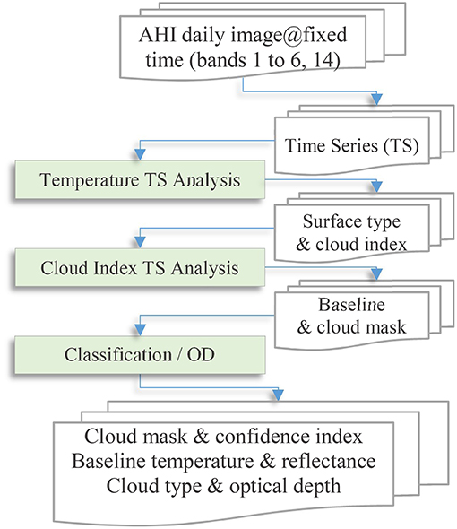
Figure 1. Work-flow for cloud masking based on time-series (TS) analyses, and cloud classification and optical depth (OD) retrieval using radiative transfer modeling.

Cloud Masking

The first step of the algorithm (Figure 1) is to sort the Himawari bands into time series with fixed acquisition time from multiple dates. For example, the daily images acquired at 02:00 UTC were collected into one time series per pixel. This choice for the time series, instead of all consecutive 10-min images throughout the day, is based on the following considerations: (i) it is rare for surface pixels to experience, over consecutive days but at fixed times, substantial changes compared to that induced by overlaying clouds; and (ii) a daily time series of all consecutive observations will include daily cycles of reflectance and temperature due to daily sun elevation and modulations by surface properties such as thermal inertia and soil moisture. These daily cycles would have to be modeled to an accuracy level higher than the minimum of distinguishable signals caused by overlaying cloud layers. This is very challenging, and any modeling error will have a direct impact on the sensitivity of cloud detection, as discussed below. Another factor that affects the apparent surface reflectance is the solar position. Its change, however, is very slow as the time series is built at fixed daily acquisition time. All such slow variations, including other natural variations such as that caused by plant phenology, form a slow changing baseline reflectance against which rapid changes due to the onset of clouds are detected. Therefore, such slow variations would not affect the ability of the algorithm on cloud detection. The length of time series is also not critical, the only consideration is: “are there sufficient number of clear days from which the baseline reflectance can be extracted?” Details on baseline reflectance and cloud detection are discussed below.

The presence of clouds in a pixel generally increases its top of atmosphere (TOA) reflectance, especially in the visible bands, but decreases its apparent temperature due to the higher altitude of clouds. Both factors can be used for cloud detection. Here a cloud index, denoted I_c, was defined to combine the two factors to maximize the difference between cloudy and clear (cloud-free) pixels:

$\begin{array}{ll}{I}_c=\frac{T_{max}-T}{T_{scl}}{R}_b& (1)\end{array}$

where T (in K) is the brightness temperature of band 14 (11.24 μm), and R_b is the reflectance of either band 2 (0.51 μm) or band 6 (2.3 μm) depending on the surface type (discussed below). T_max = 373.15 K and T_scl = 100 K have been chosen to balance the relative sensitivity of temperature and reflectance. This cloud index is modified from Qin et al. (2015) where T appeared in the denominator as I_c = R_b/(T − T_min). The advantage of this modification is that the sensitivity of I_c to change of T, ∂I_c/∂T = −R_b/T_scl, does not depend on the absolute value of temperature (T) and therefore is equally sensitive over latitudes with different surface and cloud top temperatures. While this index is only tested in this study over the Australia region, the chosen T_max is large enough to cover any part of the world and therefore Equation (1) should be applicable worldwide.

The choice of the spectral band for R_b in Equation (1) depends on the surface type in the pixel. For the Australian continent the majority of surfaces (semi-desert, rangeland, agriculture, and forest) have low blue/green band reflectance, providing a striking contrast to clouds which always have high reflectance in these bands. Such surfaces are referred to as “type-1 surfaces” herein. For type-1 surfaces, AHI band 2 (0.51 μm) was the reflectance component in the cloud index. Due to Rayleigh scattering, band 1 (0.47 μm) often has a higher TOA reflectance during clear conditions, and so is less sensitive compared to band 2, especially when the sun is low and/or for areas with a large viewing zenith angles near the edge of the imaged disk. Water bodies—both in-land and oceans—also have low surface reflectance in the blue/green bands, and so were treated the same as type-1. In addition to type-1, there is a very small fraction of the Australian continent that has high reflectance in the blue/green bands, such as salt lakes and snow regions. For these surfaces, hereafter denoted “type-2,” band 6 (2.3 μm) was the reflectance component in the cloud index because it is normally relatively lower than clouds. Examples of typical surface and cloud reflectance spectra are presented in section Qualitative Assessment.

For the majority of the Australian continent the surface type classification remains invariant over months to years, but temporal changes do occur in areas such as salt lakes or areas subject to intermittent flooding or snow. To deal with the different, and in some parts, changing surface types, the surface type needs to be determined at given location and times. This is accomplished using an initial time-series filtering on temperature only, which removes likely cloudy time points, followed by a classification on cleared data points to determine the surface type at any time. Compared to reflectance, surface temperature experiences more rapid but smaller fluctuations, especially over land, and so it is less sensitive on its own for detection of weaker (thin or partial) clouds. On the other hand, surface temperature rarely undergoes dramatic changes over a short time (days) even when the surface is changing from one type to another. Temperature therefore is a noisy but reliable predictor for surface type classification.

Filtering, for both cloud index and temperature-only time series, was implemented iteratively, where each iteration was conducted using the Lee (1986) algorithm. Figure 2 illustrates this process for a case of the cloud index, where in the first iteration all data points are fed to the Lee filter, and the filtering output is shown as a red line. Points that are above the red line plus a small margin, shown as red circles, are masked as cloudy and are subsequently removed from further iterations. This is repeated until no more data points can be removed. The small margin mentioned above, denoted as ΔI_c,min, is the only threshold value used in this algorithm, which will be discussed in more details later in the context of confidence level calculation. For the case shown in Figure 2, which is a relatively simple case and used here for clarity, only three iterations were required. For temperature filtering, the only difference is that data points that are lower than the Lee filtering output minus a margin are masked as cloudy and removed from further iterations.

FIGURE 2

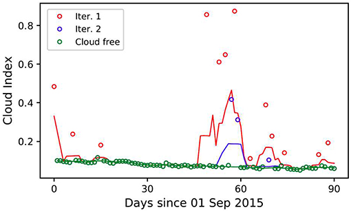
Figure 2. Iterative filtering process for cloud masking. In this case three iterations were required to remove all the cloudy points. The lines are the output of Lee filtering after each iteration, and the circles indicate the points being removed at each iteration. Shown here is the case of cloud index filtering for a 3-month period and 02:00 UTC. On the figure “Iter.” denotes Iteration.

After removing likely cloudy time points based on the initial filtering of the temperature time series, pixels (at cloud-free time points) are classified as type-2 if either of the following two criteria is satisfied: (i) R₂ > 1.5R₆ and R₂ > 0.25; or (ii) R₂ > 0.35. All remaining pixels are type-1. For pixels where surface type does change, the surface type at cloudy time points is assigned using nearest cloud-free points. This simple classification of surface type was designed for the Australian continent and its surrounding waters, where the continent experiences minimal land-use change (Donohue et al., 2009). For other parts of the world modification may be required. However, the time-series-based cloud detection approach presented here is robust and tolerable to some misclassification of the surface type.

Cloud Masking Confidence

After removing all the cloudy time points, the cloud index, I_c, is interpolated to all cloudy time points to form a baseline cloud index, denoted as I_c,base, and the difference between I_c and the baseline is denoted as ΔI_c = I_c − I_c,base. As discussed above, if a time point has a I_c greater than I_c,base by a margin of ΔI_c,min, i.e., ΔI_c ≥ ΔI_c,min, the time point is classified as cloudy. Otherwise the point is classified as clear. The line defined by I_c,base + ΔI_c,min therefore is a line that separates cloudy time points from clear points. The higher the I_c of a point is above the separation line the more likely the point is cloudy. Similarly, the lower the I_c is below the separation line the more likely the point is clear. The position of I_c relative to the separation line, therefore, can be used to define a two-way confidence level as discussed below.

Firstly a relative cloud index, i_c, is defined as the relative difference between I_c and the separation line as:

$i_c=\{\begin{array}{c}\frac{\Delta I_c-\Delta I_{c,min}}{\Delta I_{c,min}}\text{ cloudy}:\Delta I_c\ge \Delta I_{c,min}\\ \frac{\Delta I_{c,min}-\Delta I_c}{\Delta I_{c,min}}\text{ clear}:\Delta I_c<\Delta I_{c,min}& (2)\end{array}$

Secondly, the relative cloud index, i_c, is logarithmically transformed to calculate the confidence level, c, for all (cloudy and clear) time points as:

$\begin{array}{ll}c=min(\lfloor c_f\rfloor ,C),c_f=\frac{log(\sigma i_c+1)}{log(\sigma I+1)}(C+1)& (3)\end{array}$

where $\lfloor c_f\rfloor$ is the floor function that returns the integer part of c_f, and min(x, y) clips the confidence level to the maximum value C. We used ΔI_c,min = 0.015, C = 15, σ = 1 and I = 3 for cloudy cases or I = 2 for clear cases. The confidence level, therefore, is from 0 to 15.

When i_c = 0, i.e., the cloud index is exactly on the separation line, the confidence level will be zero. Through the logarithm function, confidence levels are allocated nonlinearly to different range of i_c favoring the lower range of i_c, and the allocation is controlled by σ in Equation (3). Increasing σ will distribute more confidence levels to the lower range of i_c, and vice versa. Figure 3 shows the confidence function as function of i_c. For cloudy cases, exactly half of the available confidence levels (0–15) are allocated to i_c in the range i_c < 1.0, and the other half are allocated to i_c ≥ 1.0 until the confidence level reaches the maximum at i_c = I = 3 when the confidence level is clipped to the maximum. By allocating more confidence levels to the lower range of i_c, better granulation is provided in the post-processing reclassification (discussed below) without excessively increasing the amount of storage required.

FIGURE 3

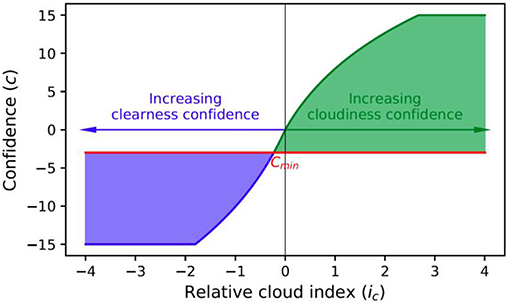
Figure 3. Confidence, c, as function of relative cloud index, i_c, for parameters of present work (C = 15, σ = 1 and I = 3 for cloudy cases or I = 2 for clear cases). Note that for the clear case (in blue) the negative of confidence and relative cloud index are plotted to show the two-way nature of the confidence level. The shaded areas illustrate re-classification using a confidence threshold, c_min = −3 in this plot, which reclassifies some originally clear pixels as cloudy resulting in the reclassified clear pixels with higher clearness confidence.

The two-way confidence level allows for post-processing reclassification, as illustrated in Figure 3, using a confidence threshold, c_min, shown as the red line. In the figure the shaded blue and green areas indicate the reclassification results, and for the purpose of illustration the negatives of i_c and c are shown for the case of clear pixels. In the case of Figure 3, by moving c_min below zero some of the originally clear pixels are reclassified as cloudy leaving the remaining clear pixels with a higher overall clearness confidence but at the expense of the overall cloudiness confidence. The opposite effect can be achieved by moving c_min above zero.

Cloud Classification and Optical Depth Retrieval

A cloud classification and optical depth retrieval algorithm has been developed, based on radiative transfer modeling and utilizes the cloud masking results described previously. The cloud masking process detects clouds and also aerosols when the aerosol layer is substantial (with optical depth greater than 0.5) and becomes opaque such as in smoke plumes or dust storms. Hereafter, the term “clouds” also refers to opaque levels of aerosol layers.

Similar to the cloud index baseline discussed above, a TOA reflectance baseline and a TOA temperature baseline can also be generated. As any substantial aerosol layers are also detected and masked in the above detection process, the remaining baselines may only contain background aerosols which, for Australian, is stable with low optical depth in the range of 0.02–0.05 (Mitchell et al., 2017). By assuming a constant background aerosol optical depth, the type and optical depth of “clouds” can be determined by radiative transfer modeling in the following two steps.

1) Using the assumed background aerosol optical depth, which is zero in current implementation for simplicity considered the very low level of background aerosols, the spectral reflectance at the surface can be determined from the baseline TOA reflectance using an inverse radiative transfer. As we are dealing with “clouds” (meaning clouds and opaque aerosols as defined previously) with substantial optical depth, the surface contribution to TOA reflectance decreases rapidly with increasing optical depth, and bi-directional reflectance distribution function (BRDF) of the surface becomes a less critical factor. For simplicity the Lambertian approximation was assumed and the TOA reflectance is related to surface albedo, ρ, as (Liou, 1980; Qin et al., 2015):

$\begin{array}{ll}{R}_{toa}(\tau ,{\mu }_0,{\mu }_v,\varphi )=R_a(\tau ,{\mu }_0,{\mu }_v,\varphi )+\frac{\rho T_s({\mu }_0)T_a({\mu }_v)}{1-\rho \overline{r}}& (4)\end{array}$

where R_a represents the reflection by the atmosphere, and the second term represents the interactions between the atmosphere and the surface. T_s and T_a are transmittance functions accounting the attenuation due to the atmosphere, $\overline{r}$ represents the global reflection by atmosphere at the surface, τ is the total optical depth (at 0.55 μm) of the atmosphere including the absorption and scattering of molecules and “clouds,” and μ₀, μ_v and ϕ are, respectively, cosine of solar zenith angle, cosine of view zenith angle, and relative azimuth angle between the sun and the satellite. The time series of surface albedo, derived from the baseline TOA reflectance using Equation (4), is referred to as the baseline surface albedo.

2) With the baseline surface albedo now available, the TOA reflectance can be computed using Equation (4) given the aerosol/cloud optical parameters. The per-pixel type of “clouds” and optical depth were determined by testing a set of predefined “cloud” models (i.e., predefined single scattering albedo, phase function and extinction coefficient spectral profile) and by minimizing the following error function:

$\begin{array}{ll}{f}_{err}=\frac{(f_{err}^{(1)}+w{f}_{err}^{(2)})}{(1+w)},w=0.1*\overline{R}& (5)\end{array}$

$\begin{array}{ll}{f}_{err}^{(1)}=\frac{1}{5}{\displaystyle \sum _{b=1}^5}|{R_b-R}_b^m(\tau )|& (6)\end{array}$

$\begin{array}{ll}{f}_{err}^{(2)}=\frac{1}{10}{\displaystyle \sum _{b_1=1}^4}{\displaystyle \sum _{b_2=b_1+1}^5}|\frac{R_{b_1}}{R_{b_2}}-\frac{R_{b_1}^m(\tau )}{R_{b_2}^m(\tau )}|& (7)\end{array}$

where R_b is the TOA reflectance of band b, $R_b^m(\tau )$ is the reflectance of band b at optical depth τ computed using Equation (4), R is the mean TOA reflectance. The first part of the error function, denoted by the superscript (1) in Equation (5) and defined in Equation (6), is the mean absolute difference of modeled and measured TOA reflectance, and the second part of the error function, denoted by the superscript (2) in Equation (5) and defined in Equation (7), represents the spectral resemblance between model and data. In this work, AHI bands 1–5 were used. While band 6 (2.26μm) is involved in cloud detection, we found that the model predicted AHI band 6 cloud top reflectance is usually lower than measurements, especially for the water clouds (cumulus and stratus), and therefore band 6 is not used in the classification. The reason of the poor model performance at band 6 is to be investigated.

Lookup tables (LUT) were employed for operational radiative transfer calculations. R_a, T_s, T_a, and $\overline{r}$ in Equation (4) were pre-computed and stored in LUT's for a sufficiently wide range of solar and view angles and optical depth from 0 to 100, for each of the aerosol and cloud types (see Table 1 and further discussion shortly). The Vector Green's function and Discrete-Ordinate-Method (VGDOM) radiative transfer code (Qin and Box, 2005, 2006) was used to solve the plane parallel radiative transfer equation. This code contains an implementation of the Discrete-Ordinate-Method with delta-M scaling (Nakajima and Tanaka, 1986) to handle large cloud particles causing very strong forward scattering. Because of the delta-M scaling the maximum number of streams is limited to 64, otherwise the exact number depends on the number of terms required to expand the phase function.

TABLE 1

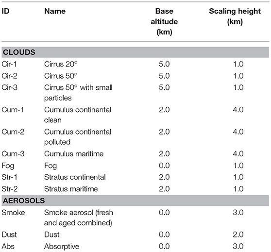
Table 1. Optical models used in “cloud” classification.

The cloud optical models used herein were the OPAC (Optical Properties of Aerosols and Clouds) models (Hess et al., 1998), while the aerosol models are from (Qin and Mitchell, 2009). For all clouds and aerosols, a single layer is assumed currently, with the optical depth vertical profile assumed to follow the exponential rule, i.e., the optical depth τ(h) = τ₀(h₀)exp[−(h − h₀)/H], where H is the scaling height and τ₀ is the optical depth at the base of the layer, h₀. The cloud and aerosol models, their base altitude and scaling height used in this work are listed in Table 1. For simplicity, the US-1962 standard atmosphere model was used to describe the molecular atmosphere. The optical depth due to molecular atmosphere is extracted from the 6S code (Vermote et al., 1997) in this work, but it can also readily be evaluated using, for example, MODTRAN (Berk et al., 2014).

As the Australian continent is relatively flat, surface elevation is assumed to be constant at mean sea surface level in the current implementation, but refinement may be required in future work. Subpixel cloud fraction is not considered, therefore the retrieved “cloud” type and optical depth represent a radiative mean of the whole pixel. Due to the assumed constant background aerosols, the baseline surface albedo may be affected. However, because the background aerosol loading is small (Mitchell et al., 2017), the effect on optical depth retrieval will also be small–on the same level as the background AOD, i.e., 0.02 to 0.05.

Results and Discussion

Cloud Masking Validation

Figure 4 presents a typical example of cloud masking and the associated confidence calculation. The upper row shows significant amount of clouds across the continent. For areas with continuous clouds, clouds are masked with high confidence. The confidence however decreases as expected toward the edges of clouds or in partly-cloud pixels (i.e., mixed pixels where cloud does not cover the entire pixel), when clouds become less distinguishable from clear surface. The lower row in Figure 4 shows a small region of the continent, indicated by the black rectangle in the upper row, showing broken clouds scattered through the area. These broken clouds are masked correctly although their confidence varies.

FIGURE 4

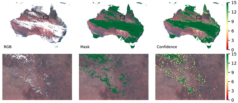
Figure 4. Example of RGB composition, cloud mask and confidence for an AHI image acquired at 02:00 (UTC) on 2nd May 2016. The upper row shows continuous clouds across the Australian continent, and the lower row shows the details for a small region marked in the upper row with black rectangles. The left column shows the RGB image in which Red is AHI band 3 (0.64 μm); Green is band 2 (0.51 μm) and Blue is band 1 (0.47 μm). The central column shows the cloud mask (binary with cloud colored dark green), and the right column illustrates the cloud confidence (0–15) score. All the cloud mask and cloud confidence images are overlaid on the same RGB image as shown in the left column.

An quantitative validation using the Cloud-Aerosol Lidar with Orthogonal Polarization (CALIOP) instrument (Winker et al., 2009) was conducted. As a dedicated sensor for cloud and aerosol detection and profiling, and with its altitude resolving ability, this instrument is particularly sensitive to the presence of “clouds” without interference of the surface, and therefore provides a reliable reference against which cloud masking products from other sensors can be validated (Wang et al., 2016; Karlsson and Hakansson, 2018). Figure 5 shows the hit rate, defined as the proportion of pixels identified by both AHI and CALIOP as either clear or “cloudy,” as a function of confidence threshold, c_min(discussed above and in Figure 3). Shown also in Figure 5 are the miss rate and its components: AHI clear–CALIOP cloudy (clear-cloudy), AHI cloudy–CALIOP clear (cloudy-clear). Figure 5 shows that at c_min = −3 the clear-cloudy and cloudy-clear rates reach an equality. This indicates that the current cloud mask threshold, ΔI_c,min in Eq (2), is too high that some cloudy pixels are misclassified as clear. Such misclassifications can be corrected by using the confidence threshold, c_min. At the neutral point, c_min = −3, the overall hit rate reached its maximum of 0.872, while the overall miss rate reached its minimum of 0.128. This suggests that this neutral point is also the optimum c_min confidence threshold.

FIGURE 5

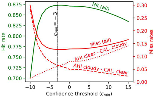
Figure 5. AHI-CALIOP cloud mask hit rate (in green) and miss rates (in red) as functions of confidence threshold (c_min, see text). At the neutral point, c_min = −3, the clear-cloudy and cloudy-clear rates reach equality while the hit rate reaches its maximum and miss rate reaches its minimum. Data was collected over both land and water for the region (110°E, 155°E, 10°S, 45°S) from 6th Jul 2015 to 30th Jun 2016.

The hit rate of 87.2% is slightly better than (Stubenrauch et al., 2017) where the cloud detection from Atmospheric Infrared Sounder (AIRS), also an altitude resolving sensor, is compared with CALIOP and hit rates of 85% over ocean and 82% over land were reported. Wang et al. (2016) reported a hit rate of 77.8% for the MODIS MYD06 cloud product when validated against the CloudSat-CALIOP combined retrieval. The hit rate of 87.2%, however, is much lower than we expected from the visual assessments we performed. This discrepancy is caused by the small footprint of the CALIOP sensor, which has a ground beam size of 70 meters and takes measurements every 330 m along the ground track (Winker et al., 2009). Comparatively, the AHI data used here has 2 km resolution and when the AHI pixel is partially clouded, the CALIOP laser beam may or may not hit any clouds within the matchup AHI pixel resulting in an uncertainty which depends on the cloud fraction. If the CALIOP beam size is zero and the CALIOP shots only once within the matchup AHI pixels, the uncertainty would reach the maximum when the cloud fraction is at 50%, when the pixel is most fractured by area. However, because of CALIOP's beam size and it takes measurements ~6 times within each matchup AHI pixel, the actual cloud fraction at which the uncertainty maximizes will be less than 50%. Noting that a matchup AHI pixel is reported as cloudy by CALIOP if any one of the 6 shots hits—even just partially—the cloudy area within the AHI pixel.

The effect of footprint difference is quantified using a regional cloud fraction, the proportion of cloudy pixels within a window of ±30 CALIOP pixels (or ±30 km), calculated from the CALIOP data set. Using this regional cloud fraction as a proxy for AHI pixel level cloud fraction, Figure 6 shows that, when the region is either totally clear or overcast, the two instruments agree with each other at a very high average ratio of ~0.98. However, the agreement dramatically deteriorates once the region becomes partially cloudy, with the hit rate reaching the minimum at ~40% cloud fraction. The inset table in Figure 6 further groups the overcast pixels (i.e., ≥0.95 cloud fraction) by optical depth. It shows that the hit rate remains high regardless of the optical depth. This indicates that, once footprint difference is accounted for, the hit rate is very high even in the case of thin clouds with optical depth less than 0.25, which is about the lower limit of detectable optical depth of 0.225 suggested by Karlsson and Hakansson (2018) or 0.3 by Sun et al. (2014). We also note that, among the ~52 million matchup points, more than half (56.2%) of them are in the total clear or overcast bins (i.e., < 5% or > 95% cloud fraction), and the remainders spread quite evenly into the other 18 bins (2.4% mean, 2.1% minimum and 3.5% maximum). Hutchison et al. (2014) validated the VIIRS cloud mask (VCM) product against CALIOP and also showed the impact of cloud fraction on hit rate. They showed when only pixels with high confidence (an index converted from cloud fraction) are included, a hit rate of ~95% was reported, though Hutchison et al. (2014) also excluded pixels with optical depth less than 1.0.

FIGURE 6

Figure 6. Hit and miss rates as functions of cloud fraction (see text), showing that the hit rate is very high when the sky is either totally clear or overcast but the hit rate decreases rapidly when the sky becomes fractured. The inset table groups pixels with cloud fraction >0.95 by optical depth, showing that when the factor of cloud fraction is excluded, the hit rate remains close to unity even for thin clouds with optical depth less than 0.25. Data was collected over both land and water for the region (110°E, 155°E, 10°S, 45°S) from 6th Jul 2015 to 30th Jun 2016.

In addition to footprint, geolocation difference could also impact the hit rate. This is examined in Figure 7 where the CALIOP tracks were firstly displaced by up to an equivalent of 1.5 AHI pixels (3000 m) in steps of 0.1 AHI pixels before they are matched with AHI. Figure 7 shows that there is a geolocation difference of about 1414 m, but this difference does not impact the hit rate substantially. When the region is totally clear or totally overcast (i.e., not partially cloudy), small geolocation differences does not cause much variation in the hit rate, but when it is partially cloudy, the footprint factor discussed above is so dominating that the geolocation difference becomes almost irrelevant. The time difference between the two sensors, which is less than 5 min, is expected to have only minor effect on the hit rate and therefore is not examined here.

FIGURE 7

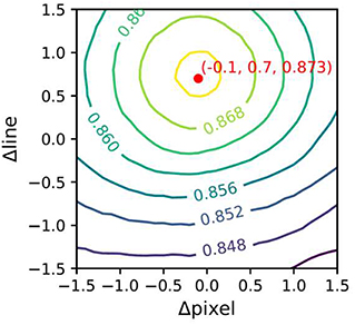
Figure 7. AHI-CALIOP cloud mask hit rate as function of pixel and line displacement (in AHI pixels, see text), indicating a geolocation differences between AHI and CALIOP of−0.1 AHI pixels (~200 m) and 0.7 AHI lines (~1,400 m), or a direct line difference of 1,414 m. These are shown in red and the third value in that array is the maximum cloud hit rate. Hit rate is calculated for all conditions (total clear to overcast) over land and water for the region (110°E, 155°E, 10°S, 45°S) from 6th Jul 2015 to 30th Jun 2016.

Classification and Optical Depth Retrieval

In this section, a general discussion and qualitative assessment of the classification will be provided first, followed by an indirect quantitative validation against in-situ measurements of solar flux. Further, geographical distribution of cloud fraction is compared with ISCCP climatology, and the geographical distributions of optical depth are presented lastly in the section.

Qualitative Assessment

Examples of cloud classification and optical depth retrieval are provided in Figure 8, for the Australia region. Figures 8a,b show a low pressure system dominating the eastern half of the continent, and a trough is located off the south coast. From the clouds accompanying these systems, two sub-regions are selected and their details are presented below.

FIGURE 8

Figure 8. Example cloud classification and optical depth retrieval results, obtained at 00:00UTC on 31 Dec 2015. (a) Is RGB composite for the whole Australian region with AHI band 3 (0.64 μm, red), band 2 (0.51 μm, green) and band 1 (0.47 μm, red). The two rectangles, labeled R1 and R2 respectively, mark two sub-regions that are examined in detail below. (b) Shows the mean sea level pressure (MSLP) analysis at 00:00 UTC (source: Australia Bureau of Meteorology). (c–f) Are, respectively, the RGB composite, cloud classification, cloud-top-temperature and optical depth for sub-region R1. (g–j) respectively provide the same information as (c–f), except for sub-region R2.

For sub-region R1, the RGB composite (Figure 8c) shows that clouds in the region are convective with individual cells clearly identifiable. This is confirmed by Figure 8d which shows that most clouds in the region are classified as cumulative. The size of cloud cells in the lower-left part is much larger with some of the cells classified as stratiform clouds. An examination of the time series showed that increasingly more of the large cells were classified as stratiform clouds, suggesting that some cells were probably experiencing transition from altocumulus to stratocumulus. Figure 8e shows that the cloud top temperature in the lower-left part is slightly lower, probably due to stronger convection in the lower-left part leading to more diverse cloud droplets. As a result some originally cumulative cells (with narrower size spectrum) are classified as stratiform with wider size spectrum (Hess et al., 1998). Due to the critical effects of subtropical marine stratocumulus on Earth's energy balance (Wood, 2012; Yuter et al., 2018), satellite data, such as shown in sub-region R1, will play an important role in the still intensive researches in understanding their formation and dynamics.

Sub-region R2 is separated into two parts, defined by the southern coastline (Figure 8f). The wispy cloud texture of the upper-right part of Figure 8g clearly suggests that the cloud should be cirrus, which is confirmed by classification (Figure 8h). The cloud top temperature of these clouds are low at ~240 K (Figure 8i), about 70 K lower than the surface, meaning that the clouds must be high clouds and supporting the classification. The lower-left part of sub-region R2 consists mostly uniform clouds as shown in Figure 8g, which were classified mostly as stratiform and cumulative clouds Figure 8h. Compared to the surface, the cloud top temperature is about 30 K lower (Figure 8i), suggesting the clouds should be middle to low clouds. This is consistent with the classification.

In Figure 9 we examine detailed examples of cloud detection and cloud classification over different surface types with different cloud types. The four locations represent a range of surface types: (i) forest; (ii) rangeland; (iii) snow; and (iv) ocean. Among the locations, three (i.e., forest, rangeland and ocean) are of type-1 and one is of type-2 (i.e., snow; see section Method for more type-1/type-2 details). For each location, three time-points are selected corresponding to the broad cloud types, cirrus (blue), cumulus (green) and stratus (red). Figure 9 illustrates the method of cloud detection, the sensitivity on detecting especially thin and partial clouds. This is demonstrated by both cloud index time series (left column) and the separation of TOA reflectance from clear day reflectance (right column). Detecting clouds over type-2 surface is more challenging than other surface types as shown in the case of snow (third row). The TOA reflectance (circles) is hardly distinguishable from the baseline clear day reflectance (squares) in the first 4 bands. However, by combining temperature and band 6 reflectance in the type-2 cloud index, clouds become clearly distinguishable from the baseline. The third row also shows a case when the surface changes its type, from type-2 (days < 20) to type-1 (days > 40), during snowmelt the band 2 reflectance dropped from ~0.8 to ~0.1. Figure 9 (right column) shows that the radiative transfer model generally predict the TOA reflectance very well with closely matching TOA reflectance, regardless of the optical thickness and type of the clouds.

FIGURE 9

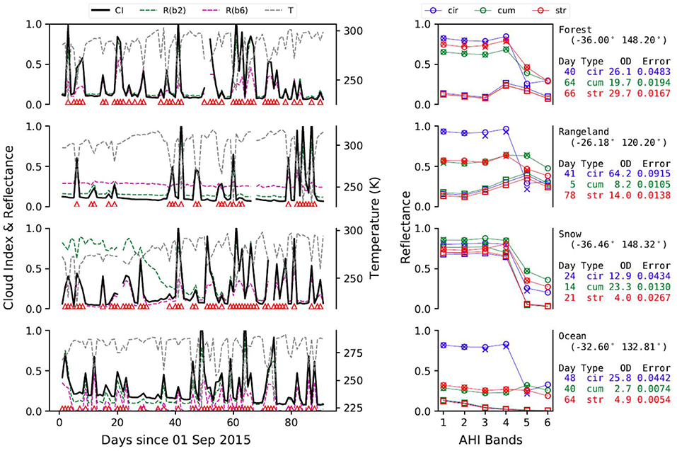
Figure 9. Examples of cloud detection and cloud classification for various surface types (from top to bottom) and several cloud types. The left column shows results of time-series analysis for the detection of clouds, illustrating the sensitivity of the analysis on detection of thin or partial clouds. Detected cloudy time points are marked by red triangles along the x-axis. AHI TOA reflectance (b2 and b6) and temperature are shown along with cloud index. The right column shows cloud classification by radiative transfer modeling of AHI TOA reflectance, on 3 days when different types of clouds (shown in three colors) are present. Blue denotes cirrus clouds, green cumulus and red stratus clouds. The “Day” refers to the day since 1 September 2015. The squares are the baseline (clear day) TOA reflectance, circles are TOA reflectance, and crosses are modeled TOA reflectance.

Further information on modeling error is provided in Figure 10, which shows mean modeling error Figure 10a and the maximum error at 95th percentile (derived as mean error plus 2 standard deviation; Figure 10b). Figure 10b shows that the maximum modeling error is mostly less than ~0.06 over the entire Australian region, indicating good agreement between model and data (see Figure 9 right column). The ability to model the cloud top spectral reflectance confirms that the OPAC cloud models provided adequate description of the cloud optical properties, and that the radiative transfer scheme used in this work is suitable in terms of radiative consistency. However, high maximum modeling error over the ephemeral salt lakes in central Australia (the small red area in Figure 10b) is because parts of these salt lakes can change their reflectance within a day, when rainfall turned salt surfaces into specular reflectors, reflecting the light away from the satellite and lowering the measured reflectance instantly. Other changes also occur in these salt lakes such as lateral inflowing standing water causing the salt crust to dissolve or being covered by standing water which carries high sediment loads, though these process take longer time scales (Mernagh, 2013).

FIGURE 10

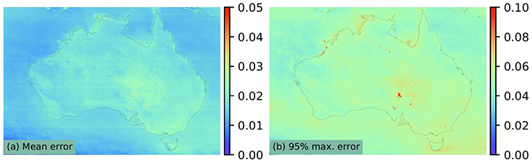
Figure 10. Error characterization of the Australian region from 6 Jun 2015 to 30 Jun 2018 for daylight hours (i.e., 22UTC to 8UTC or 8–18 Australian east standard time). Part (a) is the mean model error, defined by Equation (5), and (b) maximum error at the 95th percentile.

In addition to clouds, thick aerosol layers are also detected and classified, as part of the “cloud” detection and classification. Figure 11 shows an example of smoke plume detected in North Territory, Australia. Fine particles such as those originating from bush fires and hazard reduction burns have a range of impacts on human health including premature mortalities (Dennekamp et al., 2015; Haikerwal et al., 2015; O'Keeffe et al., 2016; Horsley et al., 2018). Smoke plumes quantified from this work could be useful in health impact analysis. Savanna biomass burning, as shown in Figure 11, contributes substantial amount of carbon emission (Hurst et al., 1994). Globally landscape and biomass fires contributes 2–4 Pg C year⁻¹ CO₂ emission (Bowman et al., 2009), or 20–40% the amount of carbon as that emitted from fossil-fuel combustion (Beringer et al., 2015). The method developed here therefore provides a potential approach to account carbon emissions from bush fires.

FIGURE 11

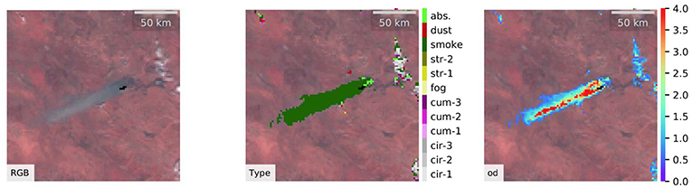
Figure 11. Detected smoke over the northern Australian continent at (134°E, 20°S) at 02:00 UTC on 10th Nov 2015.

Validation by Surface-Level Solar Flux

While very challenging to quantitatively validate the cloud class and optical depth directly, the downward flux at the surface can be calculated, using the retrieved cloud properties, and compared with in-situ measurements. This provides an indirect quantitative assessment of the quality of the retrieved cloud data. Three years (06 July 2015 to 30 June 2018) of solar flux data measured every 1 min at 11 sites across Australia (BoM, 2018) were collected and averaged to 10 min interval. Solar flux was also calculated using the retrieved cloud parameters at the 11 sites, each represented by the AHI pixel (2 km) nearest to the site. Both datasets were then matched up in time and matched records were averaged monthly. The bias and root mean square error (RMSE) of the calculated solar flux are shown in the “Original” columns in Table 2. Also shown in the table are the number of months of available measured data at each site, and the correlation coefficient. As a quality control we required the monthly data completeness to be greater than 90% for that month to be used.

TABLE 2

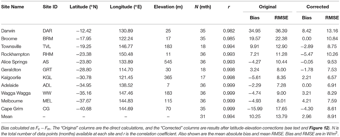
Table 2. Bias and RMSE of the AHI-based monthly mean solar flux (F_c) when compared to surface-level solar flux measurements (F_m).

It was noticed that the original bias shows a strong correlation with site latitude, as shown in Figure 12. While the cause of this systematic bias is still being investigated, the strong correlation provides the possibility to perform a correction to the calculated solar flux. It is also noticeable that the bias also depends on site elevation, which is expected (McVicar and Jupp, 1999) as currently a fixed surface elevation of the mean sea surface level is assumed, resulting in underestimation (negative bias) at high elevation sites due to the artificially extended atmosphere path. A regression of the original bias as function of latitude and elevation was performed, which gives bias = 43.5 + 1.3lat − 0.031elev with a mean regression error of 2.96 W/m². Using this relationship, the calculated flux was corrected by subtracting the above latitude-elevation related bias, and the new bias and RMSE of the corrected flux are listed in the “Corrected” columns in Table 2. Note that the correlation coefficient is not affected by this latitude-elevation correction.

FIGURE 12

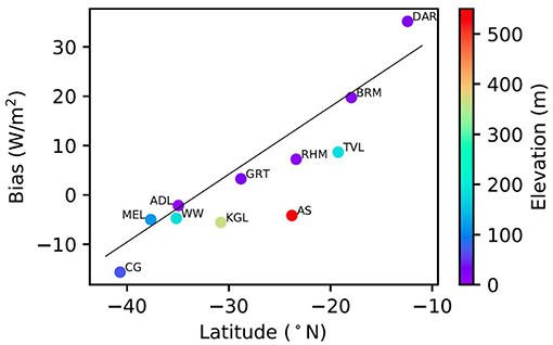
Figure 12. Dependence of the original flux bias on latitude and elevation, providing a way to correct the calculated flux. The points are labeled with site ID (Table 2) and the color of the circles indicates the elevation of the sites. The black line is the least square linear regression of the original bias after elevation correction (see text).

The new mean absolute bias and mean RMSE of the corrected flux are respecitvely 2.96 and 8.94 W/m². As a comparison, a mean difference (same as bias) of 2.017 W/m² and standard deviation (equivalent of RMSE) of 18.491 W/m² were reported by Zhang et al. (2004) for the solar flux data calculated using the ISCCP cloud products (Rossow and Schiffer, 1999). The results from our study are at least comparable to that of the ISCCP product, though we note that the ISCCP product is global. Our site specific bias and RMSE ressults are also similar to or better than the latitudinal zonal means reported by Zhang et al. (2004). The calculated vs. measured monthly mean solar flux at all sites are shown in Figure 13, for both before and after the latitude-elevation-correction. Figure 13a shows that the identified systematic bias exists across the whole flux range, i.e., in both clear and cloudy conditions, which indicates that cloud class and optical depth is not the source of the bias. Figure 13b shows significant improvements over the flux range, and the accuaracy of the monthly flux calculated from the derived cloud properties is high. In this sense, this analysis shows that the quality of current classification and optical depth retrieval should be at least comparable to that of the ISCCP products.

FIGURE 13

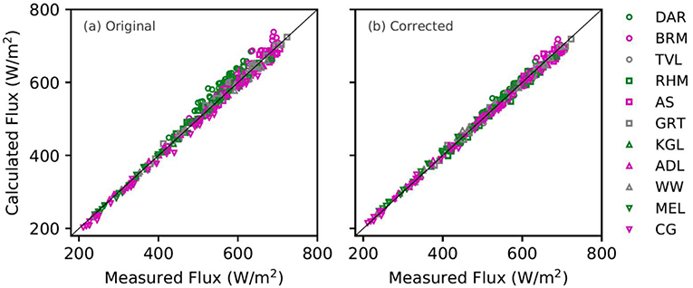
Figure 13. Comparison of measured monthly mean solar flux with that calculated from the retrieved cloud properties, before applying the latitude-elevation corrections (a) and after the corrections (b).

Regional Cloud Frequencies and Comparison With ISCCP

The geographic distribution of clouds is of great relevance to many areas such as climate and solar energy industry. Figure 14 shows, for Australia and part of Southeast Asia, the frequency of all clouds and the broad cloud types, seasonally and yearly. The statistics were derived from about two years of data from 1 Jan 2016 to 30 Nov 2017 for the daylight hours from 22UTC to 8UTC (8–18 Australian east standard time). Characteristically cloud coverage over the continent is lower than the surrounding ocean with the majority of the continent having an average cloud frequency of about 30% annually. Among the three broad cloud types (Table 1), cirriform clouds, the highest in altitude, have the highest overall frequency over the tropics while the stratiform clouds occurred most frequently to the south of the continent.

FIGURE 14

Figure 14. The left-most column (denoted column 1 here) shows cloud frequency for the all cloud types with columns 2–4 (from left to right) show the frequency of the broad cloud types. The austral seasons are provided in rows 1–4 and the yearly mean is given in row 5. Data obtained for the period from 1 Jan 2016 to 30 Nov 2017 for daylight hours from 22UTC to 8UTC (8–18 Australian east standard time).

Cirrus clouds, of ice crystals and high in altitude, are of particular interest to climate studies (Zhao et al., 2018). The seasonal and geographical distribution of cirrus clouds for the Australian region is shown in the second column in Figure 14. It shows that cirrus clouds are predominantly located in the tropics, which is consistent with previous studies. For example, Stubenrauch et al. (2017), Liao et al. (1995), Massie et al. (2002) and Wang et al. (1996) have all shown that high-altitude clouds dominate over tropical area while low-altitude clouds are relatively more enhanced over the mid-latitudes, particularly over the oceans to the west and south of the Australian continent. Sassen et al. (2009) showed the dominance of cirrus clouds over the tropical belt, with a whole-year mean frequency up to ~60%, which is comparable to Figure 14. Additional to the maximum frequency of tropical cirrus cloud, a secondary and much smaller local maximum is also visible over southern Australia around 45°S, which is consistent with Sassen et al. (2008) (Figure 2).

The cloud geographical distribution of Figure 14 was compared with the ISCCP mean cloud fraction (Figure 15), generated from the monthly climatology of ISCCP data (Rossow and Schiffer, 1999) from January 2010 to June 2015. Here the high clouds are cloud types 12–17 (cirrus, cirrostratus and deep convection), middle clouds are types 06–11 (altocumulus, altostratus and nimbostratus) and low clouds are types 00–05 (cumulus, stratocumulus and stratus). We note that all the above broad ISCCP cloud classes contain both ice and water clouds, while in current study ice clouds and water clouds are distinctively separated. Also, the ISCCP cloud amount represents the mean spatial cloud cover fraction within each cell of 1° × 1°, while Figure 14 shows the temporal frequency at each pixel (about 0.02° × 0.02°).

FIGURE 15

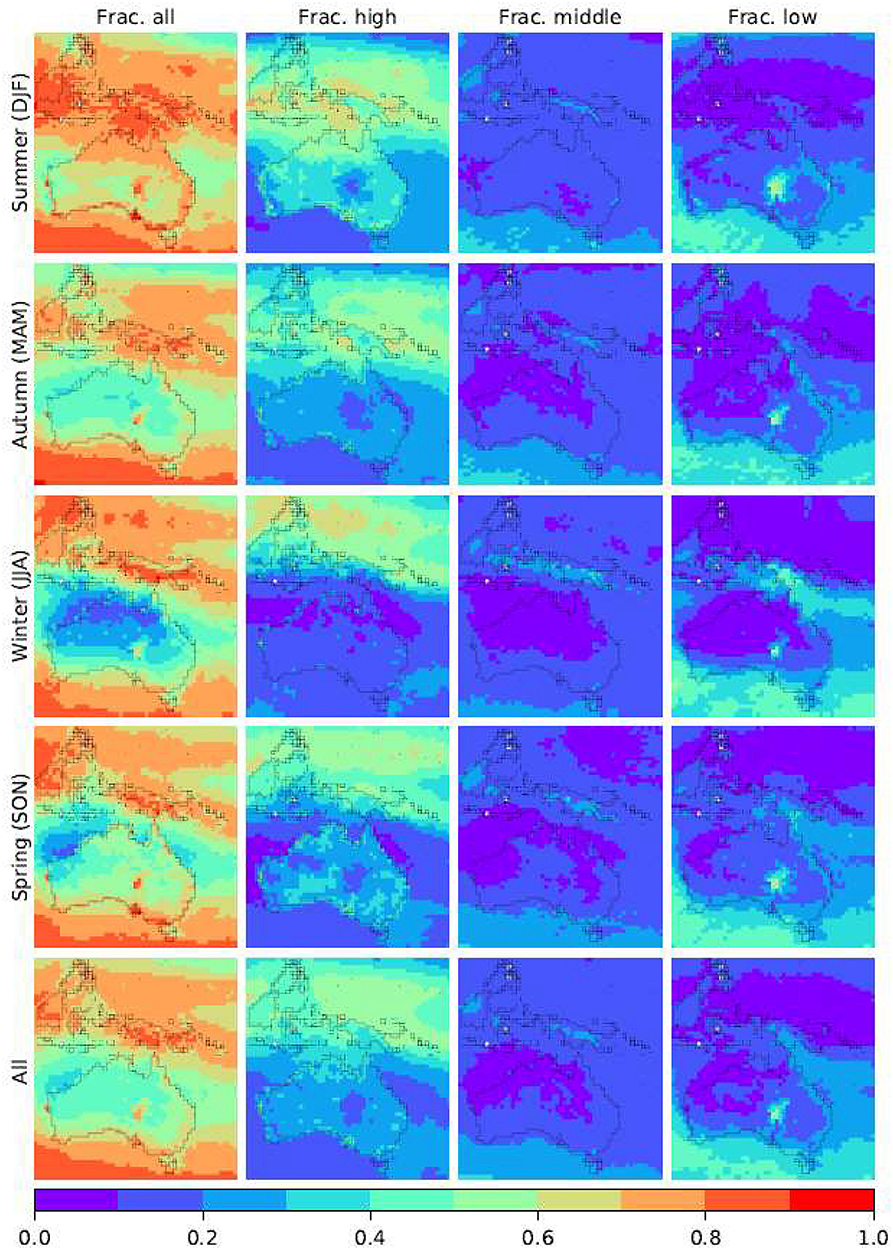
Figure 15. ISCCP climatology. The left-most column (denoted column 1 here) shows cloud frequency for the all cloud types with columns 2–4 (from left to right) show the frequency of the broad cloud types. The austral seasons are provided in rows 1–4 and the yearly mean is given in row 5. Data obtained for the period from Jan 2010 to Jun 2015 for daylight hours (00, 03, and 06 UTC).

Figures 14, 15 show that the two datasets resemble each other to a high degree, in both geographical pattern and magnitude, in the case of all-cloud-fraction (column 1 in both figures). For high clouds (ISCCP), or cirrus in present study, both datasets show high fractions in the tropics. They, however, differ from each other in the middle latitude zone where a clear minimum shown in present study is lacking in the ISCCP dataset. For the middle and low clouds (ISCCP), or cumulus and stratus (present study), the two datasets again highly resemble each other in broad geographical pattern. While the overall pattern and magnitude is very similar between the two datasets, it is noticeable that the relative fraction between the high clouds and low clouds is different. This is probably due to the difference in cloud categorization, and the optical properties of the cloud models may also differ from each other. For example, in present study the cirrus clouds represent all ice clouds, while in ISCCP the high clouds include both ice and water clouds.

In Figure 16 the seasonal and annual mean of cloud optical depth are presented. The optical depth of cirrus clouds is generally high which seems to contradict the usual understanding of cirrus which are thin and semi-transparent clouds which appears dark in satellite imagery. Indeed in the OPAC (Hess et al., 1998) model, the scope of cirrus is much wider than the name has suggested. It is used to represent all ice clouds including deep convection ice clouds which are often very thick and appears very bright. This is also shown in Figure 9 where it shows the cirrus reflectance can be as high as over 0.9 in the visible and near infrared bands. Another unexpected feature in Figure 16 is the relatively high stratus optical depth (last column) over the Lake Eyre Basin (located at southeast of central Australia), though the cloud frequency of the same area is low as shown in Figure 14. As the region is well known for being a major dust source region (Mitchell et al., 2017), this high optical depth may be an indication of misclassification by current algorithm. However, the optical depth peaks during winter and minimizes during summer is contradicting existing knowledge that the presence of dusts peaks in summer and minimizes in winter. It is therefore necessary to investigate further regarding the nature of the high stratus optical depth over the region. Further information about geographical distribution is presented in Figures 17, 18, where three lower optical depth thresholds are used to select the data for statistics. Again the high stratus optical depth over Lake Eyre is probably the most unexpected feature that should be investigated. We also note that the mean optical depth of stratus is generally lower than other two types, especially over the tropical area, despite its frequency is higher or comparable to the other two broad types.

FIGURE 16

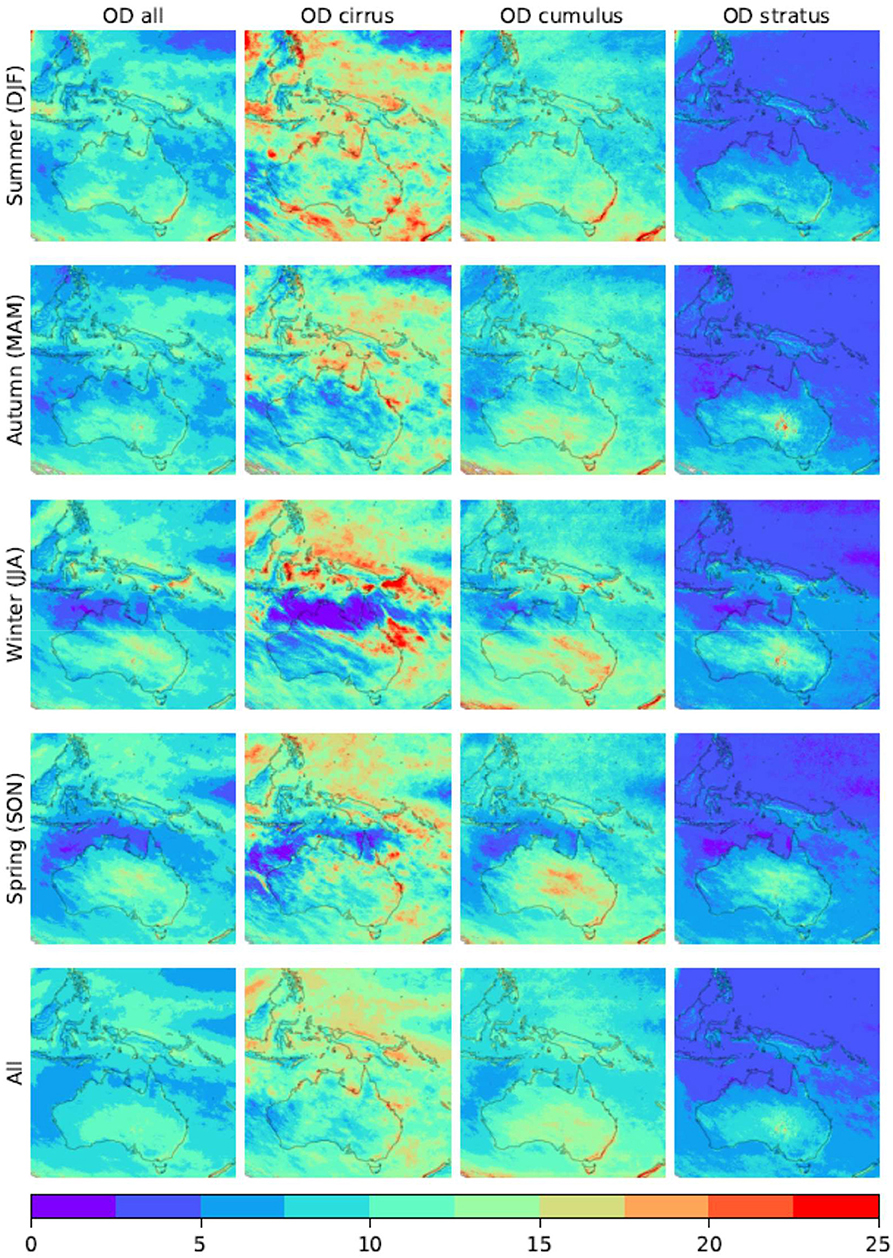
Figure 16. The left-most column (denoted column 1 here) shows cloud optical depth for the all cloud types with columns 2–4 (from left to right) show the optical depth of the broad cloud types. The austral seasons are provided in rows 1–4 and the yearly mean is given in row 5. Data obtained for the period from 1 Jan 2016 to 30 Nov 2017 for daylight hours from 22UTC to 8UTC (8–18 Australian east standard time).

FIGURE 17

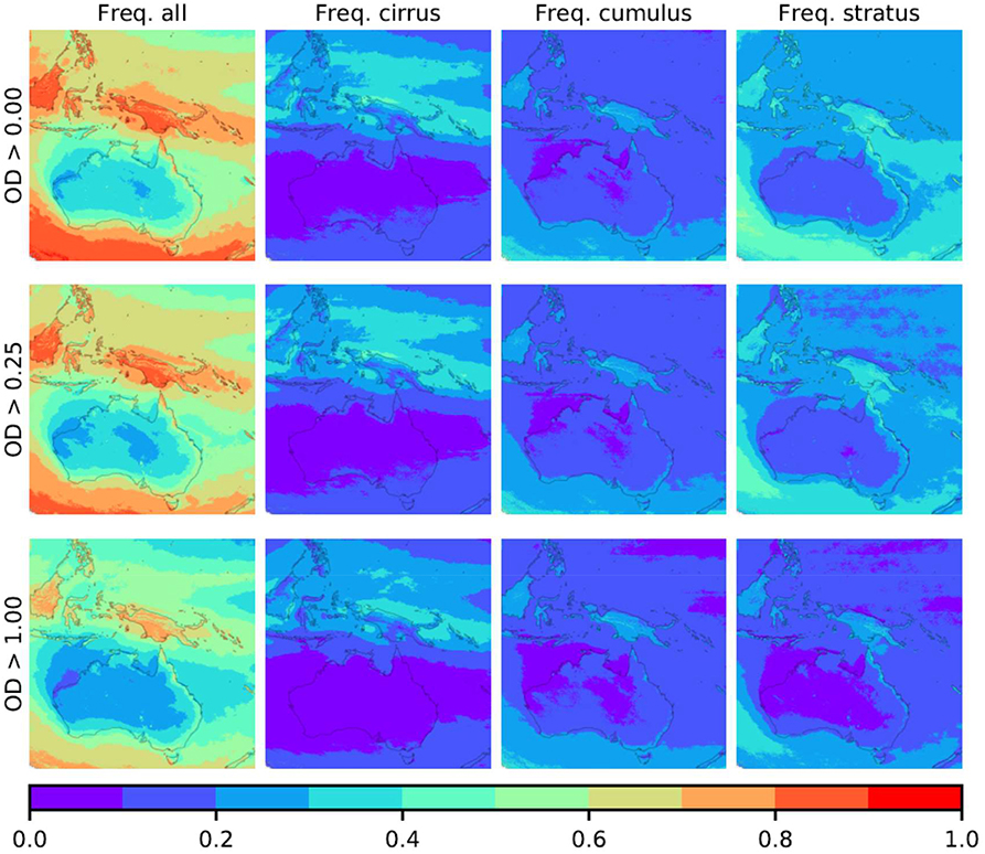
Figure 17. Change of yearly mean cloud frequency with lower optical depth (OD) thresholds: the top row shows all data; the middle row only when OD > 0.25; and the bottom row when OD > 1.0. Data obtained for the period from 1 Jan 2016 to 30 Nov 2017 for daylight hours from 22UTC to 8UTC (8–18 Australian east standard time).

FIGURE 18

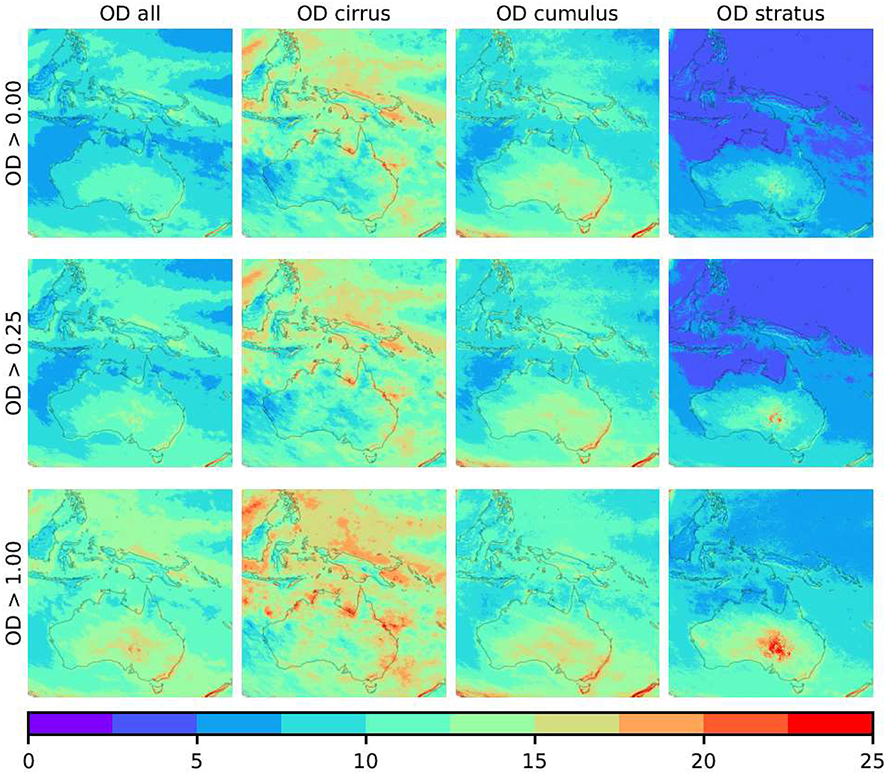
Figure 18. Change of yearly mean cloud optical depth (OD) with lower OD thresholds: the top row shows all data; the middle row only when OD > 0.25; and the bottom row when OD > 1.0. Data obtained for the period from 1 Jan 2016 to 30 Nov 2017 for daylight hours from 22UTC to 8UTC (8–18 Australian east standard time).

Conclusion

An algorithm for cloud masking, cloud classification and optical depth retrieval has been developed and applied to Himwari-8/AHI imagery. Cloud masking was performed using a time-series analysis that is based on the observation that the temporal variation of the surface (land and ocean) is much slower, on the scale of days-to-years, compared to that of the onset of clouds which change the TOA spectrum in the order of hours-to-minutes. A two-way confidence index has been developed, which measures either the cloudiness confidence, where the pixel is flagged cloudy, or the clearness confidence, where the pixel is flagged clear. By using this two-way confidence index it allows post-processing reclassification of pixels, to bias toward clearness or cloudiness depending on the application.

The cloud mask has been assessed using visual inspection and quantitatively validated using the Lidar sensor CALIOP. A direct comparison showed a hit rate—the proportion of pixels identified by both sensors as either clear or cloudy—of 87%. While geolocation differences (of about 1,400 m) played a minor role, this low hit rate is largely caused by the small footprint and sparse sampling of the CALIOP sensor under subpixel partial cloudy condition. Once cloud fraction was accounted for by only examining totally clear or overcast pixels, a hit rate of ~98% has been achieved even when the cloud optical depth was as low as 0.25.

Cloud classification and optical depth retrieval have been conducted based on radiative transfer modeling. The modeling error was found to be small. Qualitative analysis on classification examples has shown good consistency cloud texture and cloud top temperature. An indirect quantitative validation of retrieved cloud properties has been conducted by comparing surface solar flux calculated from the retrieved cloud properties with in-situ measurements, which showed excellent agreement between the two. The geographical cloud fraction generated from this study has been compared with ISCCP climatology, and the all-cloud-fraction showed agreement with that of ISCCP to a high degree, though some differences do exists in terms of some cloud types.

Despite the excellent outcomes in cloud detection, and very promising results in classification and optical depth retrieval, potential improvements are still possible. Currently, we concentrated on major factors affecting cloud detection and property retrieval, while minor but nevertheless potential issues were left for future work. Specifically, potential improvements could be achieved by: (i) taking into consideration of subpixel cloud fraction and cloud shadow which may lead to misclassification, particularly near cloud edges; (ii) incorporating a more realistic surface elevation; (iii) using latitude dependent atmosphere models to represent the molecular atmosphere for different latitude zones; (iv) considering surface BRDF which may have an effect on classification of thin clouds; (x) using longer wavelength bands to provide definitive distinguishing of aerosol from clouds, and (xi) handling of sun-glint over tropical oceans.

The data set generated is being used in a number of applications, including ocean color remote sensing, vegetation monitoring, solar energy, smoke detection for the studying of health impact, and aerosol and BRDF retrievals. For example, surface solar flux data generated using the cloud data (cloud type and optical depth) is being used in a new synergistic approach to solar energy forecasting on the time scales from minutes to days combining sky camera, satellite and numeric weather prediction model outputs. The quantified smoke plumes are being used to train a machine learning algorithm which can then be applied to other sensors including high resolution sensors. Due to the high temporal resolution of the AHI sensor (i.e., every 10 min), this cloud masking product provides the continuous cloud distribution over the region which can be used, for example, to flag cloud contamination in ground based measurements such as aerosols from sun photometers, or in imagery of other sensors, especially those with long revisit cycle where a time-series-based approach may not be suitable.

Author Contributions

All authors listed have made a substantial, direct and intellectual contribution to the work, and approved it for publication.

Conflict of Interest Statement

The authors declare that the research was conducted in the absence of any commercial or financial relationships that could be construed as a potential conflict of interest.

Acknowledgments

The authors would like to thank Dr John McGregor, CSIRO Oceans and Atmosphere Melbourne, for providing very constructive comments in an internal review. We also like to thank the two anonymous reviewers for their comments which helped substantially to improve the manuscript. This work was funded by CSIRO Oceans and Atmosphere as part of a collaborative project with the GCOM-C mission, JAXA. AHI images were provided by the Japanese Meteorology Agency through Australian Bureau of Meteorology. CALIOP cloud layer product was obtained from the NASA Langley Research Center. Surface-level solar flux measurements were acquired from Australian Bureau of Meteorology. Cloud climatology data were provided by the ISCCP project through https://www.ncei.noaa.gov/data/international-satellite-cloud-climate-project-isccp-h-series-data/access/isccp-basic/hgh/. Thanks to the Australian National Computational Infrastructure (NCI) and CSIRO Scientific Computing for providing essential computational resources and assistance.

References

Ackerman, S. A., Strabala, K. I., Menzel, W. P., Frey, R. A., Moeller, C. C., and Gumley, L. E. (1998). Discriminating clear sky from clouds with MODIS. J. Geophys. Res. Atmosp. 103, 32141–32157. doi: 10.1029/1998jd200032

CrossRef Full Text | Google Scholar

Austin, R. T., Heymsfield, A. J., and Stephens, G. L. (2009). Retrieval of ice cloud microphysical parameters using the CloudSat millimeter-wave radar and temperature. J. Geophys. Res. Atmosp. 114. doi: 10.1029/2008JD010049

CrossRef Full Text | Google Scholar

Baum, B. A., and Platnick, S. (2006). “Introduction to MODIS Cloud Products,” in Earth Science Satellite Remote Sensing, Vol. 1, Science and Instruments, eds J. J. Qu, W. Gao, M. Kafatos, R. E. Murphy, and V. V. Salomonson (Berlin; Heidelberg: Springer), 74–91.

Google Scholar

Beringer, J., Hutley, L. B., Abramson, D., Arndt, S. K., Briggs, P., Bristow, M., et al. (2015). Fire in Australian savannas: from leaf to landscape. Glob. Chang. Biol. 21, 62–81. doi: 10.1111/gcb.12686

PubMed Abstract | CrossRef Full Text | Google Scholar

Berk, A., Conforti, P., Kennett, R., Perkins, T., Hawes, F., and Bosch, J. V. D. (2014). “MODTRAN6: a major upgrade of the MODTRAN radiative transfer code,” in Algorithms and Technologies for Multispectral, Hyperspectral, and Ultraspectral Imagery XX (Baltimore, MD SPIE).

Google Scholar

Bessho, K., Date, K., Hayashi, M., Ikeda, A., Imai, T., Inoue, H., et al. (2016). An Introduction to Himawari-8/9-Japan's New-Generation Geostationary Meteorological Satellites. J. Meteorol. Soc. Jpn. 94, 151–183. doi: 10.2151/jmsj.2016-009

CrossRef Full Text | Google Scholar

BoM (2018). One Minute Solar Data. Available online at: http://reg.bom.gov.au/climate/reg/oneminsolar/index.shtml

Bowman, D. M. J. S., Balch, J. K., Artaxo, P., Bond, W. J., Carlson, J. M., Cochrane, M. A., et al. (2009). Fire in the earth system. Science 324, 481–484, doi: 10.1126/science.1163886

PubMed Abstract | CrossRef Full Text | Google Scholar

Chepfer, H., Bony, S., Winker, D., Cesana, G., Dufresne, J. L., Minnis, P., et al. (2010). The GCM-Oriented CALIPSO Cloud Product (CALIPSO-GOCCP). J. Geophys. Res. Atmosp, 115. doi: 10.1029/2009JD012251

CrossRef Full Text | Google Scholar

Dennekamp, M., Straney, L. D., Erbas, B., Abramson, M. J., Keywood, M., Smith, K., et al. (2015). Forest fire smoke exposures and out-of-hospital Cardiac Arrests in Melbourne, Australia: a case-crossover study. Environ. Health Perspect. 123, 959–964. doi: 10.1289/ehp.1408436

PubMed Abstract | CrossRef Full Text | Google Scholar

Donohue, R. J., McVicar, T. R., and Roderick, M. L. (2009). Climate-related trends in Australian vegetation cover as inferred from satellite observations, 1981–2006. Glob. Chang. Biol. 15, 1025–1039. doi: 10.1111/j.1365-2486.2008.01746.x

CrossRef Full Text | Google Scholar

Frey, R. A., Ackerman, S. A., Liu, Y., Strabala, K. I., Zhang, H., Key, J. R., et al. (2008). Cloud Detection with MODIS. Part I: Improvements in the MODIS Cloud Mask for Collection 5. J. Atmosp. Ocean. Technol. 25, 1057–1072. doi: 10.1175/2008jtecha1052.1

CrossRef Full Text | Google Scholar

Gomez-Chova, L., Amoros-Lopez, J., Mateo-Garcia, G., Munoz-Mari, J., and Camps-Valls, G. (2017). Cloud masking and removal in remote sensing image time series. J. Appl. Remote Sens. 11:15005. doi: 10.1117/1.Jrs.11.015005

CrossRef Full Text | Google Scholar

Haikerwal, A., Akram, M., Del Monaco, A., Smith, K., Sim, M. R., Meyer, M., et al. (2015). Impact of fine particulate matter (PM2.5) exposure during wildfires on cardiovascular health outcomes. J. Am. Heart Assoc. 4:e001653. doi: 10.1161/JAHA.114.001653

PubMed Abstract | CrossRef Full Text | Google Scholar

Heidinger, A. K., Foster, M. J., Walther, A., and Zhao, X. (2014). The pathfinder atmospheres–extended AVHRR climate dataset. Bull. Am. Meteorol. Soc. 95, 909–922. doi: 10.1175/bams-d-12-00246.1

CrossRef Full Text | Google Scholar

Hess, M., Koepke, P., and Schult, I. (1998). Optical properties of aerosols and clouds: the software package OPAC. Bull. Am. Meteorol. Soc. 79, 831–844. doi: 10.1175/1520-0477(1998)079<0831:Opoaac>2.0.Co;2

CrossRef Full Text | Google Scholar

Horsley, J. A., Broome, R. A., Johnston, F. H., Cope, M., and Morgan, G. G. (2018). Health burden associated with fire smoke in Sydney, 2001-2013. Med. J. Aust. 208, 309–310. doi: 10.5694/mja18.00032

PubMed Abstract | CrossRef Full Text | Google Scholar

Huang, C., Thomas, N., Goward, S. N., Masek, J. G., Zhu, Z., Townshend, J. R. G., et al. (2010). Automated masking of cloud and cloud shadow for forest change analysis using Landsat images. Int. J. Remote Sens, 31, 5449–5464. doi: 10.1080/01431160903369642

CrossRef Full Text | Google Scholar

Huang, J., Rikus, L. J., Qin, Y., and Katzfey, J. (2018). Assessing model performance of daily solar irradiance forecasts over Australia. Solar Ener. 176, 615–626, doi: 10.1016/j.solener.2018.10.080

CrossRef Full Text | Google Scholar

Hurst, D. F., Griffith, W. T., and Cook, G. D. (1994). Trace gas emissions from biomass burning in tropical Australian savannas. J. Geophys. Res. Atmosp. 99, 16441–16456. doi: 10.1029/94JD00670

CrossRef Full Text | Google Scholar

Hutchison, K. D., Heidinger, A. K., Kopp, T. J., Iisager, B. D., and Frey, R. A. (2014). Comparisons between VIIRS cloud mask performance results from manually generated cloud masks of VIIRS imagery and CALIOP-VIIRS match-ups. Int. J. Remote Sens. 35, 4905–4922. doi: 10.1080/01431161.2014.932465

CrossRef Full Text | Google Scholar

Hutchison, K. D., Roskovensky, J. K., Jackson, J. M., Heidinger, A. K., Kopp, T. J., Pavolonis, M. J., et al. (2005). Automated cloud detection and classification of data collected by the visible infrared imager radiometer suite (VIIRS). Int. J. Remote Sens, 26, 4681–4706. doi: 10.1080/01431160500196786

CrossRef Full Text | Google Scholar

Imai, T., and Yoshida, R. (2016). “Algorithm theoretical basis for himawari-8 cloud mask product,” in Meteorological Satellite Center Technical Note 61 (Tokyo: Japan Meteorolgical Agency), 1–17.

Google Scholar

Irish, R. R. (2000). “Landsat 7 automatic cloud cover assessment,” in AeroSense 2000 (Orlando, FL), 8. doi: 10.1117/12.410358:SPIE

CrossRef Full Text | Google Scholar

Iwabuchi, H., Putri, N. S., Saito, M., Tokoro, Y., Sekiguchi, M., Yang, P., et al. (2018). Cloud property retrieval from multiband infrared measurements by Himawari-8. J. Meteorol. Soc. Jpn. 96b, 27–42. doi: 10.2151/jmsj.2018-001

CrossRef Full Text | Google Scholar

Karlsson, K. G., and Hakansson, N. (2018). Characterization of AVHRR global cloud detection sensitivity based on CALIPSO-CALIOP cloud optical thickness information: demonstration of results based on the CM SAF CLARA-A2 climate data record. Atmosp. Measur. Tech. 11, 633–649. doi: 10.5194/amt-11-633-2018

CrossRef Full Text | Google Scholar

Koner, P. K., Harris, A., and Maturi, E. (2016). Hybrid cloud and error masking to improve the quality of deterministic satellite sea surface temperature retrieval and data coverage. Remote Sens. Environ, 174, 266–278. doi: 10.1016/j.rse.2015.12.015

CrossRef Full Text | Google Scholar

Kopp, T. J., Thomas, W., Heidinger, A. K., Botambekov, D., Frey, R. A., Hutchison, K. D., et al. (2014). The VIIRS cloud mask: progress in the first year of S-NPP toward a common cloud detection scheme. J. Geophys. Res. Atmosp. D119, 2441–2456. doi: 10.1002/2013jd020458

CrossRef Full Text | Google Scholar

Lee, J. S. (1986). Speckle suppression and analysis for synthetic aperture radar images. Opt. Eng. 25, 636–643.

Google Scholar

Liao, X. H., Rossow, W. B., and Rind, D. (1995). Comparison between Sage-Ii and Isccp High-Level Clouds.1. Global and Zonal Mean Cloud Amounts. J. Geophys. Res. Atmosp. D100, 1121–1135. doi: 10.1029/94jd02429

CrossRef Full Text | Google Scholar

Liou, K.-N. (1980). An introduction to Atmosphere Radiation, 1 Edn. New York, NY: Academic Press.

Google Scholar

Lyapustin, A., Wang, Y., and Frey, R. (2008). An automatic cloud mask algorithm based on time series of MODIS measurements. J. Geophys. Res. Atmosp. D113. doi: 10.1029/2007jd009641

CrossRef Full Text | Google Scholar

Massie, S., Gettelman, A., Randel, W., and Baumgardner, D. (2002). Distribution of tropical cirrus in relation to convection. J. Geophys. Res. Atmosp. D107. doi: 10.1029/2001jd001293

CrossRef Full Text | Google Scholar

McVicar, T. R., and Jupp, D. L. B. (1999). Estimating one-time-of-day meteorological data from standard daily data as inputs to thermal remote sensing based energy balance models. Agric. Forest Meteorol. 96, 219–238. doi: 10.1016/S0168-1923(99)00052-0

CrossRef Full Text | Google Scholar

Mernagh, T. P. (2013). A Review of Australian Salt Lakes and Assessment of Their Potential for Strategic Resources. Report 2013/39, Geoscience, Canberra, ACT.

Mitchell, R. M., Forgan, B., and Campbell, S. K. (2017). The climatology of Australian Aerosol. Atmosp Chem Phys. 17, 5131–5154. doi: 10.5194/acp-17-5131-2017

CrossRef Full Text | Google Scholar

Nakajima, T., and Tanaka, M. (1986). Matrix formulations for the transfer of solar-radiation in a plane-parallel scattering atmosphere. J. Quant. Spectros. Radiat. Transf. 35, 13–21. doi: 10.1016/0022-4073(86)90088-9

CrossRef Full Text | Google Scholar

NOAA (2018). International Satellite Cloud Climatology Project (ISCCP) H-series Data. Available online at: https://www.ncei.noaa.gov/data/international-satellite-cloud-climate-project-isccp-h-series-data/access/isccp-basic/hgh/

O'Keeffe, D., Dennekamp, M., Straney, L., Mazhar, M., O'Dwyer, T., Haikerwal, A., et al. (2016). Health effects of smoke from planned burns: a study protocol. BMC Public Health 16:186. doi: 10.1186/s12889-016-2862-y

PubMed Abstract | CrossRef Full Text | Google Scholar

Qin, Y., and Box, M. A. (2005). Analytic green's function for radiative transfer in plane-parallel atmospheres. J. Atmosp. Sci. 62, 2910–2924. doi: 10.1175/jas3532.1

CrossRef Full Text | Google Scholar

Qin, Y., and Box, M. A. (2006). Vector Green's function algorithm for radiative transfer in plane-parallel atmosphere. J. Quant. Spectros. Radiat. Transf. 97, 228–251. doi: 10.1016/j.jqsrt.2005.04.009

CrossRef Full Text | Google Scholar

Qin, Y., Mitchell, R., and Forgan, B. W. (2015). Characterizing the aerosol and surface reflectance over Australia using AATSR. IEEE Trans. Geosci. Remote Sens. 53, 6163–6182. doi: 10.1109/Tgrs.2015.2433911

CrossRef Full Text | Google Scholar

Qin, Y., and Mitchell, R. M. (2009). Characterisation of episodic aerosol types over the Australian continent. Atmosp. Chem. Phys. 9, 1943–1956. doi: 10.5194/acp-9-1943-2009

CrossRef Full Text | Google Scholar

Rossow, W. B., and Schiffer, R. A. (1999). Advances in Understanding Clouds from ISCCP. Bull. Am. Meteorol. Soc. 80, 2261–2288. doi: 10.1175/1520-0477(1999)080<2261:Aiucfi>2.0.Co;2

CrossRef Full Text | Google Scholar

Sassen, K., and Wang, Z. (2008). Classifying clouds around the globe with the CloudSat radar: 1-year of results. Geophys. Res. Lett. 35. doi: 10.1029/2007GL032591

CrossRef Full Text | Google Scholar

Sassen, K., Wang, Z., and Liu, D. (2008). Global distribution of cirrus clouds from CloudSat/Cloud-Aerosol Lidar and Infrared Pathfinder Satellite Observations (CALIPSO) measurements. J. Geophys. Res. Atmosp. D113. doi: 10.1029/2008jd009972

CrossRef Full Text | Google Scholar

Sassen, K., Wang, Z., and Liu, D. (2009). Cirrus clouds and deep convection in the tropics: insights from CALIPSO and CloudSat. J. Geophys. Res. Atmosp. D114. doi: 10.1029/2009jd011916

CrossRef Full Text | Google Scholar

Saunders, R. W. (1986). An automated scheme for the removal of cloud contamination from Avhrr radiances over Western-Europe. Int. J. Remote Sens. 7, 867–886. doi: 10.1080/01431168608948896

CrossRef Full Text | Google Scholar

Schulz, J., Albert, P., Behr, H. D., Caprion, D., Deneke, H., Dewitte, S., et al. (2009). Operational climate monitoring from space: the EUMETSAT Satellite Application Facility on Climate Monitoring (CM-SAF). Atmosp. Chem. Phys. 9, 1687–1709. doi: 10.5194/acp-9-1687-2009

CrossRef Full Text | Google Scholar

Stengel, M., Stapelberg, S., Sus, O., Schlundt, C., Poulsen, C., Thomas, G., et al. (2017). Cloud property datasets retrieved from AVHRR, MODIS, AATSR and MERIS in the framework of the Cloud_cci project. Earth Syst. Sci. Data 9, 881–904. doi: 10.5194/essd-9-881-2017

CrossRef Full Text | Google Scholar

Stephens, G. L. (2005). Cloud feedbacks in the climate system: a critical review. J. Clim. 18, 237–273. doi: 10.1175/jcli-3243.1

CrossRef Full Text | Google Scholar

Stephens, G. L., and Kummerow, C. D. (2007). The remote sensing of clouds and precipitation from space: a review. J. Atmosp. Sci., 64, 3742–3765. doi: 10.1175/2006jas2375.1

CrossRef Full Text | Google Scholar

Stowe, L. L., Davis, P. A., and McClain, E. P. (1999). Scientific basis and initial evaluation of the CLAVR-1 global clear cloud classification algorithm for the advanced very high resolution radiometer. J. Atmosp. Oceanic Technol. 16, 656–681. doi: 10.1175/1520-0426(1999)016<0656:Sbaieo>2.0.Co;2

CrossRef Full Text | Google Scholar

Stubenrauch, C. J., Cros, S., Guignard, A., and Lamquin, N. (2010). A 6-year global cloud climatology from the Atmospheric InfraRed Sounder AIRS and a statistical analysis in synergy with CALIPSO and CloudSat. Atmosp. Chem. Phys. 10, 7197–7214. doi: 10.5194/acp-10-7197-2010

CrossRef Full Text | Google Scholar

Stubenrauch, C. J., Feofilov, A. G., Protopapadaki, S. E., and Armante, R. (2017). Cloud climatologies from the infrared sounders AIRS and IASI: strengths and applications. Atmosp. Chem. Phys. 17, 13625–13644. doi: 10.5194/acp-17-13625-2017

CrossRef Full Text | Google Scholar

Stubenrauch, C. J., Rossow, W. B., Kinne, S., Ackerman, S., Cesana, G., Chepfer, H., et al. (2013). Assessment of global cloud datasets from satellites: project and database initiated by the GEWEX Radiation Panel. Bull. Am. Meteorol. Soc. 94, 1031–1049. doi: 10.1175/Bams-D-12-00117.1

CrossRef Full Text | Google Scholar

Sun, W. B., Videen, G., and Mishchenko, M. I. (2014). Detecting super- thin clouds with polarized sunlight. Geophys. Res. Lett. 41, 688–693. doi: 10.1002/2013gl058840

CrossRef Full Text | Google Scholar

Vermote, E. F., Tanre, D., Deuze, J. L., Herman, M., and Morcrette, J. J. (1997). Second Simulation of the Satellite Signal in the Solar Spectrum, 6S: an overview. IEEE Trans. Geosci. Remote Sens. 35, 675–686. doi: 10.1109/36.581987

CrossRef Full Text | Google Scholar

Walther, A., Straka, W., and Heidinger, A. K. (2011). ABI Algorithm Theoretical Basis Document for Daytime Cloud Optical and Microphysical Properties (DCOMP), version 2.0. NOAA/NESDIS/Center for Satellite Applications and Research, 61 pp. Available online at: http://www.goes-r.gov/products/ATBDs/baseline/Cloud_DCOMP_v2.0_no_color.pdf

Wang, P. H., Minnis, P., McCormick, M. P., Kent, G. S., and Skeens, K. M. (1996). A 6-year climatology of cloud occurrence frequency from stratospheric aerosol and gas experiment II observations (1985-1990). J. Geophys. Res. Atmosp. D101, 29407–29429. doi: 10.1029/96jd01780

CrossRef Full Text | Google Scholar

Wang, T., Fetzer, E. J., Wong, S., Kahn, B. H., and Yue, Q. (2016). Validation of MODIS cloud mask and multilayer flag using CloudSat-CALIPSO cloud profiles and a cross-reference of their cloud classifications. J. Geophys. Res. Atmosp. D121, 11620–11635. doi: 10.1002/2016jd025239

CrossRef Full Text | Google Scholar

Wang, Z., Wang, Z. H., Cao, X. Z., and Tao, F. (2018). Comparison of cloud top heights derived from FY-2 meteorological satellites with heights derived from ground-based millimeter wavelength cloud radar. Atmosp. Res. 199, 113–127. doi: 10.1016/j.atmosres.2017.09.009

CrossRef Full Text | Google Scholar

Winker, D. (2016). CALIPSO LID_L2_01kmCLay-Standard HDF File. Version 4.10. NASA Langley Atmospheric Science Data Center DAAC.

Winker, D. M., Vaughan, M. A., Omar, A., Hu, Y., Powell, K. A., Liu, Z., et al. (2009). Overview of the CALIPSO mission and CALIOP data processing algorithms. J. Atmosp. Oceanic Technol. 26, 2310–2323. doi: 10.1175/2009jtecha1281.1

CrossRef Full Text | Google Scholar

Wood, R. (2012). Stratocumulus clouds. Mon. Weather Rev. 140, 2373–2423. doi: 10.1175/mwr-d-11-00121.1

CrossRef Full Text | Google Scholar

Yang, J., Gong, P., Fu, R., Zhang, M. H., Chen, J. M., Liang, S. L., et al. (2013). The role of satellite remote sensing in climate change studies. Nat. Clim. Chang. 3, 875–883. doi: 10.1038/Nclimate1908

CrossRef Full Text | Google Scholar

Yuter, S. E., Hader, J. D., Miller, M. A., and Mechem, D. B. (2018). Abrupt cloud clearing of marine stratocumulus in the subtropical southeast Atlantic. Science 17, 697–701. doi: 10.1126/science.aar5836

CrossRef Full Text | Google Scholar

Zhang, Y., Rossow, W. B., Lacis, A. A., Oinas, V., and Mishchenko, M. I. (2004). Calculation of radiative fluxes from the surface to top of atmosphere based on ISCCP and other global data sets: refinements of the radiative transfer model and the input data. J. Geophys. Res. Atmosp. 109. doi: 10.1029/2003JD004457

CrossRef Full Text | Google Scholar

Zhao, B., Gu, Y., Liou, K. N., Wang, Y., Liu, X., Huang, L., et al. (2018). Type-dependent responses of ice cloud properties to aerosols from satellite retrievals. Geophys. Res. Lett. 45. doi: 10.1002/2018GL077261

CrossRef Full Text | Google Scholar

Zou, X. L., and Da, C. (2014). An objective regional cloud mask algorithm for GOES infrared imager radiance assimilation. J. Geophys. Res. Atmosp. D119, 6666–6680. doi: 10.1002/2014jd021455

CrossRef Full Text | Google Scholar