Generating a Set of Temperature Time Series Representative of Recent Past and Near Future Climate

Introduction

The climate and energy systems are closely interrelated; future changes in the climate are likely to drive changes in energy systems (e.g., increased air temperatures requiring more energy for cooling purposes) and developments in the energy sector (e.g., greater use of renewable energy and storage technology) will help to decarbonize the economy. The intimate link between weather and energy is fully discussed in a recent book (Troccoli et al., 2014; Añel, 2015). Bossmann and Staffell (2015) studied the possible changes in electricity demand due to different changes in electricity use in the future linked to climate change mitigation. Due to the importance of heating and cooling, temperature will remain, an important driver of electricity demand. McFarland et al. (2015) studied the impact of temperature increase on electricity supply and demand in the United States, by applying temperature projections to three electric sector models in the US. In Europe, the historical link between electricity demand and temperature is not linear, and three types of countries can be identified (Bessec and Fouquau, 2008): cold countries which only exhibit a heating effect, intermediate countries with a dominant heating effect and a small cooling effect and warm countries which clearly exhibit both effects. France is an intermediate country in that respect. The study also provides evidence of an increase in the sensitivity to temperature during the summer in recent years. In warm European countries, global warming combined with the urban heat island effect may have a major impact on electricity consumption (see (Santamouris et al., 2015) for a review). Besides average load changes, changes in peak demand are of importance for the design of peak load management strategies (storage, demand side management, interconnection, and peaking capacities). Peak demand may be linked to severe weather conditions like heat waves and cold waves. For example, during the February 2012 cold wave (Luo et al., 2014), French electricity consumption reached a new record exceeding the value from winter 2010 by 5 GW and the 10 years old previous one by more than 20 GW (RTE, 2012); this record most likely occurred due to electrical heating in buildings. Añel et al. (2017) detail the impacts of heat waves and cold waves on the energy sector with the help of historical events. The impact of climate change on the frequency and intensity of peak electricity demand has been studied by Auffhammer et al. (2017) for the US. They derived statistical models for the link of base and peak electricity demand with temperature. They used 20 downscaled General Circulation Model outputs to project climate change induced base and peak load changes, and showed that the impact on peak load well exceeds that on base load.

As heat waves and cold waves are rare events, their frequency can only be estimated from very large samples. To study how climate change could have modified the probability of occurrence of a recent cold event in Spain, Añel et al. (2017) analyzed the very large ensemble of climate projections produced by the Weatherathome.net project (Massey et al., 2014). The ensemble is based on only one pair of general and regional circulation models (HadAM3/HadRM3P) and cannot explore the large range of uncertainties in climate projections due to model differences. The aim of this study is to test another way of generating large ensembles of possible evolutions in order to study changes in the frequency of heat waves and cold waves. The approach is based on a combination of observations and climate projections with a stochastic weather generator.

Weather generators for temperature have commonly been used for pricing derivatives in the energy sector (Campbell and Diebold, 2005; Mraoua and Bari, 2007; Benth and Saltyte Benth, 2011); research in the fields of agriculture and hydrology have also extended the use of weather generators. In those models, the simulation of temperature is generally conditioned on the occurrence of rainfall. The most widely used models of such type are based on the concept proposed by Richardson (1981) that the standardized residuals of temperature are assumed normally distributed, and the coefficients of the model are estimated using autocorrelations and cross-correlations between the residuals of the different variables involved. Then, the removed means and standard deviations are reintroduced, depending on whether the day is dry or wet. More recently, the use of Generalized Linear Models (GLM) in weather generators have been increasing, since they allow a better treatment of non-linearity and can model discrete and non-normally distributed variables. GLMs are also useful to handle the El Niño-Southern Oscillation (ENSO) and other modes of variability (Chandler, 2005; Furrer and Katz, 2007). Acknowledging both the usefulness and limitations of Richardson type generators, Smith et al. (2017) recently proposed an extension called SHArP (Stochastic Harmonic Autoregressive Parametric weather generator), used to generate temperature time series. The proposed model framework allows for trends and seasonality in the temperature generation.

In these studies using weather generators, the impact of climate change is generally taken into account using Change Factors (CFs). The CFs express the changes between a baseline climate and future projections. They are applied to the statistics of the observed time series to produce projected time series. Then, these projected time series are used to calibrate the weather generator. Glenis et al. (2015) used such a technique to provide large samples of time series allowing the exploration of natural variability and climate model uncertainties in a study of water resources management strategies in a non-stationary climate. Smith et al. (2017) built a continuous temperature time series between 1948 and 2100 by linking observations with a bias adjusted climate model simulation. This time series is then used to fit the generator and produce a larger sample. Here again, only one climate model is considered.

As stated previously, the goal of this paper is to produce a large sample of a temperature based indicator by mixing observations, climate projections and stochastic generation to analyze the changes in the frequency of heat waves and cold waves in France due to climate change. This study makes use of another type of stochastic generator and an ensemble of climate projections with different climate models is considered. The stochastic generator relies on the decomposition of the temperature signal into deterministic parts (seasonality and trends in the mean and the standard deviation) and a stochastic part, which is represented by a Seasonal Functional Heteroscedastic Autoregressive (SFHAR) model (Parey et al., 2014; Dacunha-Castelle et al., 2015). The trend components are then changed using climate model simulations to generate a large sample of thermal indicator time series covering the recent past and the near future. In section Data and Methodology the temperature dataset used to compute the indicator will be introduced alongside the principles of the generator. A test of the proposed approach in a cross-validation setting will be detailed in section Test in a Cross-Validation Setting, with a focus on the reproduction of severe heat waves and cold waves. In section Application to the Production of Possible 1981–2040 Trajectories the generation will be extended to the next decades, with a first estimate of the changes in frequency of the most intense historical heat waves and cold waves provided. Section Discussion and Perspectives provides a discussion and conclusion.

Data and Methodology

The Thermal Indicator

Models used for mid-term load forecasting at Electricité de France (EDF) are based on past values of load, temperature, date, and calendar events (Bruhns et al., 2005). In these models, the influence of temperature is estimated through a thermal indicator computed as a weighted average of the observed temperature at 32 locations across the country; the weights are representative of the share of the electricity demand that each city represents in the nationwide total. The 32 locations are cities where stations of the Météo-France observation network are located. They are listed in Table 1 together with their associated longitude, latitude, altitude, and weight (for the weighted average), and illustrated in Figure 1. The observation periods are different for the different stations, so to be able to study this indicator for a long period, it is computed from the daily mean temperature of the E-OBS gridded dataset (Haylock et al., 2008) by selecting the nearest grid point to each station and correcting for the altitude difference between the selected point and the station. The altitude correction is based on the standard atmosphere temperature gradient of 6.5°C/km, and the weighted average is computed as:

$\begin{array}{l}X(t)={{\displaystyle \sum }}_{s=1}^{32}w(s)T(s,t),\end{array}$

with T(s, t) the temperature on day t in station s and. w(s) the weight of each station. Since temperature is highly spatially correlated in the domain, the averaging does not smooth out temporal variability.

TABLE 1

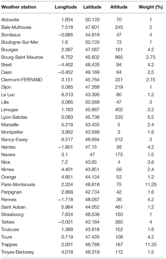
Table 1. Weather stations for the temperature used to compute the thermal indicator for electricity demand in France, with their associated longitudes, latitudes, altitudes, and weights in the weighted average.

FIGURE 1

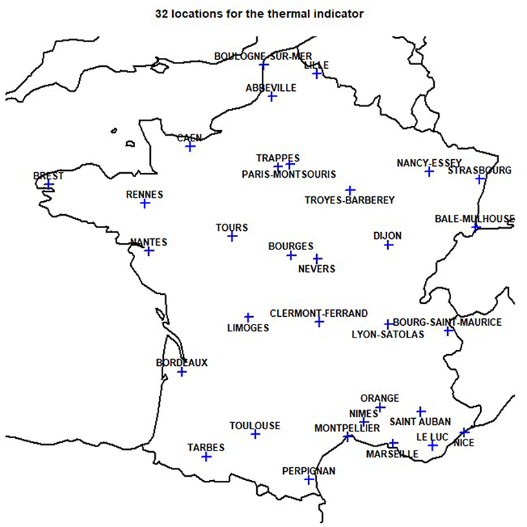
Figure 1. Location of the 32 weather stations used to compute the thermal indicator for the electricity demand in France.

This produces one daily time series of weighted average temperatures covering the period 1950–2017 which is called the thermal indicator. This is not exactly the temperature indicator used for electricity demand, which is based on the three-hourly observed temperature datasets at each Météo-France station, but it has been checked that the obtained time series is fairly close to this indicator if considered at the daily time scale: the mean absolute difference is around 0.3°C and the correlation over the common period 1980–2009 is 0.997.

In this daily time series of the thermal indicator in France from 1950 to 2017, the observed minimum is −10.2°C on 2nd February 1956 and the observed maximum is 28.7°C on 5th August 2003. For the rest of this paper, comparisons will focus on heat waves and cold waves. The World Meteorological Organization (WMO) does not provide any standard definition for these events. Therefore, they are defined here as a number of consecutive days with a thermal indicator lower (for cold waves) or higher (for heat waves) than a low or high threshold. The chosen thresholds are respectively, the (rounded) 2nd and 98th percentile of the thermal indicator distribution: 0°C for the cold waves and 23°C for the heat waves. Then, each event is characterized by its duration and its intensity, this last quantity being estimated as the summation of the differences to the threshold across the whole event. The intensity is thus positive for heat waves and negative for cold waves. The five most intense events in the total observed period, and in sub-periods 1955–1986 and 1987–2017, which will be considered in the study, are summarized in Table 2. One can identify the well-known cold winters of 1956, 1963, 1985, and 1987 and hot summers of 1976, 1983, 1990, 2003, 2006, and 2015. It is interesting to note that the most intense cold events occurred in the first sub-period and the most intense hot events in the second sub-period. This is consistent with the last IPCC assessment report stating as very likely that the frequency of cold days has decreased and the frequency of hot days has increased in the recent decades (IPCC, 2013).

TABLE 2

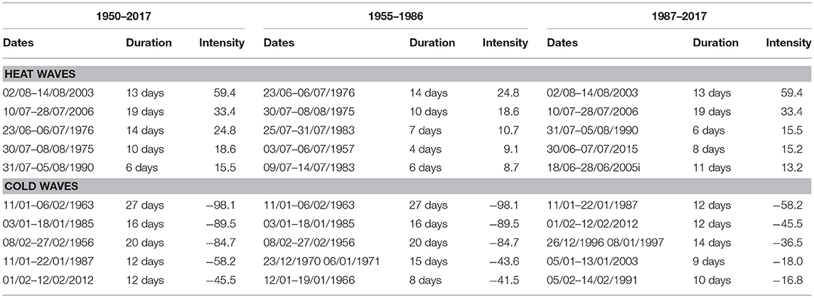
Table 2. Five most intense heat and cold waves observed for the three periods considered.

Climate Model Simulations

Projections of the thermal indicator for the coming decades are obtained from climate model simulations. The simulations used here have been extracted from the IPCC AR5 simulation database and gather 23 model simulations with emission scenario RCP8.5. The list of the considered models is given in Table 3, and only one run (the first one) is considered when more than one simulation is available for a particular model over the same period so that each model shares the same weight in the ensemble. Then, in the same way as for the E-OBS gridded dataset, the thermal indicator is computed from the daily mean temperature time series of the nearest grid point to the 32 observation stations. The weighted 32-station averages are thus computed for each model simulation over the period 1955–2100, which is the common period for all the retrieved model simulations.

TABLE 3

Table 3. Climate model simulations used in the study.

Methodology

The Temperature Generator

A SFHAR generator previously developed at EDF/R&D is used to produce a large sample of this temperature indicator mentioned above. The principle and mathematical justifications of the generator are detailed in Dacunha-Castelle et al. (2015), and only a brief description will be given here.

The temperature based indicator is modeled in the following way:

$\begin{array}{l}X(t)=m(t)+S(t)+s(t)S_{sd}(t)Z(t)\end{array}$

where X(t) represents the indicator on day t, m(t), and s(t) are non-parametric trends in mean and standard deviation, S(t) and S_sd(t) are the seasonality of the mean and the standard deviation, respectively, and Z(t) is the noise sequence. The aim of such decomposition is to remove the deterministic parts of the signal and design a generator for the stochastic part Z(t).

The non-parametric trends are estimated using a degree 1 local regression using the LOESS technique (Stone, 1977). The choice of the smoothing parameter is based on a modified partitioned cross-validation approach developed in Hoang (2010). The classical partitioned cross-validation technique of Marron (1987) had to be modified because the variance is not constant.

The seasonality is estimated by a trigonometric polynomial of the form:

$\begin{array}{l}{\theta }_0+{{\displaystyle \sum }}_{i=1}^p\left({\theta }_{i,1}cos\left(\frac{2\pi it}{365}\right)+{\theta }_{i,2}sin\left(\frac{2\pi it}{365}\right)\right)\end{array}$

with parameters θ₀, θ_{i, 1}, and θ_{i, 2} obtained by least squares fitting. The degree p is chosen according to an Akaike criterion.

Hoang (2010) showed that if the same smoothing parameters are used, estimating seasonality first, then trend, gives the same results as estimating trend first then seasonality. However, the optimal smoothing parameter may not be the same depending whether the estimation of the trends is made first or second. Furthermore, if seasonality is estimated first, some part of the trend is embedded in the mean seasonality. Therefore, in this study, trend will be estimated first, then seasonality. Besides, considering non-parametric trends rather than linear ones allows us to take into account both the warming effect and some part of interannual to decadal variability.

Once the trends and seasonality are estimated, the elements of the noise sequence are estimated through the expression:

$\widehat{Z}\left(t\right)=\frac{X\left(t\right)-\widehat{m}\left(t\right)-\widehat{S}(t)}{\widehat{s}(t)\widehat{S_{sd}}(t)}\text{ where the hat denotes an estimator}.$

The process of Z(t) has been carefully studied in Hoang (2010). Based on permutation tests, it has been shown that its mean, variance, skewness, kurtosis, as well as its first and second order autocorrelations do not show any trend. A stationarity test based on simulation has also been used to check that trends are not detected in the tails of its distribution. The details of the tests can be found in Dacunha-Castelle et al. (2015). Since the process is Markovian and cyclo-stationary with an annual period, it can be considered as provided by a cyclo-stationary diffusion. The proposed SFHAR representation corresponds to the first order Euler scheme approximation of the diffusion for discrete variables (see (Dacunha-Castelle et al., 2015) for the demonstrations). The model is expressed by the following equation:

$\begin{array}{l}Z(t)=b_{t}Z(t-1)+a(t,Z(t-1)){\epsilon }_t\text{with }{\epsilon }_t\text{ a standard}\\ \text{normal distribution}.\end{array}$

The auto regression coefficient b_t is seasonal, and is estimated in the same way as previously by a trigonometric polynomial whose degree is chosen according to an Akaike criterion. The volatility a is represented by a degree 5 trigonometric polynomial of the form:

$\begin{array}{lll}\hfill a^2(t,Z(t-1))& =& (r_2-t)(t-r_1){{\displaystyle \sum }}_{k=0}^5{{\displaystyle \sum }}_{j=1}^{p_2}\\ & & \left({\alpha }_{1,k}^{j}cos\left(\frac{2\pi jt}{365}\right)+{\alpha }_{2,k}^{j}sin\left(\frac{2\pi jt}{365}\right)\right){Z\left(t-1\right)}^k\end{array}$

with constraints on the derivatives so that a² is positive and is zero outside the interval [r₁,r₂], with r₁ and r₂ being the lower and upper bounds of its distribution. The lower and upper bounds are estimated by fitting a Generalized Extreme Value (GEV) distribution to the block minima and maxima, respectively: ${\widehat{r}}_1={\widehat{\mu }}_1-\frac{{\widehat{\sigma }}_1}{{\widehat{\xi }}_1}$ and ${\widehat{r}}_2={\widehat{\mu }}_2-\frac{{\widehat{\sigma }}_2}{{\widehat{\xi }}_2}$ with ${\widehat{\mu }}_1,{\widehat{\sigma }}_1,{\widehat{\xi }}_1$ and ${\widehat{\mu }}_2,{\widehat{\sigma }}_2,{\widehat{\xi }}_2$ being, respectively, the estimated parameters of the GEV distribution fitted to the block minima and to the block maxima of Z(t). In practice, the autoregressive part of Z(t) is estimated first, then a is estimated from (Z(t) − b_tZ(t − 1))² by maximum likelihood with constraints. Firstly, the degree (p₂) of the trigonometric polynomial is chosen following an Akaike criterion and a is estimated by least squares with constraints, using the algorithm in Golfarb and Idnani (1982) and Godfarb and Idnani (1983). Then the results of the least square estimation are used as the initial values for the parameters in the likelihood maximization. The estimation of a² is obtained by using the algorithm of Nelder and Mead (1965). Lastly, a² is zero outside the interval (${\widehat{r}}_1$; ${\widehat{r}}_2$).

In the following, the time series characterizing the evolution of the thermal indicator over different time periods will be equally named time series or trajectories.

Building the Trajectories

In France, peak loads occur in winter during intense cold waves (RTE, 2012). Therefore, a large sample is needed to estimate frequencies and frequency changes in the most severe events. Furthermore, even though the sensitivity in summer is much lower, anticipating the changes in the frequency of the most intense heat waves is of interest too, because hot events may lead to a reduction in the generation from thermal plants due to increases in the temperature of water used for cooling (Troccoli et al., 2014; Añel, 2015).

The idea here is to take advantage of the previously described generator to produce the desired large sample of indicator trajectories. Since the residuals simulated by the generator have been proven to be stationary with an annual periodicity, they can be used to build trajectories for different time periods, both historical and future. Under the assumption that the typical signal for a period essentially lies in the trends of both the mean and the standard deviation, a sample of trajectories for a chosen period can be obtained by combining observed seasonality, projected trends and a large number of simulations of the residuals given by the generator. The assumption is reasonable, as illustrated in Figure 2 which compares trends and seasonality of the indicator in the period 1955–1986 and in the full period 1950–2017. The projected trends are provided by climate model simulations.

FIGURE 2

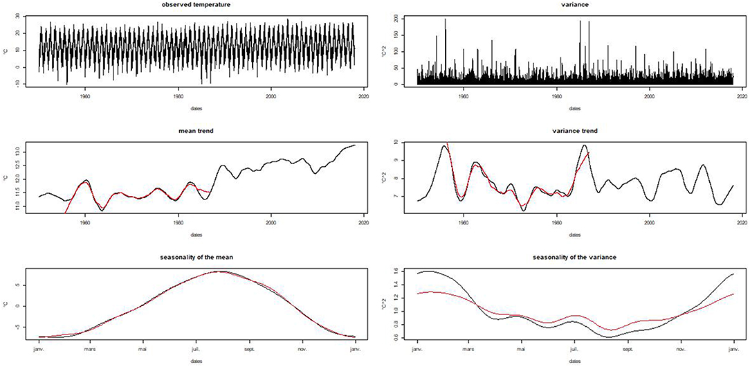
Figure 2. Observed indicator from 1950 to 2017 (top left panel), non-parametric trend in mean (middle left panel), seasonality of the mean (bottom left panel), evolution of the variance (top right panel), non-parametric trend in variance (middle right panel), and seasonality of the variance (bottom right panel). Black curves are for the total period and red curves for period 1955–1986.

Test in a Cross-Validation Setting

To test the proposed methodology and its associated assumptions, two periods of equivalent length are chosen from the observation period: 1955–1986 and 1987–2017. The proposed methodology is then used to build trajectories covering the whole period 1955–2017 (63 years) in the following way:

– Computation of Z(t) from the observations in period 1955–1986

– Simulation of a large number of 63-years trajectories of Z(t) with the generator

– Retrieval of the trends in mean and standard deviation for the period 1955–2017 from the climate models

– Reconstruction of a large number of trajectories for the period 1955–2017 by combining the Z(t) trajectories with the observed seasonalities and the climate model trends.

The sensitivity of the reconstruction to different choices [climate model, smoothing parameter for the trends, number of Z(t) trajectories] is investigated and validated against the observations in period 1987–2017 with a special focus on heat and cold waves.

Calibration

The approach is first calibrated over the period 1955–1986. Figure 3 illustrates the decomposition of the indicator in the period 1955–1986. The residuals Z(t) are estimated and used to fit the generator, which is then used to produce a large sample of 500 63-years trajectories of equivalent residuals.

FIGURE 3

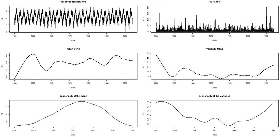
Figure 3. Same as Figure 2 but for period 1955–1986 only.

The construction of a 63-years thermal indicator time series in the period 1955–2017 requires the replacement of the observed trends in mean and standard deviation of the indicator over period 1955–1986 by similar trends over the total period 1955–2017 given by the climate models. In a first step, to estimate the sensitivity to the choice of climate model, four climate simulations have been selected. The selection is based on Boé (2018) who studied the interdependency of the climate models in the last CMIP5 exercise. Among the 23 simulations used in this study, four models presenting different representations for each of the four components (atmosphere, ocean, land, and ice) are first selected: BNU-ESM, IPSL-CM5-MR, MIROC5, and MPI-ESM-MR. Then, the indicator time series over period 1955–2017 obtained from each of the four models are decomposed and the trends in mean and standard deviation are bias adjusted to the observed trends. The bias adjustment is made for the period 1955–1986 only and is a simple mean bias removal. The obtained trends are illustrated together with the observed ones in Figure 4. Finally, 500 indicator time series are built using these bias adjusted trends, the observed seasonality and the 500 simulations of the residuals for each of the four models, which leads to 2000 63-years trajectories.

FIGURE 4

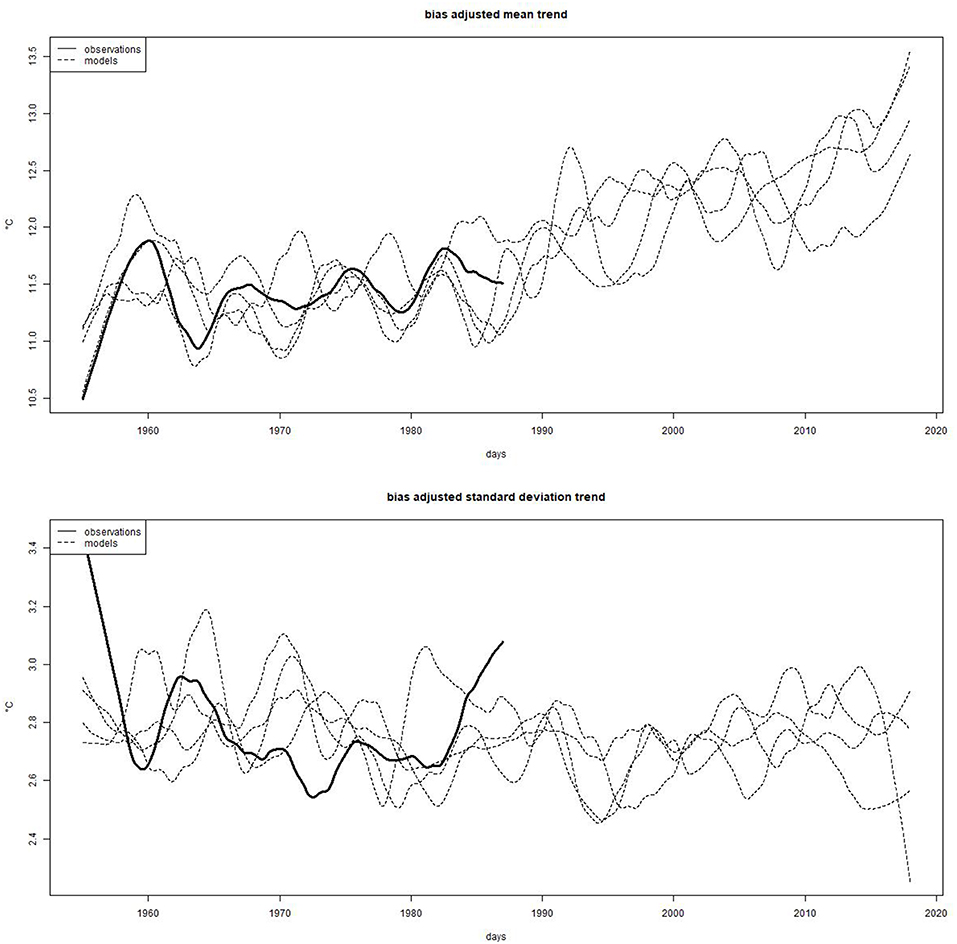
Figure 4. Bias adjusted trends in mean (top panel) and standard deviation (bottom panel) extracted from four climate model simulations (dotted lines) with the observed trends in the calibration period 1955–1986 (black line).

Validation

A check has been made that the observed mean annual cycle over the total period 1955–2017 lies inside the minimum and maximum mean annual cycles of the 2000 trajectories. Figure 5 shows that this is the case.

FIGURE 5

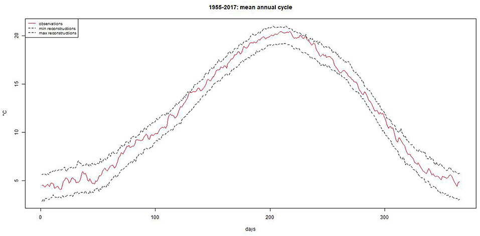
Figure 5. Observed mean annual cycle in the total period 1955–2017 (red line) compared to the envelope of the mean annual cycles in the same period from the reconstructions (dotted lines).

Then, as the focus here is on heat waves and cold waves, the number and intensities of these events over each period (i.e., calibration period 1955–1986 and validation period 1987–2017) are compared. The observed maximum number of events and the observed maximum intensity each year is compared to the 90% confidence interval of the same quantities in the simulations (the 90% confidence interval's lower and upper bounds are respectively, the 5th and 95th percentile of the distribution given by the 2000 simulations). Figure 6 shows the results for the yearly maximum number of events (left panels) and the yearly maximum intensity (right panels) for heat waves and cold waves in 1955–1986 (first two lines) and in 1987–2017 (last two lines). Statistically, one can expect that 5% of the observed maximum numbers or intensities of events exceed the upper bound or the lower bound of the 90% confidence interval. Period 1955–1986 is 32 years long and period 1987–2017 31 years long, which means that observations may lie outside the interval around 1.5–1.6 times for each series. Figure 6 shows that broadly this is what happens in the period 1955–1986 while in the period 1987–2017 the observed maximum number of heat waves exceeds the 90% upper bound four times. However, the intensity of the heat waves are correctly represented, since only two exceed the upper bound of the 90% confidence interval. To check if this could be due to the differences in trends between model and observations, the same estimates have been provided but for trajectories constructed with the observed trends over the whole 1955–2017 period. In that case too, four exceedances occur in the period 1987–2017 for the number of heat waves. These results show that the reconstruction is broadly reliable in terms of frequency and intensity of hot and cold events.

FIGURE 6

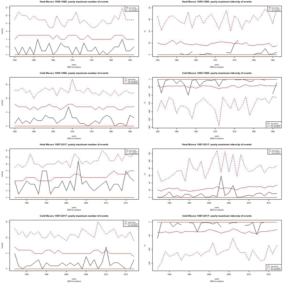
Figure 6. Yearly maximum number of events (left panels) and yearly maximum intensity of the events (right panels) for heat waves and cold waves in 1955-1986 (first two lines) and in 1987–2017 (last two lines). In all figures, the black lines are for the observations, the red lines correspond to the 90% Confidence Interval from the reconstructed trajectories and the dotted red line illustrates the maximum obtained from the reconstructed trajectories.

Changes in the Frequency of the Most Extreme Events

Definitions

With the consideration of four climate models to retrieve the trends and 500 simulations of the residuals, 2000 trajectories of the daily thermal indicator in France over the period 1955–2017 are produced. From such a large sample, it is possible to infer changes in the frequency of intense heat waves and cold waves between both periods (i.e., the calibration period 1955–1986 and the validation period 1987–2017). Based on the most extreme observed events as summarized in Table 2, intense cold waves will be defined as events with an intensity lower than −90 and very severe cold waves as events with an intensity lower than −95. Intense heat waves will be defined as events with an intensity higher than 55 and very severe events as events with an intensity higher than 60.

With these definitions, Table 4 compares the results in terms of number and frequency of these events between the periods 1955–1986 and 1987–2017. It shows that the frequency of occurrence of intense and very severe cold waves as defined in this study may have reduced by a factor of 3 between the periods 1955–1986 and 1987–2017, whilst that of intense and very severe heat waves may have increased by a factor of 4–5 on average.

TABLE 4

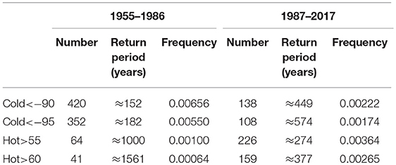
Table 4. Number and frequency (mean number per year) of intense and very severe heat and cold waves in period 1955–1986 and 1987–2017.

Sensitivity Tests

After this first application of the proposed methodology, different tests have been made to assess the importance of some modeling choices.

Firstly, the same procedure has been used with another set of four independent climate models, independency being defined as previously by the fact that they do not share the same model for any of the four components of the climate system. The new set comprises models BCC-CSM1.1, CanESM2, CCSM4, and EC-EARTH.

Then, for each set of four climate models, the non-parametric trends in mean and standard-deviation have been estimated with the same smoothing parameter as for the observations in period 1955–1986 (0.2), rather than looking for the optimal smoothing parameter for each model as has been previously done. This allows testing for the influence of the smoothing parameter in the derivation of the trends.

Table 5 summarizes validation results and changes in the frequency of intense and very severe events. The same weakness in the reproduction of the maximum number of hot events in the period 1987–2017 can be observed, whatever the climate models or the smoothing parameters. In parallel, a slight tendency of underestimating the intensity of the coldest events can also be noticed, with 3 observed years with an event of maximum intensity lower than the lower bound of the 90% confidence interval given by the simulations, whereas around 1.5 would be expected. One thus can note some asymmetry in the performances of the generation, with a small discrepancy for the maximum number of hot events per year and for the maximum intensity of cold events. Furthermore, the results show that for cold waves, the influence of the smoothing parameter to infer the trends is quite low, while the choice of the climate models seems to have a greater impact. The decrease in the frequency of intense and very severe cold events is smaller (factor of 2) with the second set of models than with the first one (factor of 3). For the most severe heat waves, the smoothing parameter seems to have some impact, at least with the first set of models (frequency 0.00044 with 0.2 and 0.00064 with the optimal smoothing parameter of each model), and again the change between the periods is slightly smaller with the second set of models (factor of around 3.5) than with the first one (factor of around 4–5).

TABLE 5

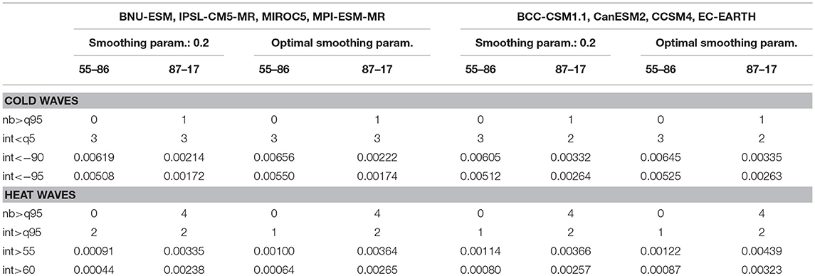
Table 5. Validation of the maximum number (nb) and maximum intensity (int) of heat and cold waves (number of years with higher numbers of events than the 90% Confidence Interval upper bound: nb > q95 and number of years with cold events with an intensity lower than the 90% CI lower bound: int < q5 or hot events with an intensity higher than the 90% CI upper bound: int > q95) and frequency of intense (int < −90 for cold waves, int > 55 for heat waves) and very severe events (int < −95 for cold waves and int > 60 for heat waves) in periods 1955–1986 and 1987–2017 according to different sensitivity tests.

Lastly, the number of generated trajectories of the residuals Z(t) has been tested. Figure 7 shows the evolution of the frequency of intense and very severe events as a function of the number of generations of Z(t) used to create the sample, for hot and cold events and for each set of four climate models. It shows that the frequencies stabilize from a number of around 500 generations in all cases, which means that from this number of simulations, the sensitivity to the stochastic generation can be neglected. Furthermore, the second set of models leads to smaller changes in the frequency of intense and very severe cold events (division by a factor of ~2 compared to around 3) as well as for the intense and very severe hot events, although in a lesser extent (multiplication by a factor of 4.5–5 compared to 5–5.5).

FIGURE 7

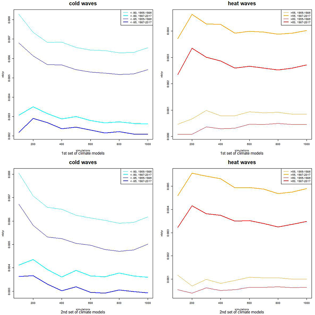
Figure 7. Evolution of the frequency of intense (intensity < −90, cyan) and very severe (intensity < −95, blue) cold events as a function of the number of stochastic simulated evolutions of the residuals for period 1955–1986 (thin lines) and 1987–2017 (bold lines) with the first set of four climate models (top left panel); evolution of the frequency of intense (intensity > 55, orange) and very severe (intensity > 60, red) hot events as a function of the number of stochastic simulated evolutions of the residuals for period 1955–1986 (thin lines) and 1987–2017 (bold lines) with the first set of four climate models (top right panel); bottom panels: same as top panels but for the second set of climate models.

Changes Between Periods 1955–1986 and 1987–2017

The previous tests have shown the importance of the choice of the climate models, and suggested that the choice of the smoothing parameter for the non-parametric trends may have an impact, thus justifying the identification of the optimal smoothing parameters. Moreover, it seems that the simulation of 500 different time series for the residuals is sufficient. Therefore, one way proposed here to better estimate the changes in the frequency of intense and very severe events between periods 1955–1986 and 1987–2017 is to use the full set of 23 model simulations together with 500 time series of the residuals. Then, for each model based trend couple (trend for the mean and for the standard deviation), 500 thermal indicator time series are built. From each of the 23 sets of 500 time series, a frequency of intense and very severe events for each period can be derived, which then allows estimating the changes between both periods. This thus produces a sample of 23 frequency changes (computed as the ratio between frequency in period 1987–2017 and in period 1955–1986), from which it is possible to obtain a mean change and a range of such changes, given by the minimum and the maximum over all climate models. The results are given in Table 6. They show that the frequency of intense and very severe cold waves has been reduced by a factor of 2 on average, with one model leading to a larger decrease (division by a factor of around 5) and another one projecting almost no change. Concerning intense and very severe heat waves, for a majority of models the frequency has been largely increased, by a factor of 4 on average, with one model even giving a factor of around 10.

TABLE 6

Table 6. Distribution of the frequency changes for intense and very severe heat and cold waves between periods 1955–1986 and 1987–2017 obtained with the 23 climate model simulations, expressed as the ratio between frequencies in each period (frequency in 1987–2017/frequency in 1955–1986).

The observations only give one trajectory, from which it is impossible to infer a frequency for events of such intensity, but the fact that the frequency of severe cold waves has decreased and the frequency of severe heat waves has increased is consistent with the observations. Furthermore, these findings are in line with previous studies which have estimated that human activities have increased of a factor around 4 the probability of an event like the 2003 heat wave compared to what it would have been without the recent warming (Stott et al., 2004; Coumou and Rahmstorf, 2012; Francis and Vavrus, 2012). The 2003 heat wave is close to what has been considered here as a very severe event (intensity 59.4 while very severe events are defined by an intensity higher or equal to 60). The quantification of the frequency change of extreme cold events seems to be more difficult and quantifications can hardly be found in the literature. In Europe, cold events are linked to anticyclonic blocking situations or by a flow of very cold Arctic air from the polar region. But most climate models tend to overestimate the meridional pressure gradient, implying too moist and mild conditions and fewer blocking events (van Ulden and van Oldenborgh, 2006; Brands et al., 2013). Thus, the change evaluated here is difficult to validate against other studies.

Application to the Production of Possible 1981–2040 Trajectories

The previously described and tested approach is then used to build a large sample of possible thermal indicator evolutions in the next decades. To do so, the generator is first calibrated by using the observations between 1951 and 2010. As a matter of fact, the estimates of trends are more robust when made from a larger sample. The stochastic SFHAR model is fitted to the estimated residuals and 500 equivalent trajectories are simulated. Then, the non-parametric trends in mean and standard deviation in the period 1981–2040 are derived for each simulation of the 23 climate models and bias adjusted to the observed trends in the period 1981–2010 (Figure 8). The combination of these sets of trends with the observed seasonality and the 500 simulated trajectories of residuals allows the construction of a large set of 23 times 500 trajectories covering the period 1981–2040, from which, in the same way as previously, the changes in frequency of intense and very severe hot and cold events can be studied. The results are given in Table 7 and they indicate a larger decrease in the frequency of very cold events than had been experienced in 1987–2017 compared to 1955–1986. In the period 2011–2040, the considered climate models project a reduction by a factor of 5 on average in the frequency of intense and very severe cold events compared to period 1981–2010, whereas this reduction was a factor of 2 between the previously considered historical periods. On the other hand, the frequency of extreme hot events is projected to increase further, but here in a lesser extent than what had been estimated for the historical periods; the models project on average a doubling of the frequency of 1981–2010 in the coming 2011–2040 period, compared to a factor of 4 increase between 1955–1986, and 1987–2017. The previous mean values correspond now to the maxima instead.

FIGURE 8

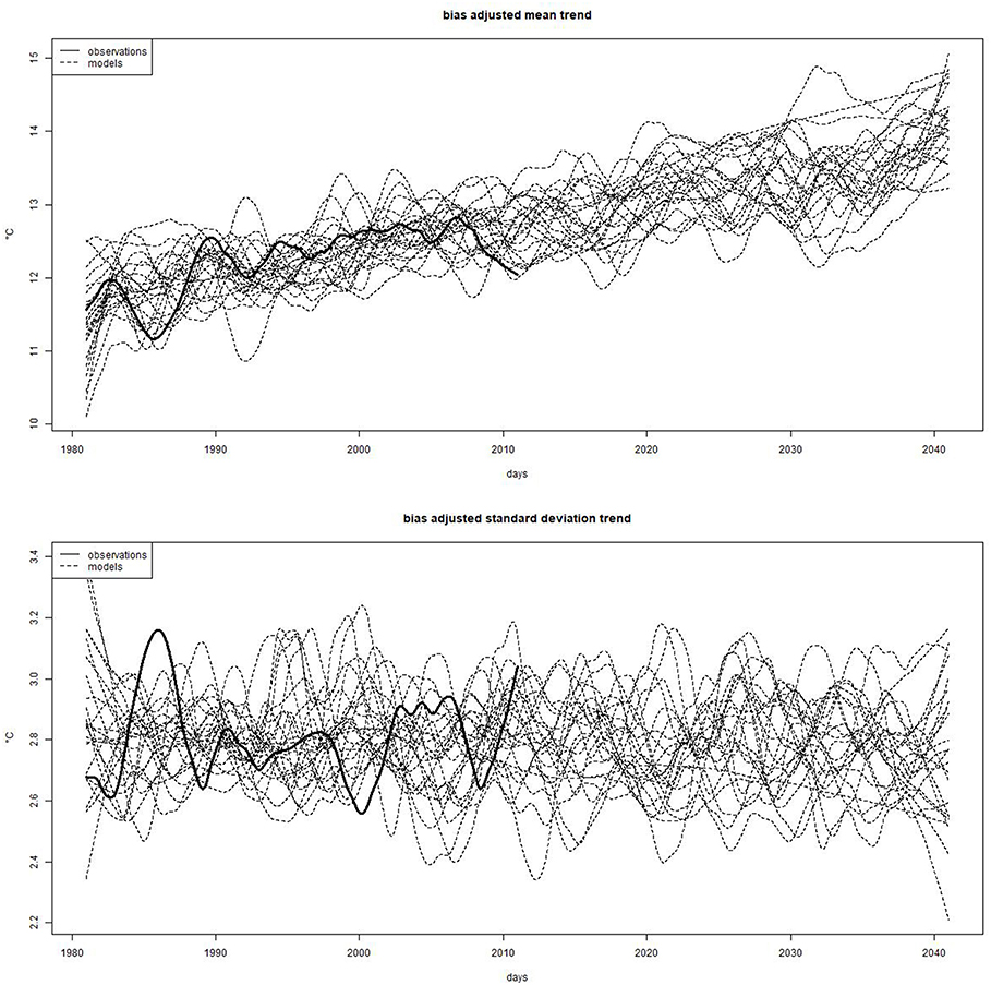
Figure 8. Bias-adjusted trends in mean (top panel) and standard deviation (bottom panel) obtained from the 23 climate model simulations for the period 1981–2040 (dotted lines) with the observed trends in period 1981–2010 superimposed (black line).

TABLE 7

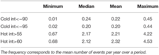
Table 7. Distribution of the frequency changes for intense and very severe heat and cold waves between periods 1981–2010 and 2011–2040 obtained with the 23 climate model simulations, expressed as the ratio between frequencies in each period (frequency in 2011–2040/frequency in 1981–2010).

Discussion and Perspectives

In this study, a methodology has been proposed and tested to build a very large sample of a temperature based indicator over the recent past and the next decades. The approach is based on the decomposition of the time series into deterministic parts (seasonality and trends), and a stochastic residual part. Previous work had shown that this residual part can be considered as stationary with an annual periodicity, and a stochastic model has been put in place to simulate it. The construction of the evolution of the indicator over the recent past and the next decades is then obtained by combining observed seasonality with climate model derived trends and a large sample of trajectories for the residual part.

The proposed approach has first been checked in a cross-validation setting. It has been shown to be reasonable, although a tendency to slightly underestimate the maximum number of warm events per year and slightly underestimate the maximum cold event intensity has been shown. Then, sensitivity tests have highlighted the importance of climate model choice and identified a number of the 500 trajectories of the residuals as the minimum required to stabilize the estimations of events frequencies and frequency changes.

Based on these outcomes, an evaluation of the changes in frequency of past extreme hot and cold events has been proposed, based on a set of 23 climate model simulations. Concerning historical changes between the periods 1955–1986 and 1987–2017, an average reduction by a factor of 2 of the frequency of intense and very severe cold events has been found, while the frequency change for the intense and very severe hot events is estimated as having been increased by a factor of 4 on average. These findings are consistent both qualitatively with the observations and quantitatively with previous studies in the literature. Then, the changes in the coming decades (period 2011–2040) compared to the current climate (period 1981–2010) are shown to go in the same direction, but with a larger decrease in the frequency of extreme cold events (reduction by a factor of 5 on average) and a smaller increase in the frequency of extreme hot events (increase by a factor of 2 on average).

These results have to be considered as a first step and the approach could undergo further analyses. First, the role of the choice of the calibration period should be investigated further. Secondly, a larger set of climate model simulations could be considered, including different runs for each model, as it could lead to a larger sample of possible combinations of long term climate variability and change. A clustering step may then help identifying possible evolutions shared by groups of simulations. Furthermore, this approach could be compared to other techniques used in the literature to estimate past or future changes in the frequency of extreme events.

The proposed approach is used here to estimate possible changes in the frequency of extreme events in relation to electricity demand through the use of a dedicated thermal indicator. The same setting may allow for the consideration of decadal predictions rather than climate projections when available. A further step will be to generate consistent sets of such trajectories for the different climate variables influencing electricity demand and generation (e.g., precipitation, wind, and radiation). Such a generator based on hidden Markov models has recently been proposed (Touron, 2019) and its use in a climate change context will be studied further.

Data Availability

Publicly available datasets were analyzed in this study. This data can be found here: https://www.ecad.eu/download/ensembles/download.php.

Author Contributions

SP proposed the approach based on previous developments made in collaboration with colleagues and academic scientists, as well as the outline of the validation tests and the applications. She wrote the codes in R devoted to the calculations discussed in the paper and wrote the paper.

Conflict of Interest Statement

The author declares that the research was conducted in the absence of any commercial or financial relationships that could be construed as a potential conflict of interest.

Acknowledgments

The author acknowledges the E-OBS dataset from the EU-FP6 project ENSEMBLES (http://ensembles-eu.metoffice.com) and the data providers in the ECA&D project (http://www.ecad.eu).

Special thanks to S. Denvil (IPSL) for providing the CMIP5 simulations and to Paul-Antoine Michelangeli (EDF/R&D) for preparing and managing the EDF climate model results database.

References

Añel, J. A. (2015). On the importance of weather and climate change for our present and future energy needs, edited by Troccoli, Dubus and Ellen Haupt. Contemp. Phys. 56, 206–208. doi: 10.1080/00107514.2015.1006251

CrossRef Full Text | Google Scholar

Añel, J. A., Fernández-González, M., Labandeira, X., López-Otero, X., and de la Torre, L. (2017). Impact of cold waves and heat waves on the energy production sector. Atmosphere. 8:209. doi: 10.3390/atmos8110209

CrossRef Full Text | Google Scholar

Auffhammer, M., Baylis, P., and Hausman, C. H. (2017). Climate change is projected to have severe impacts on the frequency and intensity of peak electricity demand across the United States. Proc. Natl. Acad. Sci. U.S.A. 114, 1886–1891. doi: 10.1073/pnas.1613193114

PubMed Abstract | CrossRef Full Text | Google Scholar

Benth, E. F., and Saltyte Benth, J. (2011). Weather derivatives and stochastic modelling of temperature. Int. J. Stoch. Anal. 2011:576791. doi: 10.1155/2011/576791

CrossRef Full Text | Google Scholar

Bessec, M., and Fouquau, J. (2008). The non-linear link between electricity consumption and temperature in Europe: a threshold panel approach. Energy Econ. 30, 2705–2721. doi: 10.1016/j.eneco.2008.02.003

CrossRef Full Text | Google Scholar

Boé, J. (2018). Interdependency in multimodel climate projections: component replication and result similarity. Geophys. Res. Lett. 45, 2771–2779. doi: 10.1002/2017GL076829

CrossRef Full Text | Google Scholar

Bossmann, T., and Staffell, I. (2015). The shape of future electricity demand: exploring load curves in 2050s Germany and Britain. Energy 90, 1317–1333. doi: 10.1016/j.energy.2015.06.082

CrossRef Full Text | Google Scholar

Brands, S., Herrera, S., Hernández, J., and Gutiérrez, J. M. (2013). How well do CMIP5 earth system models simulate present climate conditions in Europe and Africa? A performance comparison for the downscaling community. Clim. Dyn. 41, 803–817. doi: 10.1007/s00382-013-1742-8

CrossRef Full Text | Google Scholar

Bruhns, A., Deurveilher, G., and Roy, J. S. (2005). “A non-linear regression model for mid-term load forecasting and improvements in seasonality,” in 15th PSCC Session 17, Paper 2 (Liege).

Google Scholar

Campbell, S. D., and Diebold, F. X. (2005). Weather forecasting for weather derivatives. J. Am. Stat. Assoc. 100, 6–16. doi: 10.1198/016214504000001051

CrossRef Full Text | Google Scholar

Chandler, R. E. (2005). On the use of generalized linear models for interpreting climate variability. Environmetrics 16, 699–715. doi: 10.1002/env.731

CrossRef Full Text | Google Scholar

Coumou, D., and Rahmstorf, S. (2012). A decade of weather extremes. Nat. Clim. Chang. 2, 491–496. doi: 10.1038/nclimate1452

CrossRef Full Text | Google Scholar

Dacunha-Castelle, D., Hoang, T. T. H., and Parey, S. (2015). Modeling of air temperatures: preprocessing and trends, reduced stationary process, extremes, simulation. J. Soc. Franç. Stat. 156, 138–168. Available online at: http://www.sfds.asso.fr/journal

Google Scholar

Francis, J. A., and Vavrus, S. J. (2012). Evidence linking Arctic amplification to extreme weather in midlatitudes. Geophys. Res. Lett. 39:L06801. doi: 10.1029/2012GL051000

CrossRef Full Text | Google Scholar

Furrer, E. M., and Katz, R. W. (2007). Generalized linear modeling approach to stochastic weather generators. Clim. Res. 34, 129–144. doi: 10.3354/cr034129

CrossRef Full Text | Google Scholar

Glenis, V., Pinamonti, V., Hall, J., and Kilsby, C. (2015). A transient stochastic weather generator incorporating climate model uncertainty. Adv. Water Resour. 85, 14–26. doi: 10.1016/j.advwatres.2015.08.002

CrossRef Full Text | Google Scholar

Godfarb, D., and Idnani, A. (1983). A numerically stable dual method for solving strictly convex quadratic programs. Math. Program. 27, 1–33. doi: 10.1007/BF02591962

CrossRef Full Text | Google Scholar

Golfarb, D., and Idnani, A. (1982). “Dual and primal-dual methods for solving strictly convex quadratic programs,” in Numerical Analysis, ed J. P. Hennart (Berlin: Springer-Verlag), 226–239.

Haylock, M. R., Hofstra, N., Klein Tank, A. M. G., Klok, E. J., Jones, P. D., and New, M. (2008). A European daily high-resolution gridded dataset of surface temperature and precipitation. J. Geophys. Res. 113:D20119. doi: 10.1029/2008JD010201

CrossRef Full Text | Google Scholar

Hoang, T. T. H. (2010). Modélisation de séries chronologiques non stationnaires, non linéaires: application à la définition des tendances sur la moyenne, la variabilité et les extrêmes de la température de l'air en Europe. Ph.D. thesis, University of Paris 11, Orsay, France.

IPCC (2013). “Climate change 2013: the physical science basis,” in Contribution of Working Group I to the Fifth Assessment Report of the Intergovernmental Panel on Climate Change, eds T. F. Stocker, D. Qin, G.-K. Plattner, M. Tignor, S. K. Allen, J. Boschung, et al. (Cambridge; New York, NY: Cambridge University Press), 1535.

Google Scholar

Luo, D., Yao, Y., and Feldstein, S. B. (2014), Regime transition of the North Atlantic oscillation the extreme cold event over europe in January–February 2012. Mon. Weather Rev. 142, 4735–4757. doi: 10.1175/MWR-D-13-00234.1

CrossRef Full Text | Google Scholar

Marron, J. S. (1987). Partitioned cross-validation. Econ. Rev. 6, 271–284. doi: 10.1080/07474938708800136

CrossRef Full Text | Google Scholar

Massey, N., Jones, R., Otto, F. E. L., Aina, T., Wilson, S., Murphy, J. M., et al. (2014). weather@home—development and validation of a very large ensemble modelling system for probabilistic event attribution. Q. J. R. Meteorol. Soc. 141, 1528–1545. doi: 10.1002/qj.2455

CrossRef Full Text | Google Scholar

McFarland, J., Zhou, Y., Clarke, L., Sullivan, P., Colman, J., Jaglom, W. S., et al. (2015). Impacts of rising air temperatures and emissions mitigation on electricity demand and supply in the United States: a multi-model comparison. Clim. Change 131:111–125. doi: 10.1007/s10584-015-1380-8

CrossRef Full Text | Google Scholar

Mraoua, M., and Bari, D. (2007). Temperature stochastic modelling and weather derivatives pricing: empirical study with Moroccan data. Afr. Stat. 2, 22–43. doi: 10.4314/afst.v2i1.46865

CrossRef Full Text

Nelder, J., and Mead, R. (1965). A simplex algorithm for function minimization. Comput. J. 7, 308–313. doi: 10.1093/comjnl/7.4.308

CrossRef Full Text | Google Scholar

Parey, S., Hoang, T. T. H., and Dacunha-Castelle, D. (2014). Validation of a stochastic temperature generator focusing on extremes and an example of use for climate change. Clim. Res. 59, 61–75. doi: 10.3354/cr01201

CrossRef Full Text | Google Scholar

Richardson, C. W. (1981). Stochastic simulation of daily precipitation, temperature, and solar radiation. Water Resour. Res. 17, 182–190. doi: 10.1029/WR017i001p00182

CrossRef Full Text | Google Scholar

RTE (2012). La Vague de Froid de Février 2012. Paris: Direction Économie Prospective et Transparence. Available online at: www.rte-france.com

Santamouris, M., Cartalis, C., Synnefa, A., and Kolokotsa, D. (2015). On the impact of urban heat island and global warming on the powerdemand and electricity consumption of buildings—a review. Energy Build. 98, 119–124. doi: 10.1016/j.enbuild.2014.09.052

CrossRef Full Text | Google Scholar

Smith, K., Strong, C., and Rassoul-Agha, F. (2017). A new method for generating stochastic simulations of daily air temperature for use in weather generators. J. Appl. Meteorol. Climatol. 56, 953–963. doi: 10.1175/JAMC-D-16-0122.1

CrossRef Full Text | Google Scholar

Stone, C. J. (1977). Consistent nonparametric regression. Ann. Stat. 5, 595–620. doi: 10.1214/aos/1176343886

CrossRef Full Text | Google Scholar

Stott, P. A., Stone, D. A., and Allen, M. R. (2004). Human contribution to the European heat wave of 2003. Nature 432, 610–614. doi: 10.1038/nature03089

CrossRef Full Text | Google Scholar

Touron, A. (2019). Consistency of the maximum likelihood estimator in seasonal hidden Markov models. Stat. Comput. 1–21. doi: 10.1007/s11222-019-09854-4

CrossRef Full Text | Google Scholar

Troccoli, A., Dubus, L., and Haupt, S. E. (2014). Weather Matters for Energy. New York, NY: Springer.

Google Scholar

van Ulden, A. P., and van Oldenborgh, G. J. (2006). Large scale atmospheric circulation biases and changes in global climate model simulations and their importance for climate change in Central Europe. Atm. Chem. Phys. 6, 863–881. doi: 10.5194/acp-6-863-2006

CrossRef Full Text | Google Scholar