Simulation of Long-Term Changes of the Equilibrium Line Altitude in the Central Chilean Andes Mountains Derived From Atmospheric Variables During the 1958–2018 Period

Introduction

The Chilean Andes Cordillera is the world's longest continental mountain range, which extends in a north-south direction from about 55°S northward, crossing all the western side of South America. The distinct climatic conditions (mainly precipitation and air temperature) and the differences in physiographic characteristics of the territory such as terrain slope, drainage basin area and geographical orientation, feature the ice-mass fluctuations of the thousands of glaciers that dissect the Andes mountain valleys (Barcaza et al., 2017; Braun et al., 2019).

The climatic characteristics of central Chile (located between ~30 and 38°S) are defined by the permanent influence of the South Pacific High-Pressure Center and the seasonal north-south displacement of the westerly regime that steers frontal depressions toward central Chile mostly during the winter (Carrasco et al., 2005). Along with these meteorological factors, the climate is also defined by the regional topography characterized by a low-altitude coastal range, an intermediate depression (where Santiago de Chile is located) and the high Andes mountains to the East (Figure 1). All these factors result in an overall air temperature decrease from North to South and a West-East gradient with increasing mean-annual air temperature from the coastal zone to the intermediate depression and decreasing from this zone to the Andes mountains (Figure 2A).

FIGURE 1

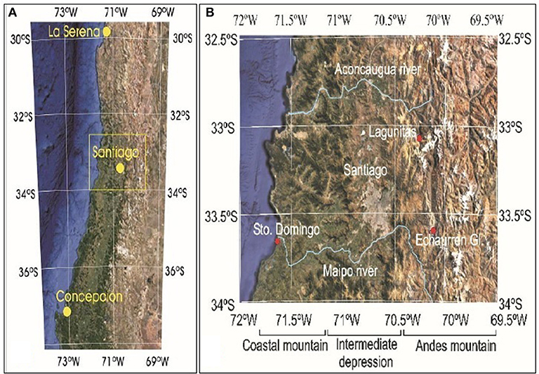
Figure 1. Location map of central Chile (A). Yellow box is the zoom displayed in (B).

FIGURE 2

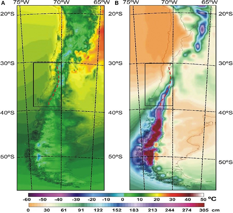
Figure 2. Near surface annual average air temperature (2 m) and annual average precipitation (1979–2010 period) constructed using the NASA-MERRA 2 reanalysis data from the ClimateReanalyzer.org of the Climate Change Institute, University of Maine, United States.

The spatial distribution of the annual precipitation shows a southward increment and an increase with terrain elevation (Figure 2B) due to the mountain effect on the passing frontal systems (Garreaud, 2009; Viale and Garreaud, 2015) and atmospheric rivers (Viale et al., 2018), which can enhance precipitation by a factor of 2–3 in central Chile (Falvey and Garreaud, 2007). Every year snow precipitation seasonally covers the high elevation areas of the region of study, where the air temperature falls below the freezing level (Mernild et al., 2016; Stehr and Aguayo, 2017). Furthermore, the region displays significant interannual climate variability, which is mainly associated with El Niño Southern Oscillation (ENSO) and the Antarctic Annular Mode (AAM, Quintana and Aceituno, 2012). While the interdecadal fluctuations can be related to the PDO (Montecinos and Aceituno, 2003), the observed secular long-term trends have been mainly attributed to climate change (Christidis et al., 2010; Boisier et al., 2016, 2018).

Winter snow accumulation and glaciers in the Andes are the primary source for streamflow at both, the Chilean and Argentinian sides of the mountains (e.g., Ayala et al., 2016). Their freshwater contribution to the main rivers of the semiarid region are larger during summer months (Ragettli and Pellicciotti, 2012) and during drought years (Peña and Nazarala, 1987; Favier et al., 2009; Migliavacca et al., 2015). Unfortunately, studies of snow cover, snow depth, snowfall, and snow water equivalent (SWE) are still scarce in the region mainly related to the lack of long and well distributed data. Proxy information like Equilibrium Line Altitude (ELA, Cogley et al., 2011), snowpack (Masiokas et al., 2006, 2010), and satellite data (Foster et al., 2009) have been used to assess the ice-snow changes in South America. In particular, measurements of the ELA require field observations in remote mountains areas which are scarce and infrequent. Then, estimations of ELA (named here ELA_model) derived from the annual average of the 0°C isotherm altitude (ZIA) and the annual precipitation accumulated in mountains areas (Condom, 2002; Carrasco et al., 2005, 2008; Condom et al., 2007) are a useful source of information to assess interannual and interdecadal variability of snow-ice cover in mountain areas. In this regard, the present study aims to update the Carrasco et al. (2005) analysis of variability and trends of the central Chilean Andes ELA by using radiosonde and new available precipitation datasets until 2018.

Climate and Environmental Changes

The mean annual near-surface air temperature and annual precipitation data from the Environmental Change Model (ECM), based on the NASA MERRA-2 reanalysis data during the 1979–2010 period, are presented in Figures 2A,B, respectively. According to Figures 2A,B, constructed using the ClimateReanalyzer interface (climatereanalyzer.org/clim/ecm/), there is important spatial variability in temperature and precipitation data in the region of study (black rectangle). For example, a difference of about −4°C (−10°C) in the minimum (maximum) monthly mean air temperature is observed between the ski resort Farellones (33.35°S, 70.30°W) placed at 2570 m a.s.l., and weather stations located in the intermediate depression (located at ~500 m a.s.l.).

Additional information derived from radiosonde data recorded at Santo Domingo station (~150 km to the West of the Andes mountains), shows that the monthly air temperature (using the 2000–2017 period) in the free-atmosphere ranges from 8.4 ± 1.0°C and −0.9 ± 1.5°C at 700 hPa (~3110 ± 19 m); to −10.3 ± 1.0°C, and −18.5 ± 1.2°C at 500 hPa (~5749 ± 52 m), in January and July, respectively. In addition, the annual average (1981–2016) of the zero-isotherm altitude (ZIA) is 3684.2 ± 95.9 m, with a minimum of 3039.5 ± 254.0 m in July and an altitude of 4244.3 ± 156.9 m in March (end of the austral summer season). That West-East altitudinal gradient of the air temperature reveals that the Andes mountains, characterized by a mean elevation that surpasses 4000 m a.s.l., present favorable atmospheric conditions for the presence of glaciers and snow seasonal accumulation during winter months in central Chile.

Over the last decades, the intermediate depression and the Andes mountain range of central Chile have experienced sustained increases in temperature, with observed trends of about 0.25°C/decade (Burger et al., 2018), warming that also prevails in the Argentine side of the Andes (Falvey and Garreaud, 2009). Despite that, a cooling of −0.1 to −0.3°C per decade in the coastal zone was reported (Hartmann et al., 2013; Vuille et al., 2015), which according to a recent study has already ended (Burger et al., 2018); the linear trend of the surface air temperature in central Chile shows an overall warming of 0.2–1.0°C during the 1901–2012 period, as derived from HadCRUT4, MLOST, and GISS data sets (Hartmann et al., 2013).

On the other hand, the spatial distribution of the mean annual precipitation shows an increase from North to South and from the intermediate depression to the high Andes mountains. Along the central high Andes mountains, the annual precipitation increases from around 300 mm at ~30°S to 2280 mm at ~38°S. The precipitation time series show strong seasonal behavior with dry conditions in summer (December–February) and more than 90% of the total annual precipitation falling during the wet season, from May to September (Falvey and Garreaud, 2007).

Hartmann et al. (2013) revealed an overall negative trend in precipitation in central Chile that ranges from −2.5 to −50 mm yr⁻¹ per decade for the 1901–2010 period, depending on the database used [Climate Research Unit (CRU), Global Historical Climate Network (GHCN) or Global Precipitation Climatology Centre (GPCC)]. La Serena, Santiago and Concepción meteorological stations, located in the northern, central and southern part of the studied region, have precipitation records available for the 1900–2018 period. Their respective linear trends indicate a decrease in precipitation of about −5.6 ± 1.0, −6.8 ± 0.8, and −33.0 ± 1.4 mm/decade, all statistically significant (p < 0.05). More recently, a period of consecutive dry years has occurred in central Chile from 2010 to 2018. Due to the extraordinary character and uniqueness of the significant precipitation decline in central-southern Chile during 2010–2018, the event has been named as megadrought (Garreaud et al., 2017).

Cryospheric Review in Central Chile

The ELA is the spatially averaged altitude of the equilibrium line on the surface of a glacier where at a given moment the climate surface mass balance is zero (Cogley et al., 2011), i.e., the ELA separates the accumulation from the ablation zone. It can be obtained from field observations and aerial and satellite imagery for the end of the summer season (Chinn, 1999; Rabatel et al., 2005), when snowline observations are used as a proxy of the ELA in the southern Andes. Two estimations of ELA (ELA_model) were derived in central Chile in the last decade: Carrasco et al. (2005) estimated the ELA_model in the western side of the central Chilean Andes between ~30 and 38°S, and later Carrasco et al. (2008) obtained the ELA_model for the region between ~18 and 55°S. In central Chile the results of the ELA_model behavior revealed an increase in 102 ± 6 m for the 1958–2006 period, which was non-statistically significant at the 95% level. The climate shift of 1976/77 (Giese et al., 2002) was also clearly revealed by the time series, with negative (cooling) trends before 1976 and a positive (warming) trend after 1977. Moreover, analysis of the mean ZIA indicates predominantly warmer conditions during the 1977–2006 period (statistically significant at the 95% level, p < 0.05), compared to the 1958–76 period. The ELA_model increment after the climate shift was 111 ± 9 m in the central region for the 1978–2006 period, which is statistically significant (p < 0.05).

Regarding snowpack, a direct analysis was carried out by Masiokas et al. (2006) using snow course data from both sides of the central Andes in Chile and Argentina (30–37°S). The regional maximum of snow water equivalent (MSWE) time series (1951–2005) were approximately normally distributed and showed a marked interannual variability and a positive linear trend (+3.95% decade⁻¹), although non-significant. They found that the interannual variability correlates with ENSO during the austral winter months (see also Cortés and Margulis, 2017). A later study by Masiokas et al. (2010) used the snowpack and the mean annual river flows to analyse their inter and multidecadal variations. Analysis of the regional streamflow composite (1906–2007) showed an insignificant negative trend, but a significant regime shift in 1945, when the mean levels dropped 31%, and in 1977 when they increased 28%. The fluctuations of decadal streamflow phases were also observed in the regional snowpack series (1951–2008), but the latter has not significant regime shifts. However, the snowpack composite series revealed large interannual variability and a slight positive trend, which are concurrent with the positive and negative phases of the PDO.

An analysis of the seasonal snow cover and snow mass variability in South America was conducted by Foster et al. (2009), by using SMMR (Scanning Multichannel Microwave Radiometer) and SSM/I (Special Sensor Microwave Imagers) passive microwave data from 1979 to 2006. Foster et al. (2009) found a decline in the average snow cover (May-September) and a slightly upward trend for snow mass during the 1979–2006 period, but they were not statistically significant. Still, uncertainties can affect these results (Foster et al., 2009). On the other hand, increases in central Chile glacier melt have been suggested from mountain basin (28–47°S) runoff analyses, which revealed slightly positive linear trends (not statistically significant) for most of the studied stations (13) during the 1950–2007 period (Casassa et al., 2009).

In a recent study, Saavedra et al. (2018) assessed snow persistence (yearly duration of the snow cover) in the region extended from 8° to 36°S, during 2000 and 2016, using the Moderate Resolution Imaging Spectroradiometer (MODIS) data. They found a significant loss of snow cover (2–5 fewer days of snow year⁻¹) between the 29 and 36°S, which was more pronounced (62% of the area with significant trends) on the eastern side of the Andes. They also found a significant increase in the elevation of the snowline of 10–30 m year⁻¹ south of 29–30°S. Their analyses indicated that these changes are correlated with decreasing precipitation and increasing air temperature, and that the magnitudes of the correlations vary with latitude and elevation. Moreover, they found that ENSO has a good correlation with snow persistence conditions north of 31°S, whereas the SAM has larger influence south of 31°S.

Also, Malmros et al. (2018) found an average decrease of −13 ± 4%, −7.4 ± 2%, and −43 ± 20 days in snow cover extend (SCE), snow albedo (SAL) and snow cover duration (SCD), respectively, during the 2000–2016 period in the central Andes of Chile and Argentina using MODIS daily snow product (MOD10A1 C6). They also found significant correlation between Multivariate El Niño (MEI) and the SCE and the SAL with a 1-month time-lag. Moreover, during the study period, largest SCD changes occurred at elevations below 4,500 m a.s.l. on the eastern side and below 3,500 m a.s.l. on the western side of the Andes.

In response to the environmental changes, glaciers have been retreating and thinning in the central Chilean Andes mountains (Casassa et al., 2007), with area reductions between −0.5%/decade and −2.4%/decade in the period 1955–2001 (Rivera et al., 2002; Pellicciotti et al., 2014). Frontal glacier retreats between −9 and −50 m/year have been reported for central Chile and Argentina, and negative surface mass balance (SMB) between −0.56 and −0.76 m/year have been reported for central Chilean and Argentinean glaciers (Le Quesne et al., 2009, see also Malmros et al., 2016). Analyses of SMB obtained from Piloto Glacier (Argentina) and Echaurren Norte Glacier (Chile), respectively, showed a cumulative mass balance loss of −10.50 m w.e. for the 1979–2003 period (Leiva et al., 2007), and of −40.64 ± 5.19 m w.e. during the 1955–2015 period (Farias-Barahona et al., 2019).

Data and Method

Zero Isotherm Altitude

Daily upper-level meteorological observations at 12 UTC from three radiosonde stations in Chile have been used in this study: Antofagasta (23°26' S, 70°26'W; 135 m a.s.l.), Quintero (32°47' S,71°33'W; 8 m a.s.l.), and Puerto Montt (41°26' S, 73°07' W; 81 m a.s.l.) stations. In October 1999, the areological station located at Quintero was moved ~100 km southward to its current location at Santo Domingo (33°38' S, 71°18' W, 77 m a.s.l.). To filter out the discontinuity given by the displacement of Quintero station, an adjustment was introduced and corrected time series for 1958–2018 were provided for Quintero/Santo Domingo (QSD) station. The adjustment consisted in determining correction factors of the air temperature time series and geopotential heights at 850, 700 and 500 hPa levels; by obtaining the average difference of each variable between 1980–1998 and 2000–2017 periods. Then, these differences were added to adjust the annual mean values from 1999 onward. The three areological stations were used to determine a latitudinal profile of the ZIA for central Chile, updating the Carrasco et al. (2005) work.

Monthly and annual tropospheric air temperature measured at the QSD station at different altitudes (850, 700, and 500 hPa) within 1958–2018 were used for yearly, decadal and long-term analyses (Figure 3). Cumulative Sum Charts (CUSUM) and Bootstrapping methods (Taylor, 2000; Khan et al., 2014) were used to detect abrupt changes in the annual temperature data. The CUSUM is the cumulative sums of the deviations from the average for individual temperature data, whose end-sum should be zero. The bootstrapping method determines the confidence level by using an estimator of the magnitude of the temperature times series change, which was applied on standardized anomalies. Based on those methods and if the climate data are homogenous, the significant changes in observed data can be associated to variations in weather and climate.

FIGURE 3

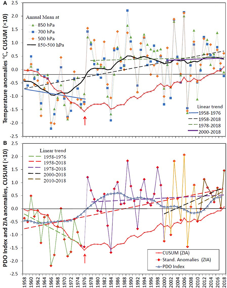
Figure 3. (A) Standardized anomalies of the air temperature at 850, 700, and 500 hPa from the Quintero/Santo Domingo areological station. Red curve is the cumulative sum of the mean anomalies. The red arrow indicates the significant climate change occurred in 1976/77. Black dashed line is the linear regression for the 1958–2017 period, blue line for the 1958–1976 period, green dashed line is for 1978–2018 period and violet line is for 2000–2018 period. The black curve is the smoothed temperature at 850-500 hPa time series, obtained after applying Equation 4. (B) Annual standardized anomalies of the ZIA (red squares), red dashed line is the linear regression over the 1958–2018 period. Green, violet, black, and brown dashed lines are the linear trends for the 1958–1976, 1977–2018, 2000–2018, and 2010–2018 periods, respectively. The blue line (with triangles) is the smoothed PDO time series, obtained after applying Equation 4.

On the other hand, the monthly averages of the vertical lapse rate derived from the temperature gradient between the 850 and 700 hPa, or the 700 and 500 hPa, were used to calculate the ZIA for each areological location. Then, the annual long-term means and standard errors of the ZIA at each station were calculated to obtain a polynomial expression (Equation 1) which represents the ZIA latitudinal profile (ZIA_lat) along the western slope of the Andes mountains. The latitudinal standard error at the 95% confidence level was determined by using the standard deviation of the monthly data.

$\begin{array}{ll}ZI{A}_{lat}=0.287\times L^3-33.322\times L^2+1101.6\times L-6548.7& (1)\end{array}$

with R² = 1; where L is the latitude in degrees south (L > 0), valid from 23 to 43°S. That expression provides the mean (and standard error) of the latitudinal altitude of the zero isotherm (ZIA_lat), based on the 1980–2010 period.

Latitudinal and Long-Term Time Series Precipitation

Most of the weather stations within the studied region are distributed in the coastal and intermediate depression with only a few stations placed in mountain areas located in the downstream outlet of the main catchments. Therefore, mountain precipitation needs to be estimated from existing rain-gauge, satellite, and model databases. A north-south distribution of the long-term annual-mean precipitation data was used in this study to obtain a latitudinal profile using all precipitation datasets (P_lat). To do that, the best polynomial expression which fits the annual-mean precipitation against the latitude data was selected:

$\begin{array}{ll}{P}_{lat}=c_1\times L^3+c_2\times L^2+c_3\times L+c_4& (2)\end{array}$

Where L is the latitude in degrees, that ranges from 30° to 38°S, and the coefficients (c_i) are determined by the polynomial relationship (depends on the database used). A latitudinal gradient of the annual-mean precipitation at the Andes was calculated by Carrasco et al. (2005), who used precipitation data from rain-gauges located at different altitudes for the 1961-1990 period (average of normalized precipitation), and a vertical gradient of precipitation to obtain the annual-mean precipitation above the 2,500 m.a.s.l within a latitudinal band of ±0.5°. The resulting mountain precipitation values were around 2–3 time higher than those obtained at the valley stations (Carrasco et al., 2005). These amounts are above the “correction ratio” factor of ~2 introduced by Adam et al. (2006) for correcting precipitation increment due to the orographic effect. Viale and Garreaud (2015) used rain-gauge and satellite data to determine the “enhancement rates” of 10 years-long (2002–2011) precipitation time series between the valley and the high elevations within a wide latitudinal band (30°-55°S). They found that the enhancement rate in central Chile corresponds to 1.92 for 33°-34°S, 2.20 for 34°-35°S, 2.26 for 35°-36°S, 1.82 for 36°-37°S, and 1.75 for 37°-38°S. Those values were also used in this study for calculating latitudinal profiles of precipitation at high elevations.

Additionally, the precipitation datasets provided by the CAMELS-CL (Catchment Attributes and MEteorology for Large sample Studies—Chile) (Alvarez-Garreton et al., 2018) were also included for constructing additional latitudinal profiles and long-term series of precipitation in the central Andes mountains (see the diagram in Figure 4). Four different gridded precipitation products were used, which are described in Table 1: (1) the CR2Met dataset (P-CR2), which is partly based on ERA-Interim reanalysis, (2) the Climate Hazard Group InfraRed Precipitation with Station data version 2 (P-CHIRPS, Funk et al., 2015), (3) the Multi-Source Weighed-Ensemble Precipitation data version 1.1 (P-MSWEP, Beck et al., 2017), and (4) the Tropical Rainfall Measuring Mission Multi-Satellite Precipitation Analysis (P-TMPA). Therefore, four additional latitudinal profiles were constructed for precipitation at high elevation using the P-CR2, P-CHIRPS and P-MSWEP for the 1981-2010 period, and the P-TMPA for the 1998–2010 period. To represent the changes of precipitation with latitude, polynomial functions similar to Equation 2, were adjusted to every precipitation dataset (Figures 4, 5).

FIGURE 4

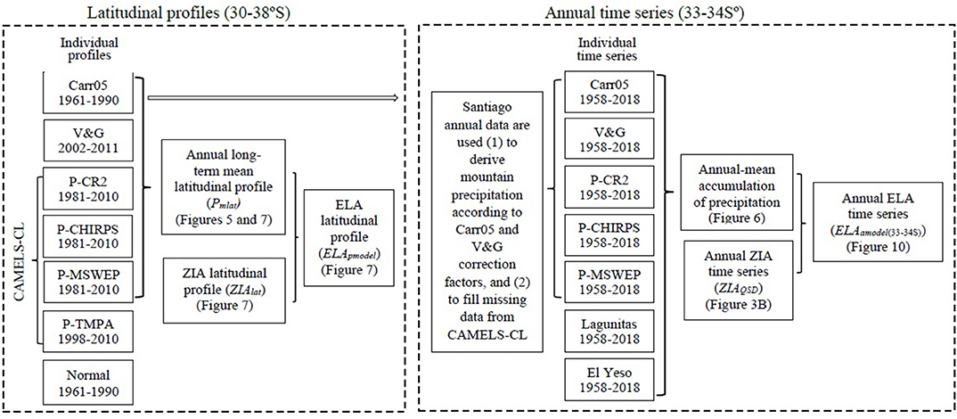
Figure 4. Flow chart of the datasets used to reconstruct the ELA_pmodel and ELA_{amodel(33−34S)}.

TABLE 1

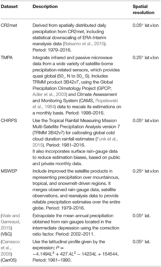
Table 1. Description of the precipitation datasets, the first 4 gathered from CAMELS-Cl (Alvarez-Garreton et al., 2018).

FIGURE 5

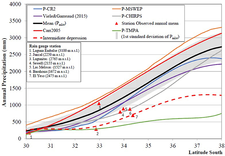
Figure 5. Latitudinal profiles of the mean annual Precipitation constructed from different datasets (Table 1). The red triangles are the mean annual precipitation observed at some mountain meteorological stations. Dashed red curve is the smooth latitudinal behavior of the mean annual precipitation in the intermediate depression.

The significant differences among the profiles (Figure 5) are related to the lack of well-distributed precipitation data in the mountainous areas, and consequently because the orographic precipitation simulated by different models is highly influenced by their parameterizations and their simulations of topography. The latitudinal profile of the mean normalized precipitation (1961–1990) based on observational data recorded at the intermediate depression (Figure 5) and the few available mountain stations was calculated and included as a reference. After comparing and assessing the different latitudinal profiles against the reference precipitation data, a consistent underestimation of the long-term mean annual precipitation at different latitudes was produced by the P-TMPA data. While, the P-MSWEP and the Carr05 latitudinal profiles produced a better representation of the observed precipitation data registered at Lagunitas station compared to the other datasets. Finally, although the precipitation data used for obtaining the latitudinal profiles are available for different periods; an average of the latitudinal precipitation climatology (annual long-term mean latitudinal profile, P_mlat) and its latitudinal standard error (at the 95% confidence level), excluding the P-TMPA data, were calculated and are presented in Figure 5. The mean latitudinal precipitation profile was used to construct the mean latitudinal ELA profile (ELA_pmodel).

On the other hand, the time series of the annual-mean precipitation at high altitudes were calculated using precipitation data registered at Santiago (Quinta Normal) corrected by the enhancement rates or correction ratios obtained by Carrasco et al. (2005) and by Viale and Garreaud (2015) (Figure 4). In addition, the annual P-CR2, P-CHIRPS, P-MSWEP, obtained from catchment outlets around 33–34°S (Alvarez-Garreton et al., 2018, Figure 1), were used to construct annual time series from 1958 to 2018. Missing data were filled with precipitation data from Santiago (Quinta Normal station) knowing that the correlations with P-CR2 is 0.88, with P-CHIRPS is 0.96 and with P-MSWEP is 0.90. Table 2 shows the correlations between the precipitation time series, which are all statistically significant at 95%. Also, the in-situ precipitation data from Lagunitas (33.08°S, 70.25°W, 2765 m a.s.l.) and El Yeso (33.68°, 70.09°, 2475 m a.s.l.), the only two available mountain stations with complete data since 1958, were included. This provides seven time series of precipitation in the mountain area near Santiago of Chile for estimating an annual-mean accumulation of the precipitation between 33 and 34°S from 1958 to 2018.

TABLE 2

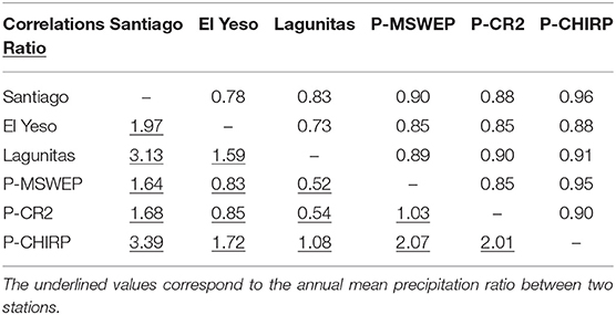
Table 2. Correlations between the different precipitation time series (statistically significant at the 95% level), and the ratios (underlined) of the mean annual precipitation between the different datasets for the 1981–2010 period.

Equilibrium Line Altitude

The latitudinal profiles of the ZIA (ZIA_lat) and the annual-mean precipitation (P_mlat) were used to obtain the latitudinal profiles of the ELA for central Chile (ELA_pmodel). An empirical relationship between the long-term annual-mean ZIA and the long-term annual-mean precipitation (P_mlat) was used for deriving the ELA_pmodel for each precipitation dataset described previously (Table 1). The mathematical expression is given by:

$\begin{array}{ll}EL{A}_{pmodel}=c_1-c_2\times Lo{g}_{10}(P_{mlat})+ZI{A}_{lat}& (3)\end{array}$

where P_mlat is the mean annual precipitation in the mountains at different latitudes, and c₁ and c₂ are the constant coefficients determined from the ELA-ZIA and the logarithm of the precipitation linear regression. The empirical model is similar to the Carrasco et al. (2005, 2008), the Condom (2002), and Condom et al. (2007) models.

To analyse annual variability of the ELA in central Chile, the time series of the annual-mean ZIA_QSD and the annual-mean accumulation of the precipitation constructed between 33 and 34°S, were used [hereafter the ELA timeseries are identified as ELA_{amodel(33−34S)}]. To assess the long-term variability of the time series, the interannual variability was filter out using the exponential smoothing Equation 4 (Rosenblüth et al., 1997):

$\begin{array}{l}{y}_t=c{x}_t+(1-c)y_{(t-1)}t=2,3,4,\dots .,n\\ z_t=c{y}_t+(1-c)z_{(t+1)}t=(n-1),n-2),\dots .,1& (4)\end{array}$

where yt is the average of the first 5–7 years of the series, zt corresponds to the final value of the first smoothing, c is the degree of smoothing (0-1), which was set to 0.20 to filter out the interannual variability while preserving the decadal behavior.

As aforementioned, field observational ELA data are scarce in Chile because they are costly in term of logistic and difficult to maintain over time. Thus, ELA has been estimated from different sources: snowline field observations; satellite and aerial photographs; accumulation area ratio (AAR) calculations; and in-situ measurements of surface mass balance using stakes deployed on the glacier surface. A list of collected ELA estimations available for the central Chilean Andes from different published sources is presented in Table 3. They were gathered to generate an estimated-observed ELA dataset profile, which was used to compare with the ELA_pmodel profiles obtained in this study. Estimated data are available from 1969 to 2015 covering the region from 27 to 39.93°S. Notwithstanding that the estimations correspond to different methods and periods; all the ELA values were plotted in a scatter chart and a polynomial curve was fitted to the data to obtain a “multidecadal estimation” of the latitudinal profile of the ELA (ELA_pref). The polynomial expression that better fits the estimated ELA_pref is:

$\begin{array}{ll}EL{A}_{pref}=1.7547\times L^3-178.97\times L^2+5701\times L-52072& (5)\end{array}$

with R² = 0.99; where L is the latitude in degrees south (L > 0), valid from 30° to 38°S (see also in Figure 7). Coefficients of Equation 5 are very sensitive to the estimated values of ELA used in the calculations; then, they might change if different estimations of ELA are considered in the analysis. In fact, the “referential ELA profile” obtained by using Equation 5 is different from the ELA_pref obtained by Carrasco et al. (2005) southward of 34°S, because new data were incorporated for constructing the updated profile in the present study.

TABLE 3

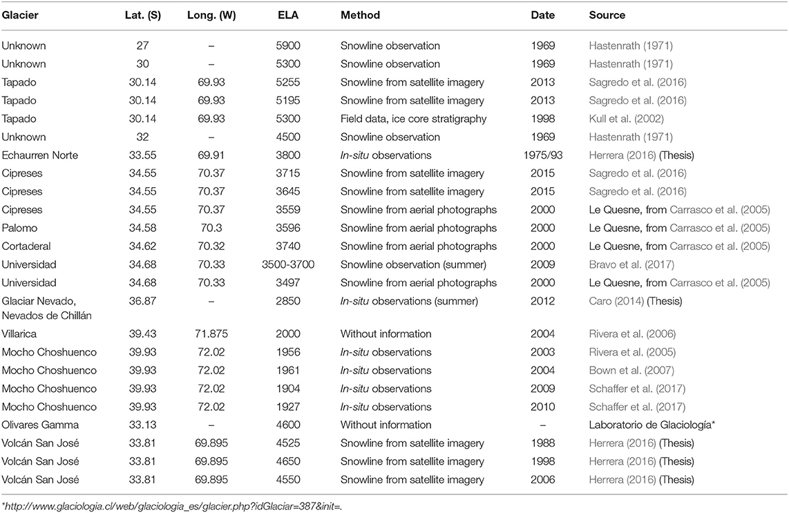
Table 3. List of the ELA estimations from in-situ measurements, from snowline field observations and snowline from satellite imagery and aerial photographs at different glaciers along the central Andes.

Then, the “referential ELA profile” (ELA_pref) is used to assess and select the ELA_pmodel, derived from the latitudinal ZIA and the different precipitation datasets (using Equation 3), that better approximates the ELA_pref. Equation 6 is used to compute the mean differences between the individual modeled ELA_pmodel and ELA_pref values.

$\begin{array}{ll}D=0.1\times \sqrt{\overline{{(x_i-y_i)}^2}}& (6)\end{array}$

Where the $\overline{{(x_i-y_i)}^2}$ is the average of the altitudinal differences between the individual ELA_pmodel (y_i) and the estimated ELA_pref (x_i).

Linear trends of the air temperature, ZIA and ELA were obtained by a simple linear regression model based on the available time series from 1958 to 2018. The uncertainties in each time series (ZIA, precipitation and ELA) were calculated using the standard error (SE) of the mean at 95% confidence interval, derived from the standard deviation (SE_mean = ± 1.95 × σ/$\sqrt{n}$). The latitudinal SE for ZIA was determined using the standard deviation of the monthly data at each areological station, and then polynomial expressions similar to Equation 1 were found for the upper and lower limit of the variability. In the same manner, latitudinal SE for precipitation was calculated using all annual accumulation datasets except the P-TMPA. The uncertainty for the ELA_amodel time series was calculated from the one obtained for ZIA and mean precipitation.

Relationship Between ELA and Surface Mass Balance at Echaurren Glacier

Additionally, the relationship between ELA_{amodel(33−34S)} and the annual surface mass balance (SMB_Annual) at Echaurren Glacier (33.55°S; 70.13°W, altitude range 3650–3880 m) (WGMS, 2017) located in the western slope of the Andes, was assessed. To do that, the ELA_{amodel(33−34S)} was expressed as the standardized anomalies of the average ELA for the 1975–2016 period, while the SMB_Annual of the glacier is expressed in m w.e.a⁻¹. The apparent relationship between the SMB_Annual and ELA_{amodel(33−34S)} suggests that a linear regression can be adjusted to both variables, which was given by Equation 7.

$\begin{array}{ll}SM{B}_{Annual}=m\times EL{A}_{amodel(33-34S)}+n& (7)\end{array}$

Also, a linear regression between the SMB_Annual and annual precipitation registered at Lagunitas station was found, resulting in Equation 8.

$\begin{array}{ll}SM{B}_{\text{A}\text{n}\text{n}\text{u}\text{a}\text{l}}=0.00032\times P+3.319& (8)\end{array}$

Assuming that the data are normally distributed, the best coefficient of correlation deployed by Equation 7 was r = −0.86 (for the 1987–2016 period), and the calibrated parameters of the linear regression between SMB_Annual and ELA_{amodel (33−34S)} were m = –0.0039 and n = 15.151. Similarly, the correlation between the precipitation and SMB_Annual for the 1975–2016 period was 0.86 (p < 0.05). These expressions were then used to reconstruct SMB_Annual back to 1958 year, when both Quintero and Lagunitas stations started to register data.

Results

Air Temperature and ZIA Variability

The standardized anomalies of the air temperatures at 850, 700, and 500 hPa along with the mean temperature anomalies for these three atmospheric levels, are presented in Figure 3A. Also, the mean of the CUSUM and Bootstrapping results for air temperature long-term analyses (red curve), the linear trends for different periods and the long-term variability (black line) obtained after applying the exponential filter (Equation 4) are included in Figure 3A. The 1976/77 climate shift is clearly detected in the air temperature time series as a significant change point (red arrow). An average air temperature increase of 1.47 ± 1.12°C (standard error at 95% confidence level) was obtained for the mid-tropospheric 850–500 hPa layer at the SDQ station during the 1958–2018 period. The temperature increases observed during that period at the 850, 700, and 500 hPa were 0.92 ± 0.08°C, 0.71 ± 0.07°C, and 0.85 ± 0.07°C, respectively, all of them statistically significant at 5% level (p < 0.05). Moreover, important multidecadal variability is observed, with a cooling of −0.91 ± 0.05°C revealed by the data between 1958 and 1976 (Figure 3A), and an overall total warming of 0.07 ± 0.02°C and 0.37 ± 0.09°C (none of them statistically significant) for the 1978–2018 and 2000–2018 periods, respectively.

The analysis of the interannual variability of ZIA (see Figure 3B) showed an increase of 127 ± 10 m (p < 0.05) for the 1958–2018 period. However, a decrease of −104 ± 14 m (p < 0.1) occurred from 1958 to 1976 (Figure 3B) and an increase of only 3 ± 28 m (non-statistically significant) between 1978 and 2018 (Figure 3B). Therefore, most of the warming observed during 1958–2018 period can be attributed to the PDO shift in 1976/77 (Giese et al., 2002). Additional changes indicate an increase of 82 ± 18 and 82 ± 15 m for the 2000–2018 and 2010–2018 periods, respectively (Figure 3B). However, these increases are not statistically significant.

Mountain Precipitation Variability

The interannual variability of the high elevation precipitation recorded in central Chile, within the 33–34°S latitudinal range, has concurrent variations with the ENSO (El Niño Southern Oscillation) cycles. On the other hand, the low frequency variability of the precipitation (multidecadal variability), obtained through Equation 4, can be associated to the PDO. The ENSO-like structure of the PDO indicates that during its cold (warm) phase the average precipitation tends to be below (above) the normal (Garreaud et al., 2019). According with the PDO Index (smooth PDO of Figure 6), a cold phase prevailed from 1944 to 1976, after that a shift to a positive phase was observed which lasted until 2007, when a cold phase started again. These PDO changes can explain the positive trend in precipitation that prevailed during the second half of the last century between 30° and 33.5°S (Carrasco et al., 2005), and the positive trend of 4%/decade (although non-significant) in snow equivalent averages of snowpack in the latitudinal range 30°-37°S, for the period 1951–2005 found by Masiokas et al. (2006). Now, a warm phase of PDO has prevailed since 2014 until present.

FIGURE 6

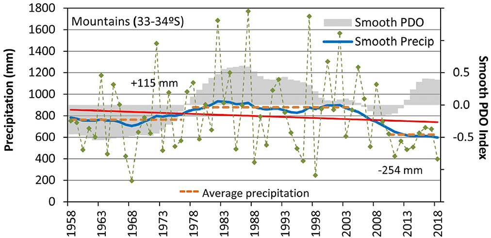
Figure 6. Interannual and decadal variability of the annual precipitation in the mountain area, between 33 and 34°S and the PDO Index.

The low frequency analysis of precipitation (blue curve of Figure 6) revealed three multidecadal cycles: a below average precipitation between 1958 until 1977, when PDO is in the negative phase, passing to above average precipitation between 1977 and 2007 when PDO is in the positive phase, to finally indicate below average precipitation from 2007 until now. In particular, the consecutive dry years registered in central Chile from 2010 to 2018 (megadrought), are equivalent to a deficit of 941.0 mm at Santiago and of 3291.5 mm at Concepción, which are almost three consecutive years of normal precipitation (as given by the 1961–1990 normal period) at both locations. The long-term variability analysis revealed an overall negative trend (non-statistically significant) with a total decrease of 19 mm over the 1958–2018 period, severely enhanced during the 2010–2018 megadrought period, when a total decline of 254 mm (29%) (Figure 6) was observed.

Observed and Modeled Latitudinal ELA Profiles

The latitudinal profile of the ZIA measurements, the ELA_pmodel, and the mean precipitation, with their respective standard errors are presented in Figure 7, along with the elevation of the central Andes crestline, and the front altitudes of some glaciers located in the western slope of the Andes. Despite the large interannual variability of ELA, according to Figure 7, the mean-ELA_pmodel fits the referential ELA_pref profile (red line in Figure 7), which is within the standard error of the mean-ELA_pmodel profile. Also, according to Figure 7, the ZIA_lat profile is lower than ELA_pref (mean-ELA_pmodel) in the zone Northern of ~35°S (~34.3°S) and higher southward from these latitudes. Therefore, the impact of the air temperature and precipitation latitudinal gradients are dominant forcing on ELA_pmodel in the region south of 35°S.

FIGURE 7

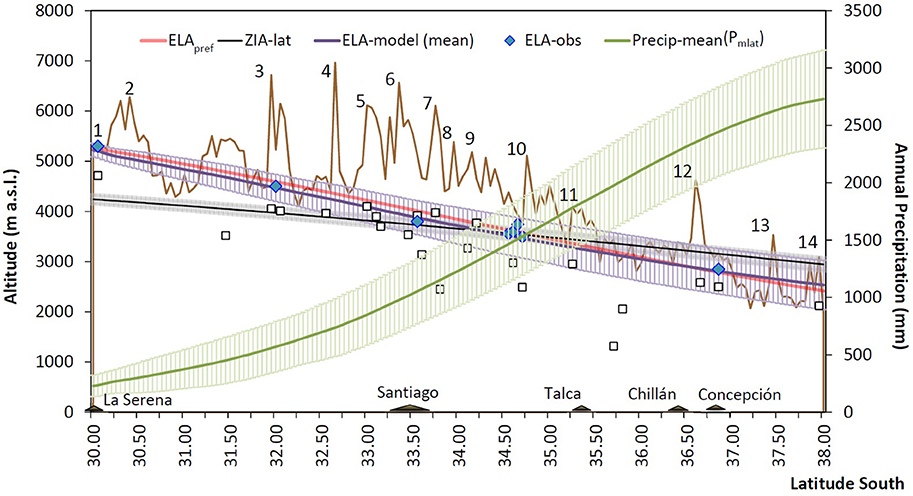
Figure 7. Latitudinal profile of the ZIA (black line), the estimated ELA (ELA_pref, red line) and ELA_model (purple curve) as determined using the ZIA and the mean precipitation data. Blue diamonds are estimated ELA reported in different articles (Table 3) and black open squares are the altitudes of some front glaciers in western Andes. The brown curve depicts the crestline of the Andes identifying some important summits (1, Co. Tapado; 2, Co. de la Majadita; 3, Mercenario; 4. Aconcagua; 5, Nevado Juncal; 6, Tupungato; 7, Co. Marmolejo; 8, Co. Colina; 9, Maipo; 10, Co. Sosneado; 11, Vc. Peteroa; 12, Vc. Domuyo; 13, Sierra Velluda; 14, Copahue).

The comparison between the ELA_pref (y axis) and the modeled ELA_pmodel derived from each precipitation dataset considered in the study, is presented in Figure 8. According to the results, the ELA_pmodel obtained from the P-CHIRPS precipitation data has the best performance in reproducing the ELA_pref, followed by ELA_pmodel based on P-MSWEP data and the ELA_pmodel obtained from the annual-mean precipitation profile. Furthermore, the ELA_pmodel derived from the P-TMPA data tends to overestimate the ELA_pref. Finally, the ELA_pmodel derived from the P-CR2, the Viale and Garreaud (2015) and the Carrasco et al. (2005) studies are the least fitted to the ELA_pref. Despite the ELA_pmodel datasets were obtained from several precipitation products, which cover periods that do not necessarily are coincident with the ELA_pref, Figure 8 shows that all ELA_pmodels fit the ELA_pref. Based on the results presented in Figure 8, the ELA_pmodel profiles derived from PCHIRPS data at different periods of time were obtained and presented in Figure 9. The results presented in Figure 9 revealed an increase in the ELA_pmodel elevation during 2010–2016 along the central Andes (30–38°S) compared to the other periods. On average, an increment of about ~133 m (ranging from ~98 to 147 m) respect to the average of the 1981–2016 period was observed, and of ~192 m (ranging from 140 to 220 m) respect to the previous 2000–2009 period. More specifically, a decadal increment of about ~369 ± 54 m occurred within the latitudinal band 33°-34°S, from the 2000–2009 to the 2010–2018 periods (see also Figure 10A). That result concurs with the megadrought that has been affecting the central and southern Chile since 2010 (Garreaud et al., 2017) and, with the high negative SMB annual rate of −1.20 ± 0.09 m w.e. a⁻¹ since 2010 found by Farias-Barahona et al. (2019).

FIGURE 8

Figure 8. Linear regressions of the different ELA_pmodel as calculated using the latitudinal precipitation datasets and the latitudinal ZIA. The estimated ELA correspond to ELA_pref obtained from Table 3. Black line is the 1:1 diagonal.

FIGURE 9

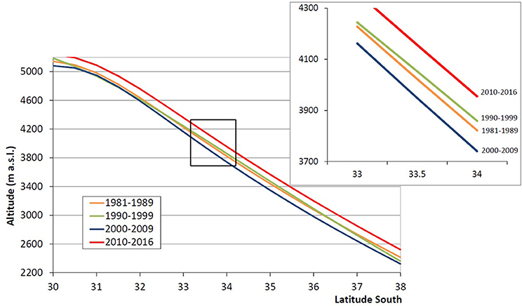
Figure 9. Latitudinal ELA_pmodel profile using CHIRPS precipitation data for different periods. The black box presents a zoom of the figure for the zone between the 33°S and 34°S.

FIGURE 10

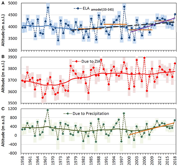
Figure 10. (A) Time series of the ELA_{amodel(33−34S)} obtained by using using Equation 3. (B) ELA_{amodel(33−34S)}, obtained from the ZIA_QSD. (C) ELA_{amodel(33−34S)} obtained from mountain precipitation between 33° and 34°S. In all graphs, diamond dashed curves are the annual variability and solid curves are long-term behaviors given by the exponential filter using Equation 4. In (A), black dashed and purple lines are the linear trends for the 1978–2018 and 2000 and 2018 periods, respectively. Brown horizontal lines are the decadal average of the ELA_{amodel(33−34S)}. In (C), The brown line is the linear trend of the ELA during the 2000–2018 period.

Annual and Long-Term Variability of ELA

The ELA_{amodel(33−34S)} for the 1958 to 2018 period was obtained using the Equation 3 (Figure 10A), forced by the mean-annual ZIA_QSD (Figure 10B) and the mean annual accumulated precipitation recorded in mountains areas near Santiago (33–34°S) (Figure 10C). The coefficients of the equation determined from the data are c₁ = 4563.9 and c₂ = 1493.2. The calibrated equation was used to obtain the time series of the mean annual ELA [ELA_{amodel(33−34S)}], and the contribution of each factor (precipitation and ZIA) in the ELA. A principal component analysis (PCA) between the ZIA_QSD, precipitation and ELA_{amodel(33−34S)} data was performed. The PCA results indicate that the linear correlation between ELA_{amodel(33−34S)} and ZIA_QSD is 0.58 (p < 0.05) and that ZIA_QSD explains about ~57% of the ELA variability, while the linear correlation between ELA_{amodel(33−34S)} and precipitation is −0.86 (p < 0.05), with precipitation explaining about ~43% of the ELA variability. These results are consistent with Saavedra et al. (2018) analyses, that studied the influence of precipitation and temperature in snow persistence in the Andes for the 2000–2016 period. To do that, they conducted a coefficient of determination analysis using precipitation and air temperature as predictors. They found that from around 33° to 34.5°S, the relative importance of precipitation and temperature were 40 and 60%, respectively (see their Figure 11).

FIGURE 11

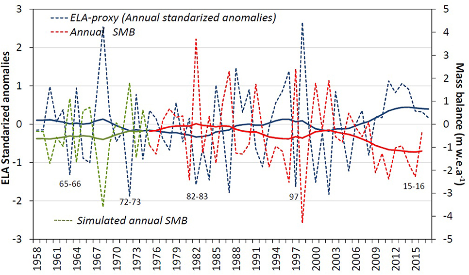
Figure 11. Annually standardized anomaly of the ELA_{amodel(33−34S)} and the SMB_Annual measured at Echaurren Glacier (dashed blue and red curve, respectively) and the long-term behavior curves obtained using Equation 4. Strong El Niño events are indicated by the years, according to the Oceanic Niño Index (ONI, https://ggweather.com/enso/oni.htm). Green dashed and solid curves from 1958 to 1975, are, respectively, the annual and smoothed SMB as reproduced by the ELA_{amodel(33−34S)} using Equation 7 with m = −0.0039 and n = 15.151.

According to the linear trend analysis of the ELA_{amodel(33−34S)}, an overall increment of ~114 ± 21 m (p < 0.1) was observed during the 1958–2018 period. A significant decrease of ~ −68 ± 12 m (non-statistically significant) was detected between 1958 and 1976, and significant increases of ~265 ± 32 m (p < 0.05) between 1978 and 2018 (Figure 10A) and of ~405 ± 55 m (p < 0.05) between 2000 and 2018 (Figure 10A) were observed after applying the exponential filter (Equation 4). That increase agrees with the generalized glacier mass balance of −0.31 ± 0.19 m w.e./year, recently reported by Dussaillant et al. (2019) between 2000 and the end of 2017 in the central Andes of Chile-Argentina (between ~31°S-~37.5°S).

ELA and the Annual Surface Mass Balance

The annual and the long-term variability of the ELA_{amodel(33−34S)} and the annual surface mass balance (SMB_Annual) at Echaurren Glacier are displayed in Figure 11. The correlation coefficient between both variables is r = −0.75 (p < 0.05), for the 1975–2016 period. According to Figure 11, the time series have considerable interannual and long-term variability, which was assessed against ENSO data. During the 1975–2016 period, the ONI index indicates the occurrence of five strong and three moderate El Niño events and five strong and two moderate La Niña events. Six (five) out of eight El Niño events concur with positive SMB_Annual (negative anomaly of the ELA), while five (three) out of seven La Niña episodes concur with negative SMB_Annual [positive anomaly of the ELA_{amodel(33−34S)}]. This is an indication of the strong relationship between glacier SMB_Annual variability (like in Echaurren) and ENSO. In the long-term, as the ELA_{amodel(33−34S)} increases in altitude, the SMB_Annual decreases, indicating an overall ice mass reduction of the Echaurren Glacier, which is likely to occur in the majority of the glaciers in the central Chilean Andes with similar geographical conditions.

To assess the performance of both: the ELA-based SMB_Annual and the precipitation-based SMB_Annual anomalies, they were compared against the observed SMB_Annual at Echaurren Glacier from 1975 to 2016 (Figure 12A). The comparison indicates that the models are skilful at representing the observed data. Therefore, the model can be used to extend the SMB_Annual analysis back to 1958 (see also Figure 11). Those results are similar to the study carried out by Masiokas et al. (2016), who modeled the observed SMB at Echaurren Glacier (reproduced in Figure 12B) using (1) a mathematical expression that relates monthly air temperature and precipitation data from El Yeso station (located 10 km south and ~1,200 m below the front glacier); and (2) the times series reconstructed from regionally averaged streamflow data, to extend the SMB back to 1909 (here reproduced from 1958).

FIGURE 12

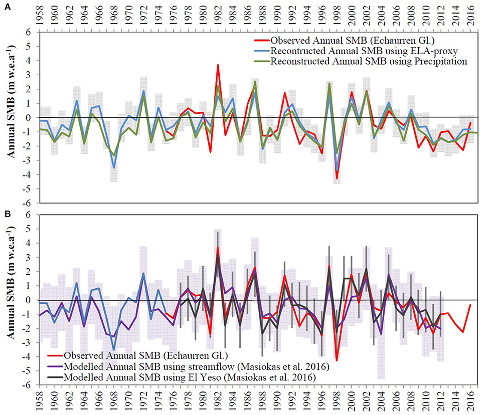
Figure 12. (A) Observed SMB_Annual at Echaurren Glacier and the reconstructed SMB_Annual using the linear relationship with ELA_amodel and mean annual precipitation on the western slope of the Andes between 33° and 34°S. The gray bars are the standard error of the time series. (B) SMB_Annual modeled using El Yeso climate data (black line) and derived from regionally average streamflow data (violet line) reproduced from Masiokas et al. (2016). Light purple bars and gray vertical lines are the modeled ± 2ε_reco (cumulative uncertainty) and 2rmse (mean standard error) (see Masiokas et al., 2016 for details).

According to the comparisons presented in Figure 12A, the reconstructed SMB using the ELA and the mean-annual precipitation data skilfully reproduce the observed annual variability of the SMB at Echaurren Glacier. Furthermore, according to Figure 12B, the reconstructed methods used by Masiokas et al. (2016) have also a good performance to simulate the observed SMB at Echaurren Glacier. For instance, the three majors observed annual SMB, which concur with the three major El Niño events (1982, 1987, and 1997), are clearly reproduced by the proxy data. Likewise, the minimum annual SMBs that concurred with La Niña events (1984, 1988, and 1998) are explained by all the models.

Discussion

The empirical relationship between ELA, ZIA, and mountain annual precipitation was used to obtain a latitudinal ELA profile for the west side of the Andes between 30 and 38°S. That model was also used to analyse the interannual and decadal variability of ELA for the 1958 and 2018 period within the 33 and 34°S region using the radiosonde data from Quintero/Santo Domingo station and the annual precipitation in mountain areas.

The latitudinal ELA_pmodel profiles constructed using the P-CHIRPS dataset during 1981–2016 period (Figure 9) reveal an overall increase of the ELA elevation in time. By calculating the averaged ELA between the 30 and 38°S, a significant difference of ~192 m (ranging from 140 to 220 m) from the 2000–2009 to the 2010–2016 period was found. More specifically, an increase in ~207 m occurred within the latitudinal band 33°-34°S, between the same two periods. The aforementioned increases in ELA_pmodel concurs with the persistent megadrought that has been affecting the central and southern regions of Chile since 2010 (Garreaud et al., 2017).

Results of Carrasco et al. (2008) previous work indicated that Central Chilean ELA (given by QSD station) rose ~54 and 191 m during the 1958–2006 and 1978–2006 periods, respectively. Now, the linear trend of ELA_{amodel(33−34S)} during the 1958–2018 period indicates a total increment of ~114 ± 21 m (p < 0.1). Most of that increment can be attributed to the climate shift leaded by the PDO cyclicity. Moreover, a decrease of −68 ± 12 m in the ELA_{amodel(33−34S)} occurred between 1958 and 1976, concurrent with a negative phase of PDO. On the other hand, an overall increase of ~265 ± 32 m (p < 0.05) took place between 1978 and 2018 and of ~405 ± 55 m (p < 0.05) between 2000 and 2018. That trend is related to the significant increase of 369 m in ELA between the 2000–2009 and the 2010–2018 periods. The increases in ELA during the last decade are mostly explained by the precipitation factor (the decrease during the megadrought; Garreaud et al., 2019) (Figure 10C), rather than the ZIA which even shows a slight decline after 2000 (Figure 10B). Finally, according to the long-term analyses, the variability of ELA is associated with changes in the ZIA and precipitation.

A correlation factor of r = −0.86 (for the 1987–2016 period) was found between ELA_{amodel(33−34S)} and the annual surface mass balance (SMB_Annual) at Echaurren Glacier. The mathematical expression of this correlation was applied to reconstruct the SMB_Annual using the ELA_{amodel(33−34S)} annual time series back to 1958. A comparison among the reconstructed SMB_Annual obtained by Masiokas et al. (2016), the ELA_{amodel30−34°S} and precipitation model derived in the present study and the observed SMB at Echaurren glacier, indicates that all of them are skilful at reproducing the observations. Besides, moderate and strong El Niño events occurred during the 1963–64 and 1972–73 years, which could explain the observed positive SMB in the 1963 and 1972 years. Also, the extreme drought that affected central Chile in 1968 (González-Reyes, 2016) could explain the observed negative SMB (Figure 12). All the aforementioned events are better reproduced by the ELA_amodel obtained in this study than the other reconstructions. Nonetheless, the four reconstruction methods have a good performance for simulating the variability of the observed SMB at Echaurren Glacier, and they contribute to improve the understanding of the interannual variability of SMB back to 1958.

Conclusion

Glaciers and winter snow in the Andes are fundamental sources of freshwater for human activities such as agriculture, hydropower generation, mining, drinkable water, and for the conservation of the ecosystems. Because of the sensitivity of glaciers to changes in temperature and precipitation, they are good indicators for climate change detection. However, direct observations of glacier surface mass balance (SMB) and snow cover in the Andes are scarce and often of short length. Different methods and techniques based on models and satellite data have been used to overcome this shortcoming. For instance, SMB can be estimated using the annual equilibrium line altitude (ELA). However, direct measurements of the ELA require field campaigns to remote locations, which are costly in term of logistic and difficult to maintain overtime. Considering that, the present study shows that indirect measurements of ELA (like the ELA_model) arise as a prominent alternative to be used as a proxy for monitoring the behavior of glaciers in those areas where permanent observations of vertical air temperature profiles and mountain precipitation data are available.

Therefore, the empirical relationship between air temperature and precipitation data can provide permanent annual estimations of the ELA, which can be calibrated with occasional field campaigns. Additionally, the good correlation between annual ELA_amodel and annual observations of SMB at Echaurren Glacier suggests that annual ZIA and mountain precipitation can be used as a proxy for monitoring the ELA in central Chilean Andes, method that can be extended to other places where these data is available too.

Although the ELA_model and the SMB of Echaurren Glacier present good correlations during the period considered in this assessment, that result could change if another time window is assessed. Since glaciers can adjust their size to achieve an equilibrium with climate, the same ELA_model value (or variation concerning the mean) could be associated with an entirely different SMB, depending on the degree of adjustment of the glacier to the climate conditions. Therefore, it is important to mention that despite this model is skilful at representing ELA, only a fraction of its total variance is explained, and future work should explore the influence of other factors like wind, radiation and morpho-topographic variables such as bedrock geology, slope and basin orientation, among others.

Because the ELA-model adjusted in this assessment is based on the annual precipitation accumulated in mountain areas and the altitude of the zero isotherm, and that both variables can be obtained from numerical climate simulation models for present and future scenarios, past and future glacier changes can be indirectly study using it.

Author Contributions

GC and JC designed the study. IB, JC, and PB processed and analyzed the data. JC and IB along with the other authors worked in the manuscript.

Funding

This study has been partially financed by Conicyt through the Fondecyt Project N° 1151034 and the Conicyt-Anillo ACT-1410. The comments and suggestions from the handling editor and reviewers significantly improved the manuscript and are greatly appreciated.

Conflict of Interest

The authors declare that the research was conducted in the absence of any commercial or financial relationships that could be construed as a potential conflict of interest.

References

Adam, J. C., Clark, E. A., Lettenamier, D. P., and Wood, E. F. (2006). Correction of global precipitation products for orographic effects. J. Climate 19, 15–38. doi: 10.1175/JCLI3604.1

CrossRef Full Text | Google Scholar

Adler, R. F., Huffman, G. J., Chang, A., Ferraro, R., Xie, P.-P., Janowiak, J., et al. (2003). The version-2 global precipitation climatology project (GPCP) monthly precipitation analysis (1979–Present). J. Hydrometeorol. 4, 1147–1167. doi: 10.1175/1525-7541(2003)004<1147:TVGPCP>2.0.CO;2

CrossRef Full Text | Google Scholar

Alvarez-Garreton, C., Mendoza, P. A., Boiser, J. P., Addor, N., Galleguillos, M., Zambrano-Bigiarini, M., et al. (2018). The CAMELS-CL dataset:catchment atributes and meteorology for large samples studies _ Chile DATASET. Hydrol. Earth Sys. Sci. 22, 5817–5846. doi: 10.5194/hess-22-5817-2018

CrossRef Full Text | Google Scholar

Ayala, A., Pellicciotti, F., MacDonell, S., McPhee, J., Vivero, S., Campos, C., et al. (2016). Modelling the hydrological response of debris-free and debris-covered glaciers to present climatic conditions in the semiarid Andes of central Chile. Hydrol. Process. 30, 4036–4058. doi: 10.1002/hyp.10971

CrossRef Full Text | Google Scholar

Balsamo, G., Albergel, C., Beljaars, A., Boussetta, S., Brun, E., Cloke, H., et al. (2015). ERAInterim/Land: a global land surface reanalysis data set. Hydrol. Earth Syst. Sci. 19, 389–407. doi: 10.5194/hess-19-389-2015

CrossRef Full Text | Google Scholar

Barcaza, G., Nussbaumer, S. U., Tapia, G., Valdes, J., Garcia, J. L., Videla, Y., et al. (2017). Glacier inventory and recent glacier variations in the Andes of Chile, South America. Ann. Glaciol. 58, 166–180. doi: 10.1017/aog.2017.28

CrossRef Full Text | Google Scholar

Beck, H. E., van Dijk, A. I. J. M., Levizzani, V., Schellekens, J., Miralles, D. G., Martens, B., et al. (2017). MSWEP: 3-hourly 0.25° global gridded precipitation (1979–2015) by merging gauge, satellite, and reanalysis data. Hydrol. Earth Syst. Sci. 21, 589–615. doi: 10.5194/hess-21-589-2017

CrossRef Full Text | Google Scholar

Boisier, J. P., Alvarez-Garreton, C., Cordero, R. R., Damiani, A., Gallardo, L., Garreaud, R. D., et al. (2018). Anthropogenic drying in central-southern Chile evidenced by long-term observations and climate model simulations. Elem. Sci. Anthropocene 6:74. doi: 10.1525/elementa.328

CrossRef Full Text | Google Scholar

Boisier, J. P., Rondanelli, R., Garreaud, R., and Muñoz, F. (2016). Anthropogenic and natural contributions to the Southeast Pacific precipitation decline and recent megadrought in central Chile. Geophys. Res. Lett. 43, 413–421. doi: 10.1002/2015GL067265

CrossRef Full Text | Google Scholar

Bown, F., Rivera, A., Acuña, C., and Casassa, G. (2007). Recent glacier mass balance calculations at Volcán Mocho-Choshuenco (40°S), Chilean Lake District. IAHS Publ. 318, 143–152.

Google Scholar

Braun, M. H., Malz, P., Sommer, C., Farias-Barahona, D., Sauter, T., Casassa, G., et al. (2019). Contrasting glacier elevation and mass changes in South America. Nat. Climate Change. 9, 130–136. doi: 10.1038/s41558-018-0375-7

CrossRef Full Text | Google Scholar

Bravo, C., Loriaux, T., Rivera, A., and Brock, B. W. (2017). Assessing glacier melt contribution to streamflow at Universidad Glacier, central Andes of Chile. Hydrol. Earth Syst. Sci. 21, 3249–3266. doi: 10.5194/hess-21-3249-2017

CrossRef Full Text | Google Scholar

Burger, F., Brock, B., and Montecinos, A. (2018). Seasonal and elevational contrasts in temperature trends in Central Chile between 1979 and 2015. Glob. Planet. Change, 162, 136–147. doi: 10.1016/j.gloplacha.2018.01.005

CrossRef Full Text | Google Scholar

Caro, D. (2014). Estudios glaciológicos en Los Nevados de Chillán (Undergraduate Thesis). Santiago: Universidad de Chile, 131 pp.

Google Scholar

Carrasco, J. F., Casassa, G., and Quintana, J. J. (2005). Changes of the 0 C isotherm and the equilibrium line altitude in central Chile during the last quarter of the 20th century. Hydrol. Sci. J. 50, 933–948. doi: 10.1623/hysj.2005.50.6.933

CrossRef Full Text | Google Scholar

Carrasco, J. F., Osorio, R., and Casassa, G. (2008). Secular trend of the equilibrium-line altitude on the western side of the southern Andes, derived from radiosonde and surface observations. J. Glaciol. 54, 538–550. doi: 10.3189/002214308785837002

CrossRef Full Text | Google Scholar

Casassa, G., López, P., Pouyaud, B., and Escobar., F. (2009). Detection of changes in glacial run-off in alpine basins: examples from North America, the Alps, central Asia and the Andes. Hydrol. Process. 23, 31–41. doi: 10.1002/hyp.7194

CrossRef Full Text | Google Scholar

Casassa, G., Rivera, A., Haeberli, W., Jones, G., Kaser, G., Ribstein, P., et al. (2007). Current status of Andean glaciers. Glob. Planet. Change, 59, 1–9. doi: 10.1016/j.gloplacha.2006.11.013

CrossRef Full Text | Google Scholar

Chinn, T. J. (1999). New Zealand glacier response to climate change of the past 2 decades. Glob. Planet. Change, 22, 155–168. doi: 10.1016/S0921-8181(99)00033-8

CrossRef Full Text | Google Scholar

Christidis, N., Stott, P. A., Zwiers, F. W., Shiogama, H., and Nozawa, T. (2010). Probabilistic estimates of recent changes in temperature: a multi-scale attribution analysis. Climate Dyn. 34, 1139–56. doi: 10.1007/s00382-009-0615-7

CrossRef Full Text | Google Scholar

Cogley, J. G., Hock, R., Rasmussen, L. A., Arent, A. A., Bauder, A., Braithwaite, R. J., et al. (2011). “Glossary of glacier mass balance and related terms,” in IHP-VII Technical Documents in Hydrology No. 86, IACS Contrib. No. 2, UNESCO-IHP (Paris).

Google Scholar

Condom, T. (2002). Dynamiques d'extension lacustre et glaciaire associées aux modifications du climat dans les Andes Centrales (Ph. D. Thesis). Paris: University of Paris VI-Pierre et Marie Curie.

Google Scholar

Condom, T., Coudrain, A., Sicart, J. E., and Thery, S. (2007). Computation of the space and time evolution of equilibrium-line altitudes on Andean glaciers (10 degrees N-55 degrees S). Glob. Planet. Change, 59, 189–202. doi: 10.1016/j.gloplacha.2006.11.021

CrossRef Full Text | Google Scholar

Cortés, G., and Margulis, S. (2017). Impacts of El Niño and La Niña on interannual snow accumulation in the Andes: results from a high-resolution 31-year reanalysis. Geophys. Res. Lett. 44, 6859–6867. doi: 10.1002/2017GL073826

CrossRef Full Text | Google Scholar

Dussaillant, I., Berthier, E., Brun, F., Masiokas, M., Hugonnet, R., Favier, V., et al. (2019). Two decades of glacier mass loss along the Andes. Nat. Geosci. 12, 802–808. doi: 10.1038/s41561-019-0432-5

CrossRef Full Text | Google Scholar

Falvey, M., and Garreaud, R. (2007). Wintertime precipitation episodes in central Chile: associated meteorological conditions and orographic influences. J. Hydrometeorol. 8, 171–193. doi: 10.1175/JHM562.1

CrossRef Full Text | Google Scholar

Falvey, M., and Garreaud, R. (2009). Regional cooling in a warming world: recent temperature trends in the southeast Pacific and along the west coast of subtropical South America (1979-2006). J. Geophys. Res. Atmos. 114, 1–16. doi: 10.1029/2008JD010519

CrossRef Full Text | Google Scholar

Farias-Barahona, D., Vivero, S., Casassa, G., Schaefer, M., Burger, F., Seehaus, T., et al. (2019). Geodetic mass balances and área changes of Echaurren Norte Glacier (Central Andes, Chile) between 1955 and 2015. Remote Sens. 11:260. doi: 10.3390/rs11030260

CrossRef Full Text | Google Scholar

Favier, V., Falvey, M., Rabatel, A., Pradeiro, E., and López, D. (2009). Interpreting discrepancias between discharge and precipitation in high-altitude area of Chile's Norte Chico region (26-32°S). Water Resour. Res. 45:W02424. doi: 10.1029/2008WR006802

CrossRef Full Text | Google Scholar

Foster, J., Hall, D. K., Kelly, R., and Chiu, L. (2009). Seasonal snow extent and snow mass in South America using SMMR and SSM/I passive microwave data (1979-2006). Remote Sens. Environ. 113, 291–305. doi: 10.1016/j.rse.2008.09.010

CrossRef Full Text | Google Scholar

Funk, C., Peterson, P., Landsfeld, M., Pedreros, D., Verdin, J., Shukla, S., et al. (2015). The climate hazards infrared precipitation with stations – A new environmental record for monitoring extremes. Sci. Data 2:150066. doi: 10.1038/sdata.2015.66

PubMed Abstract | CrossRef Full Text | Google Scholar

Garreaud, R. D. (2009). The Andes climate and weather. Adv. Geosci. 22, 3–11. doi: 10.5194/adgeo-22-3-2009

CrossRef Full Text | Google Scholar

Garreaud, R. D., Alvarez-Garreton, C., Barichivich, J., Boisier, J. P., Christie, D., Galleguillos, M., et al. (2017). The 2010-2015 mega drought in Central Chile: impacts on regional hydroclimate and vegetation. Hydrol. Earth Syst. Sci. Discuss. 2017, 1–37. doi: 10.5194/hess-2017-191

CrossRef Full Text | Google Scholar

Garreaud, R. D., Boiser, J. P., Rondanelli, R., Montecinos, A., Sepúlveda, H. H., and Veloso-Aguila, D. (2019). The Central Chile Mega Drough (2010-2018): a climate dynamics perspective. Int. J. Climatol. 39, 1–19. doi: 10.1002/joc.6219

CrossRef Full Text | Google Scholar

Giese, B. S., Urizar, S. C., and Fuckar, N. S. (2002). Southern Hemisphere origins of the 1976 climate shift. Geophys. Res. Lett. 29:1014. doi: 10.1029/2001GL013268

CrossRef Full Text | Google Scholar

González-Reyes, A. (2016). Ocurrencia de eventos de sequía en la ciudad de Santiago de Chile desde mediados del Siglo XIX. Rev. Geog. Norte Grande 64, 21–32. doi: 10.4067/S0718-34022016000200003

CrossRef Full Text | Google Scholar

Hartmann, D. L., Klein Tank, A. M. G., Rusticucci, M., Alexander, L. V., Bronimann, S., Charabi, Y. A-.R., et al. (2013). “Observations: atmosphere and surface,” in Climate Change 2013: The Physical Science Basis. Contribution of Working Group I to the Fifth Assessment Report of the Intergovernmental Panel on Climate Change, eds T. F. Stocker, D. Qin, G.-K. Plattner, M. Tignor, S. K. Allen, J. Buschung, et al. (Cambridge, UK; New York, NY: Cambridge University Press), 159–254.

Google Scholar

Hastenrath, S. (1971). On the Plestocene snow-line depression in the arid regions of the South American Andes. J. Glaciol. 3, 255–267. doi: 10.1017/S0022143000013228

CrossRef Full Text | Google Scholar

Herrera, M. (2016). Estimación de las altitudes de las líneas de equilibrio en glaciares de montaña para el último cilo glacial-interglacial en los Andes de Santiago, Chile central (Ph.D. Thesis). Santiago: Universidad de Chile, 202 pp.

Google Scholar

Khan, A., Chatterjee, S., Bisai, D., and Barman, N. K. (2014). Analysis of change point in surface temperature time series using Cumulative Sum Chart and Bootstrapping for Asonsol weather observation station, West Bengal, India. Amer. J. Climate Change 3, 83–94. doi: 10.4236/ajcc.2014.31008

CrossRef Full Text | Google Scholar

Kull, C., Grosjean, M., and Veit, H. (2002). Modelling modern and late Pleistocene glacio-climatological conditions in the North Chilean Andes (29-30°S). Clim. Change 52, 115–160. doi: 10.1023/A:1013746917257

CrossRef Full Text | Google Scholar

Le Quesne, C., Acuña, C., Boninsegna, J., Rivera, A., and Barichivich, J. (2009). Long-term glacier variations in the Central Andes of Argentina and Chile, inferred from historical records and tree-ring reconstructed precipitation. Palaeogeogr. Palaeoclimatol. Palaeoecol. 281, 334–344. doi: 10.1016/j.palaeo.2008.01.039

CrossRef Full Text | Google Scholar

Leiva, J. C., Cabrera, G. A., and Lenzano, L. E. (2007). 20 years of mass balances on the Piloto Glacier, Las Cuevas river basin, Mendoza, Argentina. Glob. Planet. Change 59, 10–16. doi: 10.1016/j.gloplacha.2006.11.018

CrossRef Full Text | Google Scholar

Malmros, J., Mernild, S., Wilson, R., Tagesson, T., and Fensholt, R. (2018). Snow cover and albedo changes in the central Andes of Chile and Argentina from daily MODIS observations (2000-2016). Remote Sens. Environ. 209, 240–252. doi: 10.1016/j.rse.2018.02.072

CrossRef Full Text | Google Scholar

Malmros, J., Mernild, S., Wilson, R., Yde, J., and Fensholt, R. (2016). Glacier area changes in the central Chilean and Argentinean Andes 1955-2013/14. J. Glaciol. 62, 391–401. doi: 10.1017/jog.2016.43

CrossRef Full Text | Google Scholar

Masiokas, M. H., Christie, D. A., Le Quesne, C., Pitte, P., Ruiz, L, Villalba, R., et al. (2016). Reconstructing the annual mass balance of the Echaurtren Norte glacier (Central Andes, 33.5°S) using local and regional hydroclimatic data. Cryosphere 10, 927–940. doi: 10.5194/tc-10-927-2016

CrossRef Full Text | Google Scholar

Masiokas, M. H., Villalba, R., Luckman, B. H., Le Quesne, C., and Aravena, J. C. (2006). Snowpack variations in the central Andes of Argentina and Chile, 1951-2005: large-scale atmospheric influences and implications for water resources in the region. J. Clim. 19, 6334–6352. doi: 10.1175/JCLI3969.1

CrossRef Full Text | Google Scholar

Masiokas, M. H., Villalba, R., Luckman, B. H., and Mauget, S. (2010). Intra- to multidecadal variations of snowpack and streamflow records in the Andes of Chile and Argentina between 30° and 37° S. J. Hydrometeorol. 11, 822–831. doi: 10.1175/2010JHM1191.1

CrossRef Full Text | Google Scholar

Mernild, S. H., Liston, G. E., Hiemstra, C. A., Malmros, J. K., Yde, J. C., and McPhee, J. (2016). The Andes Cordillera. Part I: snow distribution, properties, and trends (1979–2014). Int. J. Climatol. 37, 1680–1698 doi: 10.1002/joc.4804

CrossRef Full Text | Google Scholar

Migliavacca, F., Confortola, G., Soncini, A., Senese, A., Diolaiuti, G. A., Smiraglia, C., et al. (2015). Hydrology and potential climate changes in the Rio Maipo (Chile). Geografia Fisica E Dinamica Quaternaria 38, 155–168. doi: 10.4461/GFDQ.2015.38.14

CrossRef Full Text | Google Scholar

Montecinos, A., and Aceituno, P. (2003). Seasonality of the ENSO-related rainfall variability in central Chile and associated circulation anomalies. J. Clim. 16, 281–296. doi: 10.1175/1520-0442(2003)016<0281:SOTERR>2.0.CO;2

CrossRef Full Text | Google Scholar

Pellicciotti, F., Ragettli, S., Carenzo, M., and McPhee, J. (2014). Changes of glaciers in the Andes of Chile and priorities for future work. Sci. Total Environ. 493, 1197–1210. doi: 10.1016/j.scitotenv.2013.10.055

PubMed Abstract | CrossRef Full Text | Google Scholar

Peña, H., and Nazarala, B. (1987). Snowmelt-Runoff Simulation Model of a Central Chile Andean Basin With Relevant Orographic Effects. Vancouver, BC: IAHS-AISH publication, 161–172.

Google Scholar

Quintana, J., and Aceituno, P. (2012). Changes in the rainfall regime along the extratropical west coast of South America (Chile): 30-43 degrees S. Atmosfera 25, 1–22.

Google Scholar

Rabatel, A., Dedieu, J.-P., and Vincent, C. (2005). Using remote-sensing data to determine equilibrium-line altitude and mass-balance time series:validation on three French glaciers, 1994-2002. J. Glaciol. 51, 539–546. doi: 10.3189/172756505781829106

CrossRef Full Text | Google Scholar

Ragettli, S., and Pellicciotti, F. (2012). Calibration of a physically based, spatially distributed hydrological model in a glacierized basin: on the use of knowledge from glaciometeorological processes to constrain model parameters. Water Resour Res. 48, 1–20. doi: 10.1029/2011WR010559

CrossRef Full Text | Google Scholar

Rivera, A., Acuña, C., and Casassa, G. (2006). “Glacier variations in central Chile (32°S-41°S),” in Glacier Science and Environmental Change, edP. G. Knight (Oxford: Blackwell), 246–247. doi: 10.1002/9780470750636.ch49

CrossRef Full Text | Google Scholar

Rivera, A., Acuna, C., Casassa, G., and Bown, F. (2002). Use of remotely sensed and field data to estimate the contribution of Chilean glaciers to eustatic sea-level rise. Ann. Glaciol. 34, 367–372. doi: 10.3189/172756402781817734

CrossRef Full Text | Google Scholar

Rivera, A., Casassa, G., Acuña, C., and Clavero, J. (2005). Glacier shrinkage and negative mass balance in the Chilean Lake District (40°S). Hydrol. Sci. J. 50, 963–974. doi: 10.1623/hysj.2005.50.6.963

CrossRef Full Text | Google Scholar

Ropelewski, C. F., Janowiak, J. E., and Halpert, M. S. (1984). The Climate Anomaly Monitoring System (CAMS). Climate Analysis Center, NSW, NOAA. Washigton, DC, 39.

Google Scholar

Rosenblüth, B., Fuenzalida, H., and Aceituno, P. (1997). Recent temperature variations in southern South America. Int. J. Climatol. 17, 67–85. doi: 10.1002/(SICI)1097-0088(199701)17:1<67::AID-JOC120>3.0.CO;2-G

CrossRef Full Text | Google Scholar

Saavedra, F. A., Kampf, S. K., Fassnacht, S. R., and Sibold, J. S. (2018). Changes in Andes snow cover from MODIS data, 2000-2016. Cryosphere 12, 1027–1047. doi: 10.5194/tc-12-1027-2018

CrossRef Full Text | Google Scholar

Sagredo, E. A., Lowel, T. V., Kelly, M. A., Rupper, S., Aravena, J. C., Ward, D. J., et al. (2016). Equilibrium line altitude along the Andes during the Last millennium: paleoclimatic implications. The Holocene. 1-15. doi: 10.1177/0959683616678458

CrossRef Full Text | Google Scholar

Schaffer, M., Rodriguez, J. L., Scheiter, M., and Casassa, G. (2017). Climate and surface mass balance of Mocho Glacier, Chilean Lake District, 40°S. J. Glaciol. 63, 218–228. doi: 10.1017/jog.2016.129

CrossRef Full Text | Google Scholar

Stehr, A., and Aguayo, M. (2017). Snow cover dynamics in Andes watersheds of Chile (32.0-39.5°S) during the years 2000-2016. Hydrol. Earth Syst. Sci. 21, 5111–5126. doi: 10.5194/hess-21-5111-2017

CrossRef Full Text | Google Scholar

Taylor, W. (2000). Change-Point Analyzer 2.3 Software Package. Taylor Enterprises Inc., Libertyville. Available online at: https://variation.com/product/change-point-analyzer/ (accessed October 9, 2019)

Google Scholar

Viale, M., and Garreaud, R. (2015). Orographic effects of the subtropical and extratropical Andes on upwind precipitating clouds. J. Geophys. Res. Atmos. 120, 4962–4974. doi: 10.1002/2014JD023014

CrossRef Full Text | Google Scholar

Viale, M., Valenzuela, R., Garreaud, R., and Ralph, F. (2018). Impacts of atmospheric rivers on precipitation in Southern South America. J. Hydrometeor. 18. 1671–1686. doi: 10.1175/JHM-D-18-0006.1

CrossRef Full Text | Google Scholar

Vuille, M. E, Franquist, R., Garreaud, W., and Lavado Casimiro Caceres, B. (2015). Impact of the global warming hiatus on Andean temperature. J. Geophys. Res. Atmos. 120, 3745–3757. doi: 10.1002/2015JD023126

CrossRef Full Text | Google Scholar

WGMS (2017). “Updated, and earlier reports: Global Glacier Change Bulletin No. 2 (2014-2015),” in ICSU(WDS)/IUGG(IACS)/UNEP/UNESCO/WMO, eds M. Zemp, S. U. Nussbaumer, I. Gärtner-Roer, J. Huber, H. Machguth, F. Paul, et al. (Zurich: World Glacier Monitoring Service), 244.

Google Scholar