Abstract
The applicability of optical satellite data to quantify coastal erosion across the Arctic is limited due to frequent cloud cover. Synthetic Aperture Radar (SAR) may provide an alternative. The interpretation of SAR data for coastal erosion monitoring in Arctic regions is, however, challenging due to issues of viewing geometry, ambiguities in scattering behavior and inconsistencies in acquisition strategies. In order to assess SAR applicability, we have investigated data acquired at three different wavelengths (X-, C-, L-band; TerraSAR-X, Sentinel-1, ALOS PALSAR 1/2). In a first step we developed a pre-processing workflow which considers viewing geometry issues (shoreline orientation, incidence angle relationships with respect to different landcover types). We distinguish between areas with foreshortening along cliffs facing the sensor, radar shadow along cliffs facing away and traditional land-water boundary discrimination. Results are compared to retrievals from Landsat trends. Four regions which feature high erosion rates have been selected. All three wavelengths have been investigated for Kay Point (Canadian Beaufort Sea Coast). C- and L-band have been studied at all sites, including also Herschel Island (Canadian Beaufort Sea Coast), Varandai (Barents Sea Coast, Russia), and Bykovsky Peninsula (Laptev Sea coast, Russia). Erosion rates have been derived for a 1-year period (2017–2018) and in case of L-band also over 11 years (2007–2018). Results indicate applicability of all wavelengths, but acquisitions need to be selected with care to deal with potential ambiguities in scattering behavior. Furthermore, incidence angle dependencies need to be considered for discrimination of the land-water boundary in case of L- and C-band. However, L-band has the lowest sensitivity to wave action and relevant future missions are expected to be of value for coastal erosion monitoring. The utilization of trends derived from Landsat is also promising for efficient long-term trend retrieval. The high spatial resolution of TerraSAR-X staring spot light mode (<1 m) also allows the use of radar shadow for cliff-top monitoring in all seasons. Derived retreat rates agree with rates available from other data sources, but the applicability for automatic retrieval is partially limited. The derived rates suggest an increase of erosion at all four sites in recent years, but uncertainties are also high.
1. Introduction
Arctic regions are some of the most rapidly changing environments on Earth, and their coastlines are especially vulnerable to climate change due to permafrost thaw and marine changes (Lantuit, 2008; Overland et al., 2019; Nielsen et al., 2020). The latter includes decrease in sea ice extent due to warming temperatures and change in wave action (driven by length of open water season and sea ice concentration anomalies, Nielsen et al., 2020). They impact thermo-denudation and thermo-abrasion along the coast. The annual erosion rates at the Alaskan and northwest Canadian Arctic coastlines are among the highest in the world, but Siberian coastlines also show high rates (Frederick et al., 2016). These irreversible coastal changes are a threat to communities and wildlife in those areas. Communities have needed to be relocated, and houses and archaeological sites have been damaged (Jones et al., 2008; Arp et al., 2010; Frederick et al., 2016; Radosavljevic et al., 2016; Irrgang et al., 2019). In addition to these directly visible effects, the erosion mobilizes significant amounts of carbon and contaminants (e.g., Steele et al., 2008; Couture et al., 2018; Schuster et al., 2018; Overland et al., 2019). There is a clear need to quantify erosion regularly on circumpolar scale, but available studies focus on local to regional level. A first account for circumpolar rates has been published in 2012 (Lantuit et al., 2012). It is based on published rates from in situ measurements and partially from satellite data from a wide range of studies, which have been aggregated for coast segments to tackle scale differences. That study provides a first account of circumpolar coastal dynamics, but is inconsistent. Moreover, global initiatives on quantification of shore line changes based solely on satellite data omit the Arctic (e.g., Mentaschi et al., 2018).
Arctic coastal erosion has been monitored through airborne and spaceborne optical imagery or in situ measurements (e.g., Obu et al., 2016; Irrgang et al., 2018; Cunliffe et al., 2019). In situ measurements only cover small areas, and optical images can be unreliable due to frequent cloud cover in the Arctic (Stettner et al., 2017; Zwieback et al., 2018). Microwave radiation on the other hand is barely affected by the atmosphere, and does not rely on solar illumination, which can be especially useful for monitoring Arctic regions (Jones and Vaughan, 2010). This has motivated recent interest in using microwave technologies like Synthetic Aperture Radar (SAR) to monitor Arctic regions. The interpretation of SAR data for coastal erosion in Arctic regions is, however, challenging (Stettner et al., 2017). Differential SAR interferometry (DInSAR) and SAR interferometry (InSAR) have been successfully used to measure gradual surface displacement in Arctic environments (e.g., Liu et al., 2012; Strozzi et al., 2018). However, detecting mass movements is difficult, because repeat-pass interferometry methods are not effective in rapidly changing terrain such as the Arctic coasts. The changes between the satellite revisit times are too large in comparison to the SAR wavelength, and no useful correlation can be found between the images (Short et al., 2011; Zwieback et al., 2018). Therefore, Stettner et al. (2017) introduced a backscatter-based threshold method with TerraSAR-X images to classify and evaluate inter- and intra-annual cliff-top erosion rates. The high backscatter difference between tundra, water and steep cliffs facing the sensor justifies the simple approach. Unfortunately, only a limited number of high spatial resolution (in respect to the erosion rates) SAR acquisitions of the Arctic region exist. A further challenge is the limitation of the approach to steep cliffs facing toward the sensor. A different method is needed for cliffs facing away and coasts without steep cliffs. As an alternative, to cover also all other parts of the coastline, the separability between the land-water boundary needs to be investigated. Banks et al. (2014) analyzed the backscatter characteristics of Arctic shore and near-shore landcover types for C-band images in various incidence angle ranges and polarizations. They found that the separability between sand and water backscatter in C-band strongly depends on the incidence angle and polarization. Differences in applicability of certain wavelengths are also to be expected due to their varying sensitivity to waves on the water and surface roughness (modified by vegetation and snow; examples from Arctic sites in Stettner et al., 2018; Bartsch et al., 2020) on land, which leads to ambiguities. Wet snow appears similar to water (low backscatter), as do radar shadow areas. Waves and sea ice show similar or even higher backscatter than typical undisturbed tundra. An additional challenge poses the variation of spatial resolution across commonly used SAR spaceborne missions.
This study tests the accuracy and transferability of the threshold-based method proposed by Stettner et al. (2017) for comparably low resolution PALSAR/PALSAR-2 L-band and Sentinel-1 C-band images in addition to high-resolution TerraSAR-X X-band acquisitions. The overall goal is to identify options for operational mapping of coastal erosion along Arctic coasts. This requires the analyses of the land-water boundary in addition to represent all coast types.
The first objective is therefore to implement and demonstrate a landcover classification scheme for X-, C- and L-band data building on the approach suggested by Stettner et al. (2017). Specifically, the classification should correctly identify steep coasts, land, and water surfaces for applicability across various coast types. To achieve this, the classification approach must account for the landcover specific angular dependence in the classification step. Where available, different polarization needs to be assessed. Previously, thresholds have been determined only visually (Stettner et al., 2017). A quantitative approach is, however, required.
The second objective is to demonstrate the use of the proposed classifications to analyze coastline change in the Arctic. Specifically, annual coastline movement rates are calculated for steep cliff coastlines. The accuracy of these estimates is assessed by comparison with trends derived from multi-spectral data, published results from previous studies, and by cross-comparisons between sensors within this study.
2. Materials and Methods
2.1. Study Areas and Reference Data for Coastal Erosion Rates
In order to judge the utility of different SAR parameters to detect and measure coastal erosion, we conducted our analysis in areas where coastal erosion has been measured before. This study focuses on four coastal sites in three regions with existing records of comparably high erosion rates from previous studies: two sites at the Canadian Beaufort Sea (Herschel Island, 139.3°W 69.6°N; Kay Point, 138.4°W 69.3°N), one at the Russian Laptev Sea (Bykovsky Peninsula, 129.3°E 71.8°N), and one at the Barents Sea Coast (Varandai, 58.3°E 68.9°N) (Figure 1). Satellite image acquisitions of two further areas along the Beaufort Sea coast are considered for calibration purposes (King Point, 138°W 69.1°N and Stokes Point, 138.7°W 69.3°N).
Figure 1
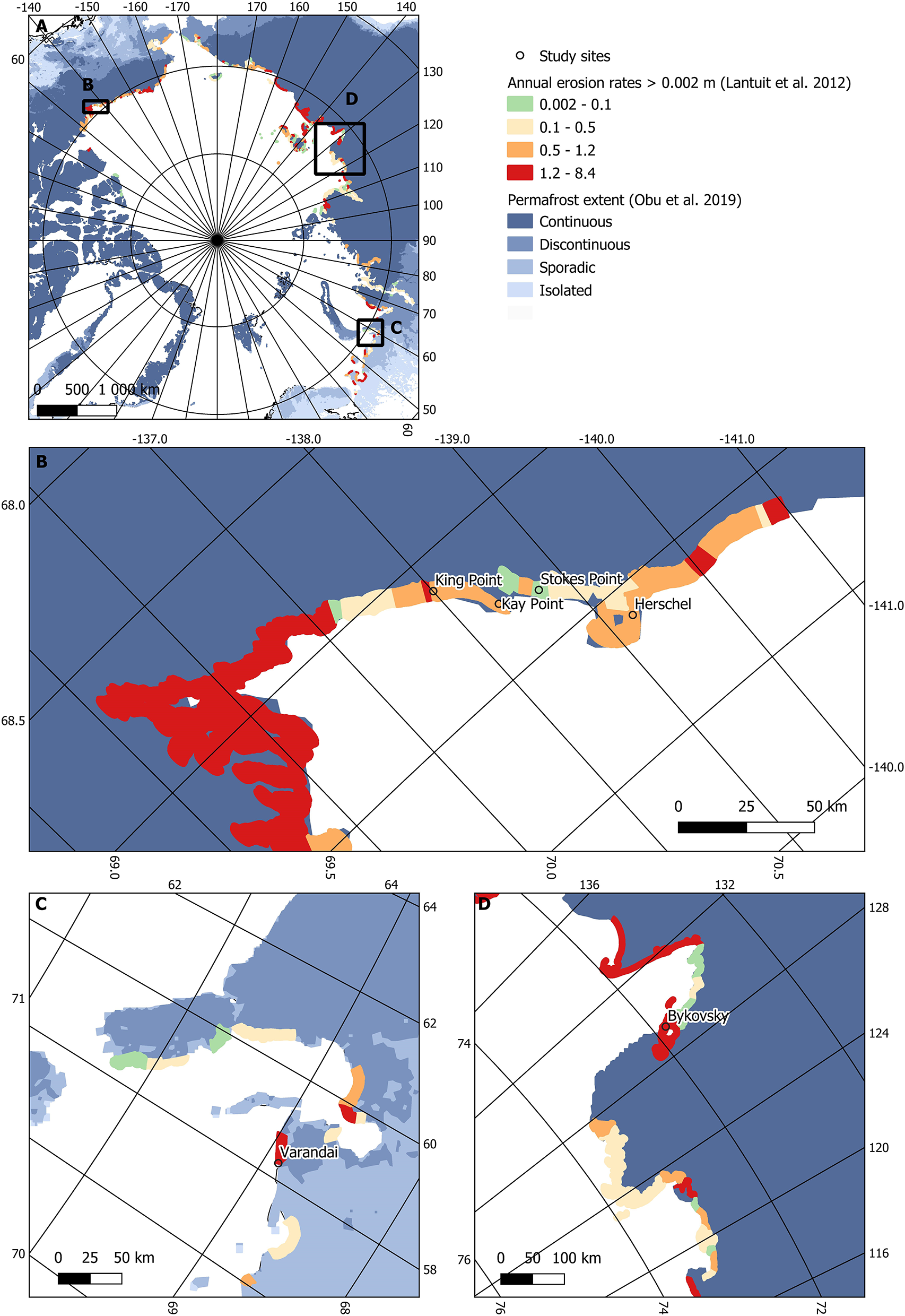
(A) Location of study areas, annual erosion rates (source: Lantuit et al., 2012) and permafrost zones (source: Obu et al., 2019b). (B) zoom for Beaufort Sea coast, (C) zoom for Barents Sea Coast, (D) zoom for Laptev Sea Coast.
Erosion dynamics in Arctic shorelines relate to cold climate and geomorphic impacts of permafrost, ground-ice, snow, and sea-ice. The evolution of coastal features occurs during the thawing and sea-ice-free seasons (Kroon, 2014). Depending on the morphology of the coastline and the ground ice content, thermo-abrasion (block failures) or thermo-denudation (retrogressive thaw slumps) are the main erosion processes (Lantuit, 2008; Hoque and Pollard, 2009). Coastal zones with horizontal thermo-erosional niches, especially when combined with large surface areas separated by ice wedges, are prone to block failures (Hoque and Pollard, 2004). The thermal-mechanical erosion undercuts the frozen cliff, and under the force of gravity, the heavy overhanging blocks of soil detaches from the coast (Lantuit, 2008). On average the erosion rate on Arctic coasts is 0.5 m/year, but in the Laptev East Siberian and the US and Canadian Beaufort Seas the rates are much higher (3 m/year and more) (Lantuit et al., 2012, see also Figure 1). The Barents Sea coast also includes low-gradient sandy shores with comparably high erosion rates (2–5 m/yr, Sinitsyn et al., 2020).
2.1.1. Canadian Beaufort (Yukon) Sea Coast
The approximately 280 km long Yukon Coast lies between the Alaskan border and the Mackenzie Delta in Canada, in the continuous permafrost zone. The climate has a continental character in winter and maritime influences in summer. Herschel Island is located approximately in its center. Komakuk Beach, around 40 km west of Herschel Island, is the closest weather station in this area (Obu et al., 2016). From 1971 to 2000 the mean air temperature was −11.3°C. The coldest temperatures were measured in February and the warmest in July, with averages of −25.3°C and 7.8°C, respectively (Government Canada, 2019). The coastal areas of the Beaufort Sea are typically ice-covered from October to June. From late August to September, storms become increasingly frequent and can generate significant high waves greater than 4 m (Solomon, 2005). Tides are in the order of 0.3 to 0.5 m in this region (Hequette et al., 1995). The coastal erosion processes mainly take place during this ice-free storm season (Obu et al., 2016).
In this area, low-relief landforms like beaches, barrier islands and spits, inundated tundra, tundra flats and slopes, and active cliffs are common (Irrgang et al., 2018). Around 33% of the coast shows active slumps, and 13% shows high bluffs with no slumping. Such slumps as well as bluffs exist, for example, on Herschel Island. A site with active slumps on the west coast (Avadlek as described in Obu et al., 2016) with a length of about 700 m and bluff heights of 10–25 m has been selected for analyses (Figure 2A). The slope orientation of the Avadlek site favors tests for the cliff-top detection approach as the majority of available satellite data is acquired by right looking system set ups and from ascending orbits (see Table 1).
Figure 2

Study sites along the Beaufort Sea Coast, Canada: (A) Avadlek on Herschel Island, (B) Kay Point, including shoreline points for rate calculations from Irrgang et al. (2017) and Landsat trend data based on probability of land to water change between 1999 and 2014 (Nitze et al., 2018) (visualization based on vectorized 30 × 30 m pixels). The baseline for rate calculations in this paper is shown in addition. Background: RGB (band 4, 3, and 2) composite of Sentinel-2 (optical, multi-spectral), Sep 20 2018.
Table 1
| Sensor (band, polarization, incidence angle range) | Region | Date | Nominal | Pass | Site specific |
|---|---|---|---|---|---|
| resolution [m] | incidence angle [°] | ||||
| PALSAR/ PALSAR-2 (L-band, HH, HV; 33–43°) | Herschel Island & Kay Point | 2007-08-31 | 12.5 | Ascending | 37.5 & 39 |
| 2008-09-02 | 12.5 | Ascending | 38 & 39.5 | ||
| 2017-07-26 | 10 | Ascending | 34.3 & 36 | ||
| 2018-07-25 | 10 | Ascending | 34.5 & 36 | ||
| Bykovsky Peninsula | 2007-09-04 | 12.5 | Ascending | 38 | |
| 2008-09-06 | 12.5 | Ascending | 38.5 | ||
| 2017-09-05 | 10 | Ascending | 40 | ||
| 2018-08-07 | 10 | Ascending | 40 | ||
| Varandai | 2007-08-01 | 12.5 | Ascending | 38 | |
| 2008-08-03 | 12.5 | Ascending | 38 | ||
| 2017-09-23 | 10 | Ascending | 41 | ||
| 2018-07-14 | 10 | Ascending | 41 | ||
| Sentinel-1 (C-band, VV, VH; 34–42.5°) | Herschel Island & Kay Point | 2017-07-15 | 10 | Ascending | 40 & 40.5 |
| 2018-07-22 | 10 | Ascending | 40 & 40.5 | ||
| 2017-07-29 | 10 | Descending | 43.2 &40.2 | ||
| 2018-07-24 | 10 | Descending | 43.2 &40.2 | ||
| Bykovsky Peninsula | 2017-07-25* | 10 | Descending | 39.8 | |
| 2018-07-20* | 10 | Descending | 39.8 | ||
| Varandai | 2017-07-28 | 10 | Descending | 38 | |
| 2018-07-23 | 10 | Descending | 38 | ||
| TerraSAR-X (X-band, HH; 19–53°) | King Point | 2018-06-15* | 0.62 | Descending | 51 |
| 2018-07-07* | 0.62 | Descending | 51 | ||
| Kay Point | 2018-07-13 | 0.69 | Ascending | 40 | |
| 2019-01-27 | 0.69 | Ascending | 40 | ||
| 2018-08-12* | 1.35 | Descending | 19.5 | ||
| Stokes Point | 2018-07-16* | 0.96 | Descending | 29.5 |
List of available Synthetic Aperture Radar acquisitions grouped by sensor and study area.
indicates use for incidence angle and landcover analyses only.
In 2006 around 78% of the Yukon coastline, including Herschel Island, was affected by coastal erosion processes (Obu et al., 2016). Excluding Herschel Island, the mean annual rate of shoreline change from 1950 to 2011 was −0.7± 0.2 m/year. The highest erosion rates were measured at shorelines characterized by spits (Irrgang et al., 2018) and capes. One example is Kay Point (Figure 2B). It includes a NE facing coastline stretch of approximately 2km length characterized by approximately 4 m high bluffs, but no thaw slumps. This coast segment has been selected for analyses, since it is a long-term monitoring site of the Geological Survey of Canada (Forbes et al., 1995, site 5280), as well as due to satellite data availability (Table 1), specifically very high spatial resolution SAR, which allows investigation of radar shadow occurrence. Reference erosion rates with geospatial information is available from Irrgang et al. (2017) for this region. Both sites (Avadlek on Herschel Island and Kay Point) are located in areas with comparably high Soil Organic Carbon (SOC) mobilization (Couture et al., 2018).
2.1.2. Bykovsky Peninsula, Laptev Sea Coast
The Bykovsky peninsula is located southeast of the Lena Delta in northeastern Siberia, and lies within the zone of continuous permafrost. The weather has an almost continental character, although it is surrounded by the Laptev sea (Lantuit et al., 2011). The mean annual temperature is −11.5°C with long harsh winters and short cold summers. The open water season is between July and September, but can begin as early as late May (Lantuit et al., 2011; Günther et al., 2013). The length of the open water season at the Laptev Sea Coast has a strong influence on annual rates and is conditioned by the Arctic Oscillation in winter and summer (Nielsen et al., 2020). Concurrent with the open water season, the highest storm activity takes place in these months (Lantuit et al., 2011). Storms are in general the largest driver of erosion in the Arctic, and therefore the coastal erosion is mostly limited to the open water season in July to September. However, even during this period chunks of sea ice can reduce the wave activity (Lantuit, 2008).
The relief of the peninsula is dominated by flat elevated areas up to 40 m above sea level and thermokarst depressions near sea level (Grosse et al., 2005). At the over 150 km long shoreline, various coastal landforms exist, such as sandbars, lagoon barriers, ice complex cliffs, thermokarst basins (alases), and thaw slump coasts according to Lantuit et al. (2011). Between 1951 and 2006, alases and retrogressive thaw slumps underwent erosion at a rate of 1.02 and 0.91 m/year, respectively (Lantuit et al., 2011). These rates are significantly higher than the other coast types on the Bykovsky Peninsula, which underwent erosion at rates between 0.40 and 0.47 m/year (Lantuit et al., 2011). A three kilometer long stretch along the west coast, which is characterized by retrogressive thaw slumps has been selected for this study (Figure 3A). Similarly to the Herschel Island site, the slope orientation favors testing the cliff-top detection approach.
Figure 3
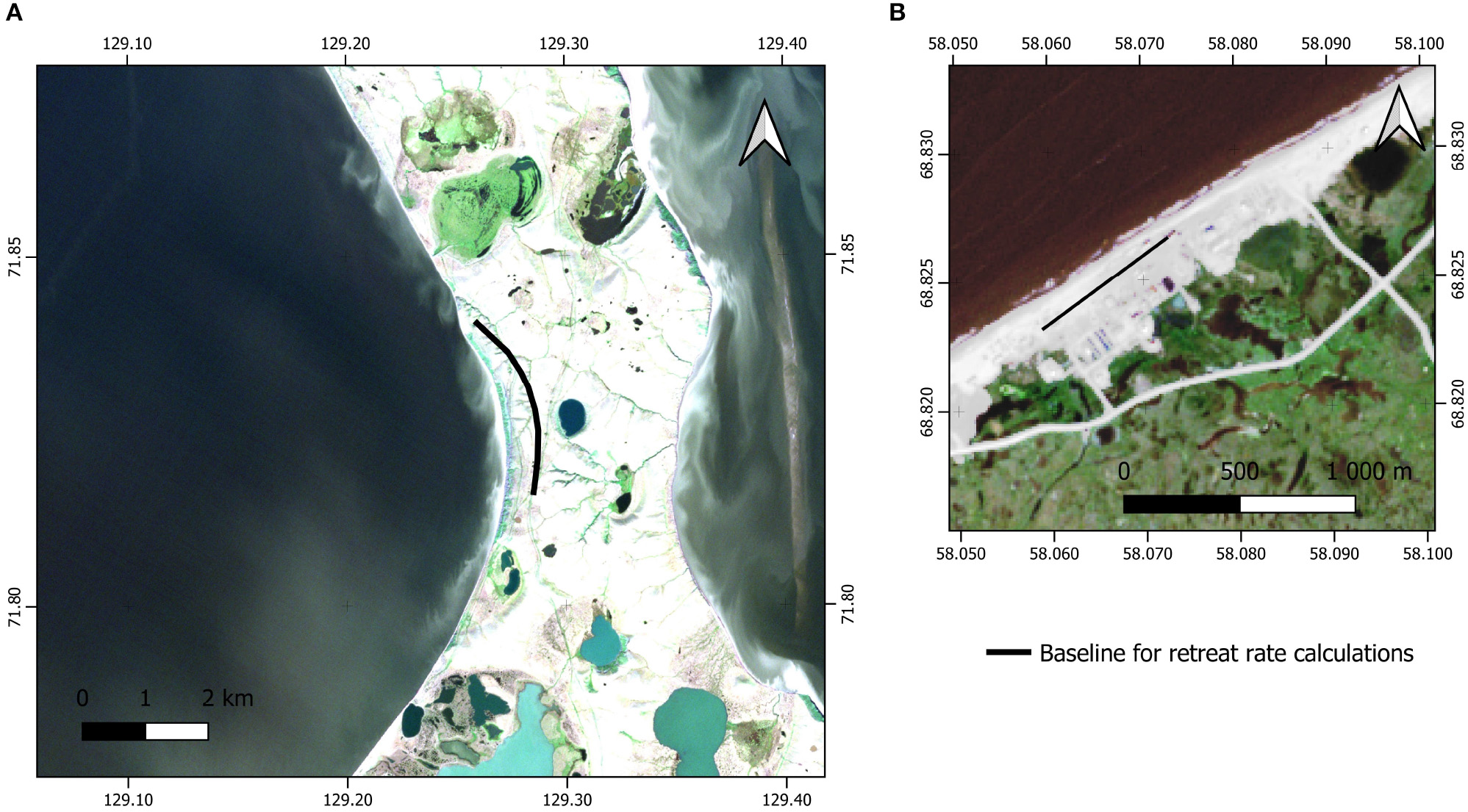
Russian study sites: (A) West coast of the Bykovsky Peninsula, (B) Varandai, Barents Sea Coast. The baseline for rate calculations in this paper is shown in addition. Background: RGB (band 4, 3, and 2) composite of Sentinel-2 (optical, multi-spectral), Aug 28 2018 and Aug 8 2019.
2.1.3. Varandai, Barents Sea Coast
The study region at the Barents sea coast in the northwest of Russia is warmer regarding ground and air temperatures than the other sites. It lies in the zone of sporadic to discontinuous permafrost (Figure 1). Le et al. (2018) report a mean annual air temperature between −3.8 and −4.8°C in 2012–2014. The coldest air temperature of −39.4°C was measured in January, and the warmest, 30°C, in July. Storm surges with magnitudes of 1.5–2 m, and tides with high amplitudes of 0.5 m are common (Leont'yev, 2003).
In general, the landscape varies from wide, low-gradient sandy shores with dune belts to sub-vertical ice-rich bluffs and narrow beaches (Guégan and Christiansen, 2016). The coast is formed by a marine terrace 2 to 6 km wide, and the sediment body is predominantly sand. The coastal cliffs, where present, are mostly between 3 and 10 m high. Thermal erosion only occurs locally, and does not play a large role in the coastal dynamics. Coastal erosion rates of 1 to 4 m/year are common (Leont'yev, 2003). This applies to specifically the area near Varandai, which has been selected as example for low relief coast with an extensive sandy beach area (approximately 700 m, Figure 3B). Sinitsyn et al. (2020) report on average −1.8 m/year from 1951 to 2013 in the proximity. Several buildings have been destroyed between 2004 and 2012. This period included a storm surge which occurred in summer 2010.
2.2. Synthetic Aperture Radar Data
Three different wavelengths from SAR sensors from four different satellite missions have been investigated. This also included the analyses of different polarization combinations. The choice of acquisition dates and wavelengths was determined by data availability. A further issue is also spatial resolution. Although a long history of C- and L-band SAR acquisition exists, older platforms such as ERS-1/2 (European remote sensing satellites 1 and 2, 1991–2011) or JERS-1 (Japanese Earth Resources Satellite 1) offer only comparably coarse spatial resolution (about 30 and 18 m, respectively) and limited polarization combinations. Open access and continuous acquisitions only exist for C-band (Sentinel-1 Copernicus mission). X-band and L-band availability and access is in general limited. Table 1 provides an overview of used sensors, their specifications and dates. Recent annual erosion rates were determined for 2017 to 2018 using L-band and C-band data and for part of the open water season of 2018 in case of X-band data. A longer time period (decadal time scale) could be only investigated for L-band as only in this case consecutive missions with similar acquisition properties are existing. The years 2007 and 2008 have been therefore analyzed for L-band in addition to 2017 and 2018. The actual dates varied from sensor to sensor also due to acquisition strategies, revisit intervals and image quality. The availability of polarization combinations also varies across the sensors. At maximum two types of combinations have been available for the study sites, including HH (horizontally sent and horizontally received), VV (vertically sent and vertically received) as well as HV and VH.
The Phased Array type L-band Synthetic Aperture Radar (PALSAR) and PALSAR-2 are L-band SARs with a center frequency around 1.2 GHz (JAXA, 2008, 2018). They are follow-on missions of JERS-1. PALSAR was launched on board the Advanced Land Observation Satellite (ALOS) in January 2006 and sent information until its failure in April 2011. ALOS was replaced in May 2014 by ALOS-2, carrying the PALSAR-2. Both satellites have a sun-synchronous, sub-recurrent orbit, but the 14-day revisit time of ALOS-2 is much shorter than the ALOS revisit time of 46 days (Shimada, 2009; JAXA, 2018). Due to their duration and orbits, the PALSAR datasets are suitable for long-term studies of the Arctic. Two sets of data were used from the PALSAR satellites. First, PALSAR Fine Beam (FB) dual polarization images with 12.5 m nominal resolution in HH and HV polarizations were analyzed. Second, PALSAR-2 Stripmap mode 3 (SM3) images with 10 m nominal resolution, also in HH and HV polarizations, were investigated. In total four images with the same orbit, one image per year, for each area of interest were used.
The Sentinel-1 mission is part of the European Union's Copernicus program. The mission consists currently of two satellites with a near-polar, sun-synchronous orbit, 180 degrees apart from each other. The two earth observation satellites Sentinel-1A (launched in April 2014) and Sentinel-1B (launched in April 2016) have an identical C-band SAR sensor on board (Schubert et al., 2017). The Interferometric Wide Swath (IW) mode combines a swath width of 250 km with a medium-high ground resolution of 5 × 20 m. Products in ground range are distributed with 10 m nominal resolution. The incidence angle range is potentially 31° to 46°. Images can be captured in dual polarization (HH+HV or VV+VH). Only VV+VH is available for the study areas for this mode and resolution. Like the PALSAR/PALSAR-2 data sets, one image per year with the same relative orbit for every area of interest was analyzed. The years 2017 and 2018 were chosen to enable the comparison of the coastal erosion rates with the PALSAR/PALSAR-2 images. Images with ascending and descending pass directions were available for the Canadian Beaufort Sea Coast, and both were used for this study.
TerraSAR-X was launched in June 2007, and is a commercial German X-band SAR earth observation satellite. It has a sun-synchronous orbit and a repeat period of 11 days. The standard operational mode is the single receive antenna mode, which can be used in three different modes: SpotLight (SL), StripMap (SM) and ScanSAR (SC). The SpotLight mode uses phased array beam steering in azimuth direction to increase the illumination time. It can further be divided in the High Resolution SpotLight (HS) and Staring SpotLight (ST) mode. The ST scene size and resolution is highly dependent on the incidence angle, because the antenna footprint depends on the scene, and the scene length corresponds to the length of the antenna footprint. The Spotlight mode achieves an azimuth resolution up to 0.24 m. For this mode only single polarization acquisitions are available (HH). In this study TerraSAR-X images in ST mode with incidence angles between 19° and 51° as well as ascending and descending acquisitions are available for parts of the Beaufort Sea Coast (Kay point, King Point and Stokes Point). The incidence angle impacts the spatial resolution. The applied nominal resolution for the used images therefore ranges from 0.62 to 1.35 m (see Table 1). The only image pair which allows for time series analyses has an ascending pass designation and covers only Kay Point. In addition, the second acquisition is from winter time which may affect the classification results (accuracy) as well as annual rates (disproportional representation of thaw period).
The PALSAR/PALSAR-2 L-band and Sentinel-1 C-band data sets used in this study were recorded in the most likely open water months, from June to September. This time frame was chosen to take advantage of the backscatter difference between land and water, which is greater than the difference between land and sea ice. The high-resolution TerraSAR-X X-band data sets were available for June, July, August and October 2018 and January 2019. For calibration, only data from the sea ice free season/areas were used. Table 1 summarizes the used acquisitions.
The availability of ascending and descending image pairs by L-band and C-band data allows the comparison of cliff-top classification based results and land-water boundary based results for the Herschel site. C-band was found not applicable for Bykovsky, due to constant high wave action in the proximity. Therefore only L-band has been investigated at this site.
Data from all three bands are available at the Kay Point site only. Continuous stretches of steep cliffs facing the sensor are not present in acquisitions for this area. Therefore only the land-water boundary is investigated. A specific feature in this area is the occurrence of radar shadows in X-band where the bluffs are steep and face away from the sensor, due to the comparably high spatial resolution. The land-water boundary only is also investigated in case of Varandai; here due to the absence of steep coast.
2.3. Auxiliary Multi-Spectral Data and Derived Products
A landcover classification provided by Bartsch et al. (2019b) was used to define the coastline and to calculate the coastline orientation with respect to the sensor. This classification is based on a combined approach of supervised and unsupervised classification using SAR (Sentinel-1 VV, IW mode) and multi-spectral data (Sentinel-2). Sentinel-2 is an European mission to deploy wide-swath, high-resolution, multi-spectral observation satellites. It deployed two twin satellites, Sentinel-2A and -2B, in a sun-synchronous orbit 180° apart from each other. Sentinel-2A was launched in June 2015 and Sentinel-2B in March 2017. The optical sensor samples 13 spectral bands. The spatial resolution depends on the used band: four bands have a spatial resolution of 10 m, six bands of 20 m, and three bands of 60 m (ESA, 2015). Bands 3 (green, 10 m resolution), 4 (red, 10 m), 8 (near infrared, 10 m), 11 (SWIR, 20 m), and 12 (SWIR, 20 m) from July/August 2015–2018 have been used for the classification (Bartsch et al., 2019a,b).
Sentinel-2 images are further used for visualization purposes as well as to aid validation and calibration sample selection. True color RGB composites (band 4, 3, and 2) with a spatial resolution of 10 m have been prepared. The images were acquired on Jun 14, Jul 23, Sep 20 2018 (Beaufort Sea Coast), Aug 28 2018 (Bykovsky Peninsula), and Aug 8 2019 (Varandai).
A Landsat-derived product was used for the assessment of the SAR retrievals. Data from this mission are commonly used for change detection and Arctic landcover classification (Bartsch et al., 2016). NASA's Landsat mission deployed a series of land observation satellites. Landsat 5, 7, and 8 were launched in 1984, 1999, and 2013, respectively. They provide visible-, and infrared–wavelength images of all land and near-coast areas on Earth in 30 m spatial resolution. Landsat 7 and 8 have additional thermal bands in 60 m resolution and a panchromatic band in 15 m resolution. These datasets formed the basis for trend analyses described in Nitze et al. (2017, 2018). Trends from various multi-spectral indices in combination with the random forest machine-learning algorithm allow the retrieval of land surface change probabilities. They have been already applied for land-water change for lakes (Nitze et al., 2017, 2018). Resulting products are available open access (Nitze, 2018) for selected Arctic regions at 30 m spatial resolution spanning 1999–2014. For this study, we expanded the dataset extent along the Beaufort Sea Coast to Herschel and Kay Point, which were not covered in previous analyses.
2.4. Pre-processing of SAR Data
The Sentinel-1, PALSAR-2, and TerraSAR-X data were preprocessed in ESA's SNAP toolbox (ESA, 2019b). The PALSAR data was processed in the ASF MapReady software (ASF, 2019).
Pre-processing included radiometric calibration as well as multi-looking in case of the PALSAR-2 and TerraSAR-X images (1:4 and 1:2, respectively, range:azimuth), since the data were available as single-look complex images. This step was not necessary for the Sentinel-1 data, because Ground Range Detected (GRD) products were used. GRD products are detected, multi-looked, and projected to ground range using an Earth ellipsoid model (ESA, 2012).
To reduce speckle, a filtering step was added. The Lee Sigma filter was applied (sigma = 0.9, window = 7 × 7, and target window size = 3 × 3). This filter assumes that 95.5% of the pixels are distributed within the two-sigma range from its mean. It replaces the center pixel of a scanning window with the average of those pixels within the two-sigma range of the center pixel. Pixels outside the two-sigma range are not included into the sample mean computing, and a speckle reduction is achieved (Lee et al., 2009).
The third step was ellipsoid correction of the data (as suggested in Stettner et al., 2017). For areas of continuous erosion a terrain correction cannot be applied, when a precise Digital Elevation Model (DEM) for the constantly changing coastline area is not available. Therefore only images with the same orbit constellation are comparable to each other. These steps were carried out with the SNAP (Sentinel Application Platform) toolbox provided by the European Space Agency and the scattering coefficient σ0 was derived. During the ellipsoid correction, the local incidence angle (based on ellipsoid) was extracted. The final step involved converting σ0 to decibels. The resulting nominal resolution is provided in Table 1.
In case of PALSAR data, ellipsoid correction was carried out first in the ASF MapReady software, and afterwards the Lee Sigma filter was applied in the SNAP toolbox.
2.5. Identification of Steep Coasts Facing the Sensor
Samples for calibration and validation are required for all three target classes: water, land and steep coasts facing the sensor. Water and land reference data are available through the existing land cover classifications and the Sentinel-2 images. Steep coasts can be also partially identified with Sentinel-2 (visible thaw slumps), but they are only of relevance when they are facing the sensor.
Steep coasts that are facing the sensor have a relatively high backscatter coefficient. This is mainly caused by the foreshortening effect and occurs only when the cliff faces the sensor. Therefore it is important for the threshold determination proposed by Stettner et al. (2017) to consider the orientation of the coast relative to the incoming signal.
Calculating the coastline orientation means calculating the intersection angle between the coastline and the line of sight (LOS) of the sensor. For threshold determination, the coastline of the Beaufort Sea coast was extracted from a land cover classification provided by Bartsch et al. (2019b) and divided into segments. The raster (20 × 20 m) was vectorized, the land water boundary vector manually extracted and simplified using the Douglas-Peucker algorithm (Douglas and Peucker, 1973) with a smoothing distance of 30 m. The resulting vector was split at every second vertex to create the segments. The coordinates of each segment's midpoint and endpoints were then derived.
The midpoints were moved 40 m toward the satellite to test whether the coast was facing toward or away from the satellite. The moved point lies outside the land area (over the ocean) if the coastline faces the satellite and inside (over the land surface) if it faces away.
Finally the angle between the LOS of the sensor and the coast segment was calculated. The gradient of the LOS, m2, was derived from the inclination of the satellite's orbit. The angle α was calculated
where m1 is the gradient of the coast segment. This gradient is calculated based on the start and end point of the respective line vector. Results served for choice of analyses segments, including calibration sites for the classification threshold determination as well as for erosion rate retrieval.
2.6. Threshold Determination and Classification
In general, we followed the approach by Stettner et al. (2017) but extended it in order to consider local incidence angle dependencies as necessary for transferability of the approach. Also the case for land-water boundary detection as an alternative is included. A threshold method which considers three surface types (water, land and steep cliff) as well as incidence angles is required. The assumption is that thresholds differ for each sensor type/ wavelength. Ellipsoid derived incidence angles can be assumed to be of limited applicability for local incidence estimation at steep cliffs (are in general smaller at cliffs facing the sensor), but are nevertheless treated similarly to the other classes and are discussed.
Radar shadow needs to be taken into consideration as a fourth class in case of the TerraSAR-X staring spotlight mode images, due to their high spatial resolution (less than 1 m). Radar shadow occurs at cliffs facing away from the sensor resulting in an about five meter wide affected area at Kay Point. This effect is always present at this viewing geometry which allows utilization of data from winter acquisitions. Figure 4A shows an example of a summer and a winter image. The determined backscatter for radar shadow is in the same order as for smooth water surfaces (appr. −20 dB, Figure 4B). The backscatter characteristics for open water (threshold function separating open water from land) are therefore also used for application during winter in case of the selected coastal stretch at Kay Point. The example also includes typical values for cliffs collected from the W and NW facing parts of the Babbage Estuary, which is located SW from Kay Point within the TerraSAR-X scene extent. They demonstrate that thresholds separating cliffs from the “land” class determined from summer images are not applicable for the category cliffs facing to the sensor in winter (exposed soils are wet and therefore exhibit a strong frozen-unfrozen difference), but all cliffs at the selected coastal segment at Kay Point are facing away from the sensor.
Figure 4
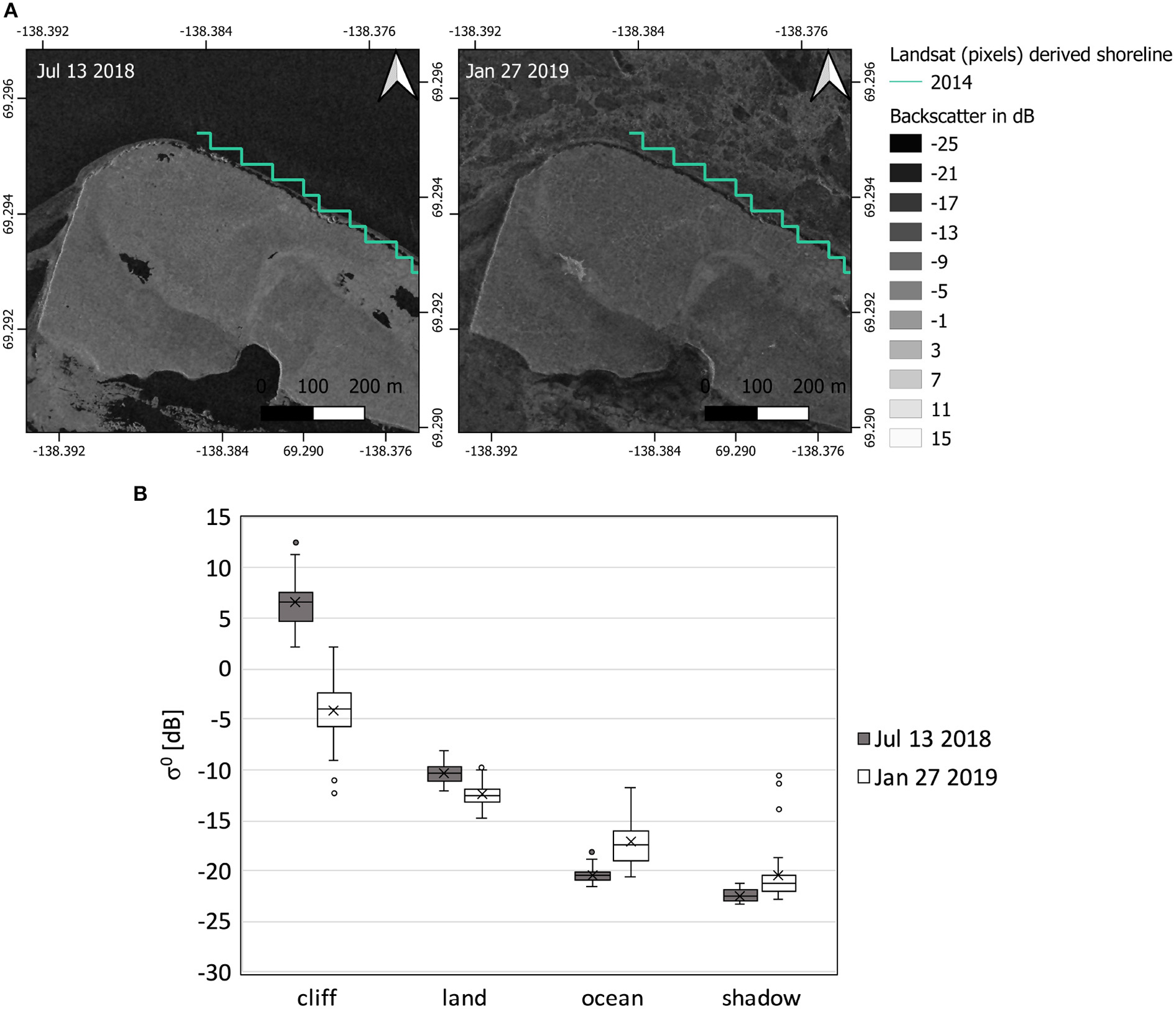
Backscatter characteristics (σ0 in dB) of TerraSAR-X at Kay Point: (A) Example of a summer and a winter acquisition including the Landsat derived coastline for demarcation of the analysed coast segment (using) trend data based on probability of land to water change between 1999 and 2014 (Nitze et al., 2018); visualization based on vectorized 30 × 30 m pixels), (B) boxplots of backscatter samples for all relevant classes (cliffs facing toward the sensor, land, ocean, and radar shadow) at 40 degree incidence angle for summer and winter.
Samples were taken to analyze the dependence of σ0 on incidence angle for each of the three surface classes. The samples were manually selected using the auxiliary datasets. The landcover classification from Bartsch et al. (2019b) was used to identify sample locations for land and water areas. Potential areas with steep cliffs facing the sensor have been identified supported by the coast orientation dataset which was created in the preceding step. The incidence angle range was different for each satellite. The PALSAR/PALSAR-2 range varied from 33° to 43°, Sentinel-1 from 34° to 42.5°, and TerraSAR-X from 19° to 51°. Nearly all images were used (except January acquisition from TerraSAR-X), and samples that cover the maximum possible incidence angle range were selected. This required the use of data from two additional sites with differing viewing geometry (King Point, 20 km south of Kay Point and Stokes Point, 20 km to the North) in case of TerraSAR-X. Regions with sea-ice were excluded from the water class sampling. The sample sets were grouped by satellite, surface class, and polarization. Each group was divided into a training set (to calculate the threshold function) and a testing set (to test the quality of the classification results). The separation was made based on the rasterized training polygons. Every second pixel in the sequence (row by row) was excluded from the training and used for validation later on. The sample sizes of the three classes reflect approximately the occurrence in the images. The sample size (area covered) of steep cliff features is therefore much smaller than for the other classes (less than 1% of the complete sample dataset). Approximately 15–17% for land and 83–84% for water are contained in the sample datasets for each of the wavelengths. The sample dataset covers in total about 617 km2.
In order to classify the images, a functional relationship between σ0 and the incidence angle θ was calculated following a similar approach as suggested by Bartsch et al. (2017) but applying a linear function as only a limited range is used (see also Widhalm et al., 2018; Bartsch et al., 2020; with a being the slope and b the intercept).
In general, the water samples show the lowest backscatter values, and the coast samples the highest (example for X-band, see Figure 4). For this reason threshold functions were calculated to differentiate the water from land and land from steep cliffs (but not water from steep cliffs). The parameters a and b have been derived for each wavelength and polarization combination separately. The standard deviation for the different landcover types are also expected to differ. To derive more precise threshold functions, the standard deviation of the absolute residuals was therefore considered (Table 2). The threshold between water and land was calculated as:
where and are the function fitted to the water and land samples and their standard deviations are stdwater and stdland. Similarly, the threshold function between the land and steep cliff classes was calculated as:
where is the function fitted to the land samples and its standard deviation is stdcliff.
Table 2
| Sensor | Polarization | Water | Land | Cliff |
|---|---|---|---|---|
| PALSAR | HH | 0.69 | 0.76 | 0.96 |
| HV | 0.56 | 0.45 | 0.75 | |
| PALSAR-2 | HH | 0.64 | 0.87 | 1.36 |
| HV | 0.59 | 1.31 | 0.83 | |
| Sentinel 1 | VH | 0.92 | 0.81 | 0.69 |
| VV | 1.88 | 0.77 | 0.78 | |
| TerraSAR-X | HH | 1.44 | 0.78 | 1.36 |
Standard deviation of absolute residuals for water, land and cliff for each satellite and polarization (σ0 in dB) for use in equation 3 and 4.
These threshold functions were used to classify the image pixels. During the classification process it was calculated whether the σ0 pixel values lie below or above the threshold functions. If the σ0 pixel value was below the σw/l threshold it was classified as water. Otherwise, it was tested whether the σ0 values lie below or above the σl/c threshold. Every pixel above the threshold was classified as steep cliff, every value below as land.
The error evaluation was carried out separately for the different polarizations. The “producer's accuracy” and the “user's accuracy” have been derived.
The classification results were then used to derive vectors representing the land-water boundaries and cliff-land boundaries, respectively. The classification raster was vectorized and then all vectors, which represent such boundaries within the areas of interest manually extracted. These vectors were then split perpendicular to the relevant baseline (at their end and start point, see Figures 2, 3 for baseline locations) for the erosion rate calculation.
2.7. Post-processing of the Landsat Landsurface Trend Products
Probabilities of erosion and accretion (change of land to water and visa versa) as well as no change are available for the time period 1999–2014. Samples of probabilities have been taken for published coastline positions at Kay Point for 1950, 1990, and 2011 [Irrgang et al. (2017), see Figure 5]. The extracted values (mean and median) indicate that a probability threshold between 0.4 and 0.6 could be applicable for retrieval of land to water conversion. Probabilities drop sharply in front of the NE oriented coastal erosion area at Kay Point (Figure 6, left). Differences between thresholds of 0.45, 0.5, and 0.55 are small (Figure 6, right). A probability threshold of 0.5 has been therefore selected based on these samples in order to derive potential areas of erosion at the Beaufort Sea Coast sites and at the Bykovsky peninsula. The resulting raster has been vectorized along the selected coastal segments and segments selected as for the SAR classification results (see section 2.6).
Figure 5
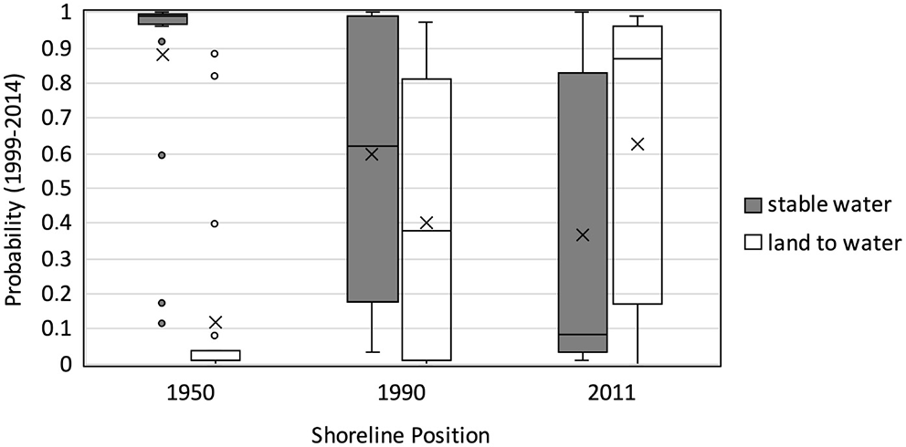
Probabilities for stable water and land to water conversion derived from Landsat (1999–2014) for shore line positions 1950, 1990, and 2011 at Kay Point (source Irrgang et al., 2017, see also Figure 2B).
Figure 6
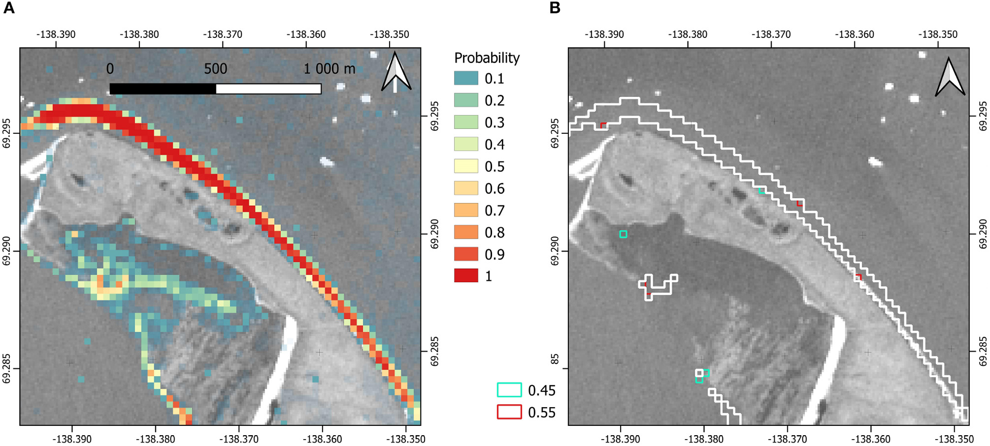
Probabilities for land to water conversion derived from Landsat (1999–2014) at Kay Point (see also Figure 2B). (A) overlay of probabilities for each pixel, (B) vectorized classifications for >0.5 (white), >0.45 (blue), and >0.55 (red). Background: Band 2 (blue) of Sentinel-2 Sep 20 2018.
2.8. Erosion Rate Estimation
In line with Stettner et al. (2017) the Digital Shoreline Analysis System (DSAS), an ArcGIS extension provided by the United States Geological Survey (Himmelstoss et al., 2018), was used to derive the coastline erosion rates. DSAS calculates rate-of-change statistics for a chronological series of shoreline vectors. For the erosion rate calculation, baselines and transects were defined. Considering the spatial resolution, a transect distance of 10 m was used for the PALSAR/PALSAR-2 and Sentinel-1 shorelines, and a distance of 1 m was used for the TerraSAR-X shorelines. The shoreline uncertainty values (unc) were chosen to be equal to the spatial resolution of the image (PALSAR 12.5 m, Sentinel-1 10 m, PALSAR-2 6.8–8.2 m, and TerraSAR-X 0.69 m).
Three statistics and their uncertainty were calculated: the net shoreline movement (NSM), the end point rate (EPR), and the weighted linear regression (WLR). For the WLR calculation, shorelines from three or more dates are necessary.
The NSM is the distance in meters between the oldest and the most recent shoreline positions for each transect. This NSM value was used to determine the EPR and the associated uncertainty as documented in Himmelstoss et al. (2018).
The WLR was calculated by using least-squares regression to fit a line through the transect points. Data points with a small spatial uncertainty, were given more weight (Himmelstoss et al., 2018). Like the EPR, the WLR expresses a shoreline change rate for each transect. The EPR is the change between pairs of sequential observations, and the WLR is the overall trend.
The WLR could only be calculated for the PALSAR/PALSAR-2 shoreline time series because the other datasets only have two timepoints. The NSM and EPR were calculated for the Sentinel-1 and TerraSAR-X data sets. The 2017–2018 EPR for the PALSAR/PALSAR-2 coastlines that overlap with the Sentinel-1 data set were calculated for comparison.
3. Results
3.1. Threshold Functions for Classification
The standard deviation of backscatter for water is highest for C- and X-band, which reflects wave action and the comparably short radar wavelength with respect to wave height. Deviations are in general high for all steep sensor facing cliffs as affected areas are comparably small (mixed pixels) and topography varies locally. The standard deviation is below 1 dB in most cases with exceptions not exceeding 2dB. Table 3 summarizes the parameters of the threshold functions grouped by satellite and polarization. A slope (a) close to zero indicates low incidence angle dependence. This is the case for the cliff-land threshold in case of C- and X-band for all tested polarizations due to low dependence of the land and cliff class. The same applies to the land-water boundary for X-band. In all other cases, including all L-band polarizations (Figure 7), the incidence angle needs to be considered for the threshold determination, which is in general driven by the properties of water surfaces in case of C- and X-band.
Table 3
| Sensor | Polarization | Threshold | a | b |
|---|---|---|---|---|
| PALSAR-2 | HH | Cliff–Land | -0.203 | 4.353 |
| Land–Water | -0.382 | -0.620 | ||
| HV | Cliff–Land | -0.245 | -4.467 | |
| Land–Water | -0.203 | -18.753 | ||
| Sentinel-1 | VH | Cliff–Land | -0.055 | -9.898 |
| Land–Water | -0.220 | -13.224 | ||
| VV | Cliff–Land | 0.059 | -7.266 | |
| Land–Water | -0.303 | -3.070 | ||
| TerraSAR-X | HH | Cliff–Land | -0.023 | -2.029 |
| Land–Water | -1.041 10−4 | -15.73 |
Threshold parameters for each satellite and polarization.
The parameters a and b refer to Equation (2). PALSAR is omitted because its images were classified based on the PALSAR-2 threshold.
Figure 7
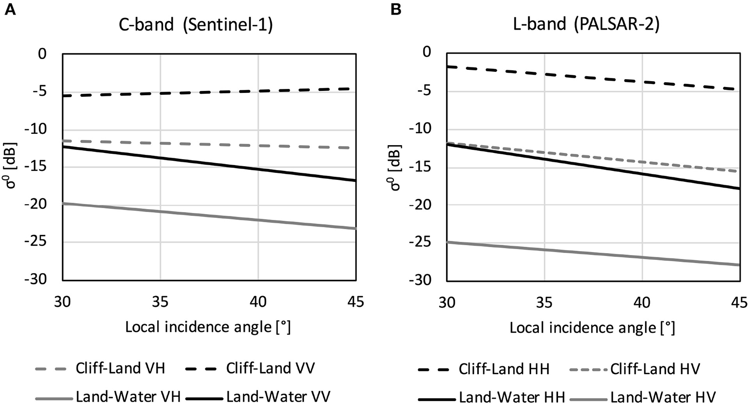
Threshold functions derived for (A) C-band (Sentinel-1, Interferometric Wide Swath mode) and (B) L-band (PALSAR-2, Fine Beam mode). Local incidence angles (x-axis) are derived with respect to the ellipsoid. For equation parameters see Table 3.
The Sentinel-1 VV polarized samples show higher backscatter values than the VH polarized samples, which is reflected in the threshold functions in Figure 7. The same applies to L-HH compared to L-HV. The PALSAR-2 samples were eventually used to calculate the threshold functions for both PALSAR and PALSAR-2, because of the wider incidence angle range available from the PALSAR-2 data.
3.2. Classification Accuracy
The threshold based classification results show the highest classification accuracy for co-polarized acquisition (Table 4). This can be shown for L-band as well as C-band.
Table 4
| Classified data | Reference data | Users accuracy | |||
|---|---|---|---|---|---|
| Cliff | Land | Water | |||
| PALSAR/PALSAR 2 HH | Cliff | 100 | 0 | 0 | 100.00 |
| Land | 0 | 71.51 | 0.3 | 93.70 | |
| Water | 0 | 28.49 | 99.7 | 97.43 | |
| PALSAR/PALSAR 2 HV | Cliff | 100 | 0.03 | 0 | 88.34 |
| Land | 0 | 77.14 | 14.14 | 52.76 | |
| Water | 0 | 22.83 | 85.86 | 94.84 | |
| Sentinel-1 VV | Cliff | 100 | 0.13 | 0 | 18.39 |
| Land | 0 | 97.56 | 4.13 | 78.47 | |
| Water | 0 | 2.31 | 95.87 | 99.63 | |
| Sentinel-1 VH | Cliff | 100 | 0.43 | 0 | 7.32 |
| Land | 0 | 66.34 | 0 | 100 | |
| Water | 0 | 33.23 | 100 | 95.13 | |
| TerraSAR-X HH | Cliff | 100 | 0 | 0 | 100 |
| Land | 0 | 99.87 | 0.6 | 97.41 | |
| Water | 0 | 0.13 | 99.4 | 99.97 | |
User's and producers accuracy of landcover classifications.
“Cliff” refers to steep coasts facing the sensor. Producer's accuracy values are highlighted in bold. All values are in %.
The producer's accuracy of the cliff classification is 100% for every polarization. In other words, all cliff samples were correctly classified as cliff, regardless of sensor. This is especially important for assessing coastal erosion based on cliff-top lines derived from steep sensor-facing coast classifications.
The Sentinel 1 user's accuracy values in case of the cliff class (areas with foreshortening), ranging from 7 to 18%, are relatively low. Independent from the polarization, only land samples were misclassified as cliffs. TerraSAR-X user's accuracy is also 100%. The area covered by the acquisitions is comparably small and does not include any mountain ranges. Water–land misclassification occurs for all sensors and polarizations due to wave action. The magnitude can be expected to vary with meteorological conditions and therefore results cannot be generalized.
3.3. Coastal Change Rates
All of the results show erosion, which indicates that the selected areas were predominately eroding as expected (Table 5). The calculated rates for the same regions based on images from different sensors are mostly in the same order of magnitude. Values range mostly between 3 and 9 m/year. Uncertainty values reflect the impact of spatial resolution and time interval. Values are small (less than one meter) for TerraSAR-X and comparably low for PALSAR/PALSAR-2 retrievals for 2007–2018 (0.4–4.3m) compared to annual changes (mostly more than 10 m).
Table 5
| Region | Sensor | Coastline | Years | Mean | Ref. | Ref. | Refernces |
|---|---|---|---|---|---|---|---|
| Type | Change | Change | Years | ||||
| Rate | Rate | ||||||
| m/year | m/year | ||||||
| Herschel Island, Avadlek | P., P.-2 | Cliff-Top | 07–08 | -9.68 ± 17.53 | |||
| P., P.-2 | Land–Water | 07–08 | -45.06± 17.53 | ||||
| P., P.-2 | Cliff-Top | 07–18 | -3.42 ± 4.32 | -6.8 ± 8.6 | 2012-2013 | Obu et al., 2016 | |
| P., P.-2 | Land–Water | 07–18 | -7.02 ± 2.65 | ||||
| P.-2 | Cliff–Top | 17–18 | -2.61± 14.83 | ||||
| P.-2 | Land–Water | 17–18 | -9.52 ± 11.2 | ||||
| S.-1 | Cliff–Top | 17–18 | -0.9 ± 8.01 | ||||
| S.-1 Asc. | Land–Water | 17–18 | -3.26 ± 13.88 | ||||
| S.-1 Desc. | Land–Water | 17–18 | -27.63 ± 14.34 | ||||
| Landsat | Land–Water | 99–14 | -4.19 ± 2.8 | ||||
| Kay Point East Coast | P. | Land–Water | 07–08 | -14.51 ± 8.77 | |||
| P., P.-2 | Land–Water | 07–18 | -5.90 ± 0.41 | -1.7(-0.8 –-4.1) | 1990-2011 | Irrgang et al., 2018 | |
| P.-2 | Land–Water | 17–18 | -3.93 ± 5.61 | ||||
| S.-1 | Land–Water | 17–18 | -4.44 ± 6.94 | ||||
| TSX | Land–Shadow | 18–19a | -2.58 ± 0.90 | ||||
| Landsat | Land–Water | 99–14 | -3.94 ± 1.4 | ||||
| Bykovsky Peninsula West Coast | P. | Cliff-Top | 07–08 | -9.42 ± 6.06 | |||
| P. | Land–Water | 07–08 | -9.84 ± 17.53 | -1 – -2 | 1951-2006 | Lantuit et al., 2011 | |
| P., P.-2 | Cliff-Top | 07–18 | -4.81 ± 1.37 | ||||
| P., P.-2 | Land–Water | 07–18 | -2.69 ± 0.58 | ||||
| P.-2 | Cliff–Top | 17–18 | -10.53 ± 10.45 | ||||
| P.-2 | Land–Water | 17–18 | -11.75 ± 10.6 | ||||
| Landsat | Land–Water | 99–14 | -5.83 ± 2.8 | ||||
| Varandai | P., P.-2 | Land–Water | 07–08 | -2.9 ± 17.53 | -3 – -5 | 2003-2013 | Leont'yev, 2003 |
| P., P.-2 | Land–Water | 07–18 | -5.41 ± 2.64 | ||||
| P.-2 | Land–Water | 17–18 | -2.51 ± 14.39 | -1.8 | 1951-2013 | Sinitsyn et al., 2020 | |
| S.-1 | Land–Water | 17–18 | -3.00 ± 14.34 |
Summary of the shoreline movement results grouped by region.
The shoreline movements were calculated based on PALSAR (P.), PALSAR-2 (P.-2), Sentinel-1 (S.-1), and TerraSAR-X (TSX) image classifications (HH Polarization). A mean change rate <0 indicates erosion.
Classified data spanned July 2018 to January 2019.
Short term (year to year) rates are often higher than the long-term rates but have much higher uncertainties. Deviations from Landsat derived rates and values published in the literature are in general higher for the land-water boundary estimates compared to the cliff-top derived rates. In case of the Bykovsky peninsula, all satellite derived rates (radar as well as optical) are higher than reported before. Kay Point estimates agree with the maximum recorded for this area for 1990–2011 (Irrgang et al., 2018). The differences suggest also higher rates in recent years for this site. Cliff-top retreat rates are lower than the corresponding land-water boundary changes at the Herschel site. They are largely similar in case of Bykovsky.
4. Discussion
4.1. SAR Capabilities for Separation of Relevant Landcover Types
Our results indicate the utility of SAR data for the identification of the land-water boundary in addition to cliff-top identification as suggested by Stettner et al. (2017). The latter approach is limited to sensor facing coasts, what means that only coastal segments with orientation toward West or East can be investigated as SAR satellites are acquiring data from polar orbits. The extension of SAR application to the land-water boundary identification enables broader use. Various further issues need to be, however, considered.
In addition to the general spatial resolution issue of satellite images (pixel size usually exceeding annual retreat), implications for using SAR include the specific viewing geometry and weather conditions (specifically wind and subsequent wave action). The use of acquisitions from several sites allowed for the assessment of the maximum possible incidence angle range of the used satellites. The impact of wave action on the separability between water and land is reflected in the classification accuracy. In one case, acquisitions could not be used for erosion rate retrievals (Sentinel-1 for Bykovsky). A constraint with respect to the extent of the used Sentinel-1 acquisitions is inland steep terrain (Buckland Hills at the Beaufort Sea Coast site), for which the foreshortening effect is also characteristic. The extraction of cliff areas should be applied in proximity to the coast only. Sentinel-1 VH polarization is also affected by an intrinsic processing artifact called scalloping effect. This effect causes wavelike modulation of the image intensity in near-azimuth direction, and could potentially be reduced with another filtering routine (Romeiser et al., 2013), which may improve VH performance.
The rate estimates seem to have failed in two cases for the Herschel site. Both occurred for estimates from the land–water boundary. This includes PALSAR estimates for 2007–2008 and Sentinel-1 retrievals for 2017–2018. Figure 8 demonstrates this for the case of the acquisitions of Sentinel-1. PALSAR-2 images from 2017 and 2018 are shown for comparison. The most impacted scene was acquired on the 24th of July 2018 (Figure 8B). Ice floes were present (visible in Sentinel-1 as well as PALSAR-2) and an area of low backscatter can be observed in the Sentinel-1 image on the base of the thaw slump affected slopes. This might be the result of late lying snow or high water level (tides or storm surge). This effect is not visible in a PALSAR-2 acquisition on the following day. In case of PALSAR-2, the coast is facing toward the sensor (ascending orbit) and that may have an impact on the backscatter level due to the foreshortening effect.
Figure 8
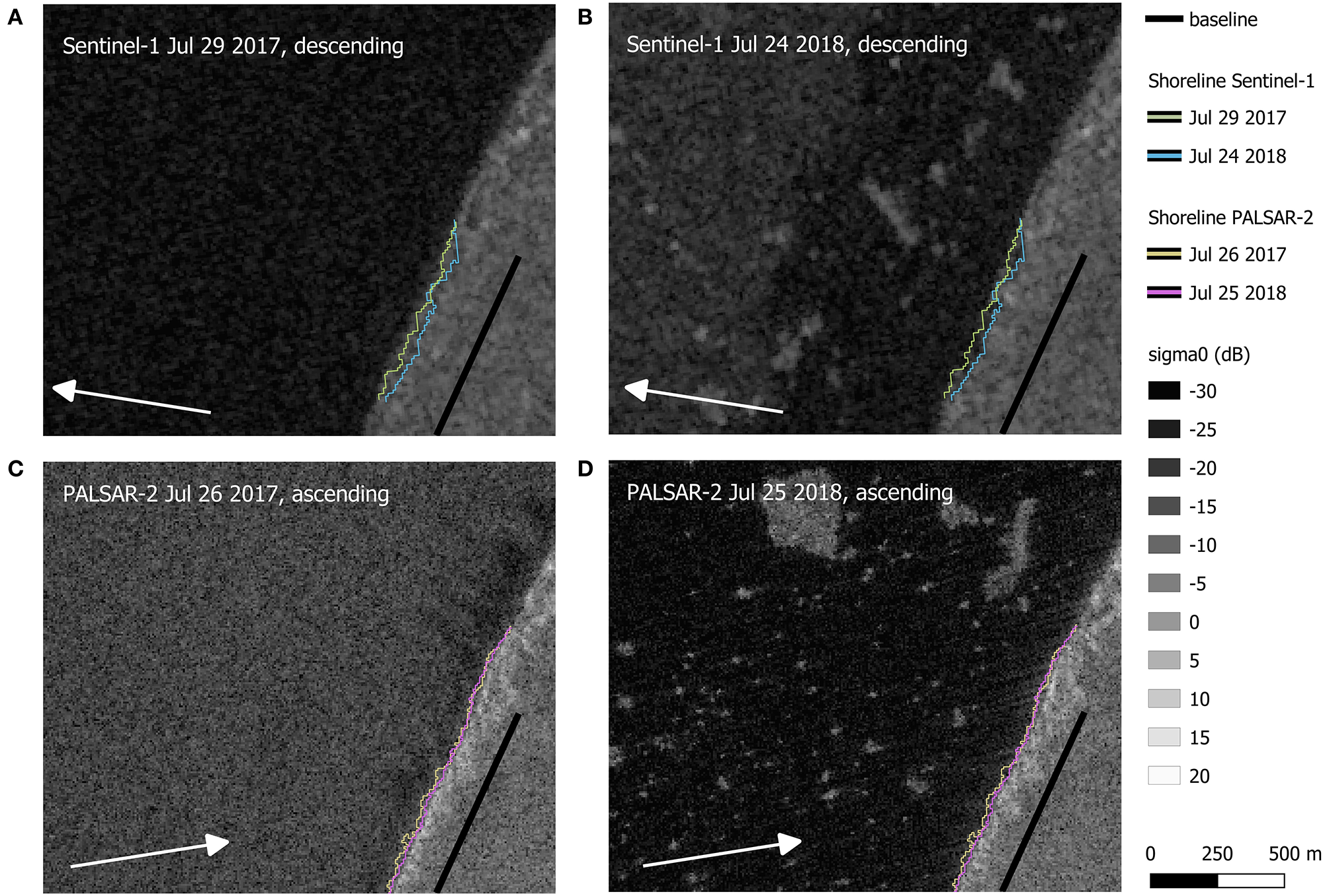
Backscatter of Sentinel-1 (top panels (A) and (B), acquired on descending orbit, VV polarization) and PALSAR-2 (bottom panels, (C) and (D), acquired on ascending orbit, HH polarization) acquisitions at Avadlek (Herschel Island) for 2017 and 2018. Dates represent closest acquisitions between the two sensors for each year. Images are ellipsoid corrected only. Sensor viewing direction is indicated by arrows. Derived shorelines represent the land-water boundary. The baseline for retreat rate calculations corresponds to Figure 2A.
Misclassifications can be also caused by infrastructure. Buildings show high backscatter values due to foreshortening and the double-bounce effect. Smooth streets scatter almost no signal back toward the sensor (Balz and Liao, 2010). This causes misclassifications of buildings and metallic objects as steep coast and misclassifications of streets as water. The Beaufort Sea Coast and Bykovsky study areas are, however, not affected as they do not include settlements. In the Varandai region, the infrastructure misclassifications did not affect the erosion analysis because the coast is not a steep cliff. There, the land–water border was used as the coastline for the erosion analysis. This issue needs to be considered for applications over larger regions.
Wide, smooth sand beaches are in general difficult to classify, especially for longer wavelengths. The roughness of the material in comparison to the wavelength is the main factor whether a specular reflection or a scattering of the wave takes place (Jones and Vaughan, 2010). Like calm water, sand is a relatively smooth surface in comparison to the C- and L-band wavelengths, and the microwave signal is reflected in a single beam that is not directed toward the sensor. Furthermore, the radar backscatter depends on the geometric and dielectric properties of the surface. Sand has in general a very low dielectric constant, so the microwaves penetrate deep into the material. This effect further reduces the backscatter signal (Stephen and Long, 2005). This makes SAR classification of sandy areas, like parts of the Barents Sea coast, challenging. The temporal stability of the low surface roughness of these areas may, however, be of benefit for separation of sandy areas from water affected by wave action (rough surface).
Banks et al. (2014) found that for C-band the best separability of sandy areas from water was given with images in HH polarization with shallow (45.3°–49.5°) and medium (39.3°) incidence angles. However, images with steep (20.9°–24.2°) incidence angles tend to bring better separability results in VV and HV polarizations. This incidence angle range is however not available from Sentinel-1.
Wet snow can impact the classification result as shown in Figure 9 for TerraSAR-X near King Point. Snow has been still present at the June acquisition date in 2018. A comparison with the Sentinel-2 optical images demonstrates that some pixels, which were classified as water, correspond to the location of late lying snow patches. The mean temperature around 2018-06-15 in that area hovered slightly above 0°C (Government Canada, 2019), indicating that the snow was melting. Like open water, wet snow is characterized by low backscatter. Wet snow typically absorbs the microwave signal and reduces the backscatter intensity significantly (further TerraSAR-X examples in similar settings: Antonova et al., 2016; Mora et al., 2017; Stettner et al., 2018), which caused the false classification result.
Figure 9
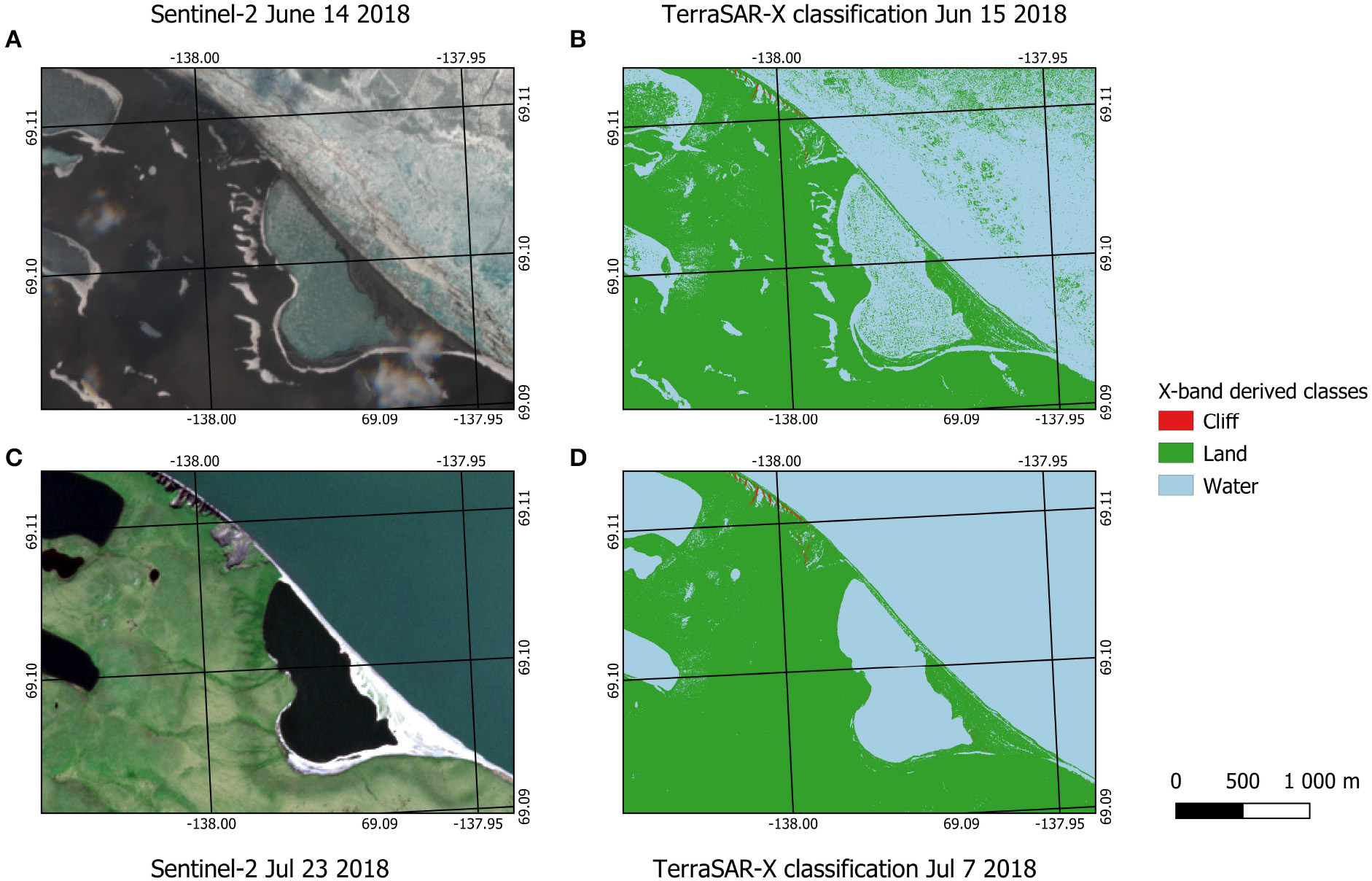
The influence of snow and ice on the classification result of TerraSAR-X at King Point (20 km south of Kay Point). Left (A) and (C): RGB (band 4, 3, and 2) composites of Sentinel-2; right (B) and (D): TerraSAR-X derived classes. Snow on land is classified as water (wet snow - low backscatter) and sea ice is partially classified as land (higher backscatter than open water). Sentinel-2 acquisitions represent closest available to TerraSAR-X acquisition.
Results indicate that also radar shadow areas can be used to quantify erosion rates in case that the spatial resolution allows clear separation. This enables identification of the cliff tops in case of bluffs facing away from the sensor in summer as well as winter. Retrievals for X-band indicate that identification of cliff-tops facing the sensor (separation from land) might be more reliable with acquisitions from the unfrozen and snow-free period as not only the foreshortening effect plays a role for the higher backscatter. Exposed wet soils contribute as well, leading to a drop in backscatter in winter (see Figure 5). The winter- summer difference at Kay Point is larger than reported in Stettner et al. (2017).
The limitation of the analysis to the ellipsoid correction allows to account for the lack of accurate digital elevation model time series. Direct comparisons between results from different viewing geometries, however, can not be made. Only the quantification of relative change is feasible, which impacts combinations with other data sources and an exact assignment to coastlines. A characterization of coastal segments (as in Lantuit et al., 2012) should be nevertheless feasible.
The high uncertainty values of the PALSAR-2 and Sentinel-1 results might be caused by the spatial resolution, which also affects which erosion processes can be monitored. Choosing a transect distance much lower than the spatial resolution will not improve the calculation results. Therefore, only erosion features larger or equal to the spatial resolution of the image can be captured. The differences in derived rates between the sensors may be also explained by the fact that the calculations assess slightly different areas due to their comparably coarse spatial resolution (mixed pixel effects) and differences in classification accuracy. The different acquisition timing also adds to that.
It would be interesting to compare change rates based on 2007–2018 C-band data with the calculated rates based on 2007–2018 PALSAR/PALSAR-2 L-band data. Unfortunately, only coarse resolution (30 m) data for the areas of interest are available for ENVISAT and ERS-1/2 (the predecessor satellites of Sentinel-1) (ESA, 2019a). Both of these SAR missions acquired data in VV polarization, which we could show to be suitable for the identification of the land-water boundary. Such data could be therefore used to derive long-term trends similar to Landsat, going back as far as 1991. Coverage across the Arctic is, however, limited due to the acquisition strategies of these missions. Future studies could include data from the operationally focused Canadian RADARSAT-2 satellite. Images with a higher resolution than 30 m were acquired for some study areas (e.g., Herschel Island) between 2008–2019 (MDA, 2019).
4.2. Erosion Rates
The only available study to date using SAR data for Arctic erosion rates was carried out for a river bank with TerraSAR-X. Stettner et al. (2017) calculated 22-day cliff-top movements based on a threshold classification for an ice-rich riverbank situated in the Lena Delta. The statistically determined threshold (cliff vs. land) for this study (approximately −2.5 dB for 31°) is higher than in Stettner et al. (2017) which determined −7.8 dB for HH (31°) based on visual evaluation. This difference may relate to mode characteristics (staring spot light in this study vs. stripmap mode in Stettner et al., 2017), strength of the foreshortening effect, and surface wetness apart from the consideration of surface type specific noise. The −7.8 dB threshold is still well above the land (tundra) average (~ −11 dB), but within one standard deviation.
Results for the Beaufort Sea Coast (Kay Point) are similar to results published by Irrgang et al. (2018) (Table 5). They calculated shoreline movements of the Yukon Coast based on aerial and satellite images between the years 1951 and 2011. Average rates for the entire coast segment are in the order of the maximum in case of all sensors, specifically PALSAR-1/2 and Landsat which provide long-term rates with lower uncertainties than the annual retrievals. The differences suggest higher rates in recent years for this site, but the uncertainties (±−0.4 m and ±−1.4 m, respectively) are still high compared to the observed range in Irrgang et al. (2018, −0.8 to −4.1 m).
Obu et al. (2016) used aerial lidar elevation data from 2012 and 2013 with a horizontal resolution of 1 m to study short-term coastal erosion at the Yukon Coast including Herschel Island. Rates are reported for the land-water boundary. The results are also consistent with this study. Their calculated coastline movement for this area is −6.8 m/year (Obu et al., 2016), which is similar to the long-term results (2007–2018) of this study (−7.02 m/year). Landsat estimates are, however, lower with −4.19 m/year for the period 1999–2014. Mean annual ground temperature has been increasing by 3°C from 2003 to 2017 (Figure 10). This may suggest higher rates in recent years, but differences in spatial resolution may reduce the comparability of results. Larger fluctuations from year to year within the different analyses periods could also contribute to this difference.
Figure 10
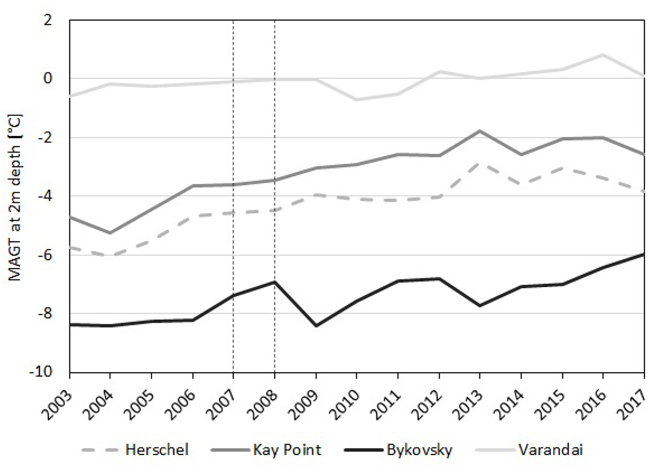
Mean annual ground temperature (MAGT) at 2 m depth for 2003–2017 (source: Obu et al., 2019a). Vertical dashed lines indicate years with PALSAR acquisitions.
Coastal erosion dynamics on Bykovsky Peninsula were calculated between 1951 and 2006 by Lantuit et al. (2011). They analyzed airborne and spaceborne optical images and calculated the annual erosion rates. Rates of up to 2 m/year (Lantuit et al., 2011) were determined at the coastal stretch selected in our study. The agreement among the sensors for the recent development (up to about 10 m/year) suggests an increase of erosion activity at this site as well, but uncertainties are also very high (Table 5). However, this agrees with findings by Günther et al. (2015) at the nearby Muostakh island for 2010–2013. The time series of mean annual ground temperature indicates an increase of 2°C in this region between 2003 and 2017 (Figure 10).
While cliff-top retreat (thermo-denudation) was faster than the land-water boundary change (thermo-abrasion) at Muostakh (10.2 m vs. 3.4 m/year), it appears rather similar at the Bykovsky site (Table 5). The analyzed Muostakh sections face mostly North-East, whereas the Bykovsky site exposition is West. As thermo-abrasion conditions thermo-denudation (Günther et al., 2015), the differences among the sites (also compared to Herschel where the land-water boundary change exceeds cliff top retreat) may represent different stages of interaction. The analyses of longer time series with annual resolution might provide more insight into the related mechanisms and dependencies.
Leont'yev (2003) predicted that the open coast of Varandai would retreat 300 to 500 m over the next century, or 3 to 5 m/year. This study's calculated 2007–2018 erosion rate of 5.41 m/year is slightly faster than Leont'yev's rate, but matches within the uncertainty. Surprisingly, the two year-to-year rates calculated in this study were very close to Leont'yev's rate, even though their uncertainties are still extremely large. As mentioned before, it is challenging to distinguish between tidal and wave motion and erosion processes in sand areas without vegetation or cliffs. The tidal motion can cause calculation errors as the position of the land-water boundary is affected. Rates for 1951–2013 as reported by Sinitsyn et al. (2020) are lower with 1.8 m/years. Rates seem to have increased at Varandai as well. The rates in 2007/8 and 2017/18 are similar (about 3m) as was also mean annual ground temperature (Figure 10).
5. Conclusions
In general, the calculation of long-term shoreline movements of sensor facing steep coasts in the Arctic based on a threshold classification seems to be a promising approach. The calculated rates based on PALSAR/PALSAR-2 L-band images between 2007 and 2018 seem to bring reasonable results. The uncertainties are, however, high for the prediction of short-term trends based on Sentinel-1 and PALSAR-2 images, which have comparably low-resolution (10 and 12.5 m nominal resolution, respectively) with respect to actual erosion rates. This may be improved by using more than one image per year. Another limitation of such resolution is that only erosion features equal to or greater than the resolution of the image can be detected.
In addition to Stettner et al. (2017), who focused on cliffs facing the sensor, we demonstrated the utility of SAR data for separation of the land-water boundary at Arctic coasts. This expands the potential of SAR application, as sensor facing cliffs are only relevant in case of (1) presence of cliffs and (2) coast orientation toward the West or the East. The identification of such coastal segments can be based on using existing landcover datasets in conjunction with orbit inclination information as presented in this paper.
The comparison of the classification results with optical data revealed several issues: snow, wide sand beaches, and infrastructure. In the classification results, wet snow was misclassified as water, which made classifications during snow melt difficult. Late lying snow patches can also occur at North-facing slopes. In future work, including a threshold function to determine snow melt may help avoid possible misclassifications.
Classification is also complicated by smooth sand beaches. The sand backscatter values of long-wave C-band and L-band microwaves are relatively low, which makes the distinction between water and sand challenging. Future studies may overcome this by introducing an additional class for land, by distinguishing between sandy areas and undisturbed tundra.
A comparison of the PALSAR/PALSAR-2 L-band long-term results of this study with RADARSAT-2 C-band long-term results would be an interesting approach for future studies. Also, the calculation of seasonal trends with TerraSAR-X data in a region with more active erosion would be a promising application, which should be investigated. The threshold based method can help to better understand the seasonal, annual, and inter-annual Arctic coastline dynamics, and it provides additional information that complements the optical and in situ methods. In a further step machine-learning methods can be introduced to analyze coastlines with a higher degree of automation and reliability.
The consideration of incidence angles to distinguish relevant surface types is required for cliff-land as well as land-water discrimination in case of L-band. In case of C-band it is only required for land-water discrimination. The variation of backscatter in X-band data is specifically high for water. But our results suggest that incidence angle dependencies are not required to be considered for this type of application of X-band data at HH polarization. High incidence angles might be of benefit due to the impact of incidence angle on spatial resolution in staring spot light mode.
Specifically L-band data could be shown of benefit due to their lower sensitivity to wave action. C-band, specifically Sentinel-1, can be, however, also utilized and provides similar estimates like other sensors in case of calm sea. Several future L-band SAR missions are currently in planning [NISAR, ROSE-L NASA (2019); Pierdicca et al. (2019)] which could be of interest for coastal erosion studies over larger areas in the future. The post processed Landsat derived trends provide an additional source for longterm monitoring, specifically for automatic retrieval across the entire Arctic. This could be complemented by ENVISAT and ERS-1/2 C-band SAR data for the period 1991 to 2012. Superior regarding spatial resolution and at the same time also illumination independence is TerraSAR-X. The nominal resolution of 1 m or better may not only allow determination of sub-seasonal retreat rates at some of the sites, but also the separation of radar shadow at high bluffs enables the identification of the cliff-top position.
Statements
Data availability statement
The raw data supporting the conclusions of this article will be made available by the authors, without undue reservation.
Author contributions
AB contributed conception and design of the study. SL organized the database. SL, AB, and GP performed the SAR data and statistical analysis. IN performed the Landsat data trend analysis, AB the post-processing. AB and SL wrote the first draft of the manuscript. GV supported procurement and selection of TerraSAR-X sites and acquisitions. All authors contributed to manuscript revision, read and approved the submitted version.
Funding
The authors acknowledge financial support by the HORIZON2020 (BG-2017-1) project Nunataryuk, ESA's DUE GlobPermafrost project (Contract Number 4000116196/15/I-NB), ESA's CCI+ Permafrost (4000123681/18/I-NB), the FFG FemTech projects CoastSAR (874213) and CoastAIMap (880182).
Acknowledgments
We acknowledge the coordination of TerraSAR-X acquisitions through the WMO Polar Space Task Group, specifically Achim Roth. All TerraSAR-X data were made available by the German Aerospace Center (DLR) through PI agreement COA3645. All ALOS PALSAR and PALSAR-2 data were made available by the Japanese Space Agency (JAXA) through PI agreement 3068002. Results are partially based on modified Copernicus data from 2017 to 2018. We further thank Aleksandra Efimova (b.geos) for supporting part of the GIS tasks.
Conflict of interest
The authors declare that the research was conducted in the absence of any commercial or financial relationships that could be construed as a potential conflict of interest.
References
1
AntonovaS.DuguayC.KaabA.HeimB.LangerM.WestermannS.BoikeJ. (2016). Monitoring bedfast ice and ice phenology in lakes of the Lena River delta using TerraSAR-X backscatter and coherent time series. Remote Sens. 8:903. 10.3390/rs8110903
2
ArpC. D.JonesB. M.SchmutzJ. A.UrbanF. E.JorgensonM. T. (2010). Two mechanisms of aquatic and terrestial habitat change along an Alaskan Arctic coastline. Polar Biol. 33, 1629–1640. 10.1007/s00300-010-0800-5
3
ASF (2019). MapReady. Version 3.1.24. Available online at: https://www.asf.alaska.edu/data-tools/mapready
4
BalzT.LiaoM. (2010). Building-damage detection using post-seismic high-resolution SAR satellite data. Int. J. Remote Sens. 31, 3369–3391. 10.1080/01431161003727671
5
BanksS. N.KingD. J.MerzoukiA.DuffJ. (2014). Assessing RADARSAT-2 for mapping shoreline cleanup and assessment technique (SCAT) classes in the Canadian Arctic. Can. J. Remote Sens. 40, 243–267. 10.1080/07038992.2014.968276
6
BartschA.HöflerA.KroisleitnerC.TrofaierA. M. (2016). Land cover mapping in northern high latitude permafrost regions with satellite data: achievements and remaining challenges. Remote Sens. 8:979. 10.3390/rs8120979
7
BartschA.LeibmanM.StrozziT.KhomutovA.WidhalmB.BabkinaE.et al. (2019a). Seasonal progression of ground displacement identified with satellite radar interferometry and the impact of unusually warm conditions on permafrost at the Yamal Peninsula in 2016. Remote Sens. 11:1865. 10.3390/rs11161865
8
BartschA.PointnerG.LeibmanM. O.DvornikovY. A.KhomutovA. V.TrofaierA. M. (2017). Circumpolar mapping of ground-fast lake ice. Front. Earth Sci. 5:12. 10.3389/feart.2017.00012
9
BartschA.WidhalmB.LeibmanM.ErmokhinaK.KumpulaT.SkarinA.et al. (2020). Feasibility of tundra vegetation height retrieval from Sentinel-1 and Sentinel-2 data. Remote Sens. Environ. 237:111515. 10.1016/j.rse.2019.111515
10
BartschA.WidhalmB.PointnerG.ErmokhinaK.LeibmanM.HeimB. (2019b). Landcover Derived From Sentinel-1 and Sentinel-2 Satellite Data (2015-2018) for Subarctic and Arctic Environments. PANGAEA. 10.1594/PANGAEA.897916
11
CoutureN. J.IrrgangA.PollardW.LantuitH.FritzM. (2018). Coastal erosion of permafrost soils along the yukon coastal plain and fluxes of organic carbon to the Canadian Beaufort Sea. J. Geophys. Res. Biogeosci. 123, 406–422. 10.1002/2017JG004166
12
CunliffeA. C.TanksiG.RadosavljevicB.PalmerW. F.SachsT.LanuitH.et al. (2019). Rapid retreat of permafrost coastline observed with aerial drone photogrammetry. Cryosphere13, 1513–1528. 10.5194/tc-13-1513-2019
13
DouglasD. H.PeuckerT. K. (1973). Algorithms for the reduction of the number of points required to represent a digitized line or its caricature. Cartographica10, 112–122. 10.3138/FM57-6770-U75U-7727
14
ESA (2012). Sentinel-1. ESA's Radar Observatory Mission for GMES Operational Services. Technical report.
15
ESA (2015). Sentinel-2 User Handbook. Technical report.
16
ESA (2019a). ESA Online Catalogue. Available online at: http://esar-ds.eo.esa.int/socat/ASA_IMP_1P (accessed September 1, 2019).
17
ESA (2019b). Sentinel Application Platform (SNAP). Available online at: http://step.esa.int/main/toolboxes/snap
18
ForbesD. L.SolomonS. M.FrobelD. (1995). Report of 1992 Coastal Surveys in the Beaufort Sea. Technical report. 10.4095/203482
19
FrederickJ. M.ThomasM. A.BullD. L.JonesC. A.RobertsJ. D. (2016). The Arctic Coastal Erosion Problem. Technical report, Sandia National Laboratories. 10.2172/1431492
20
Government Canada (2019). Historical Climate Data. Available online at: http://climate.weather.gc.ca/historical_data/search_historic_data_e.html (accessed July 15, 2019).
21
GrosseG.SchirrmeisterL.KunitskyV. W.HubbertenH.-W. (2005). The use of CORONA images in remote sensing of periglacial geomorphology: an illustration from the NE Sibirian Coast. Permafrost Periglacial Process. 16, 163–172. 10.1002/ppp.509
22
GuéganE. B. M.ChristiansenH. H. (2016). Seasonal arctic coastal bluff dynamics in Adventfjorden, Svalbard. Permafrost Periglacial Process. 28, 18–31. 10.1002/ppp.1891
23
GüntherF.OverduinP. P.SandakovA. V.GrosseG.GrigorievM. N. (2013). Short- and long-term thermo-erosion of ice-rich permafrost coasts in the Laptev Sea region. Biogeosciences10, 4297–4318. 10.5194/bg-10-4297-2013
24
GüntherF.OverduinP. P.YakshinaL. A.OpelT.BaranskayaA. V.GrigorievM. N. (2015). Observing Muostakh disappear: permafrost thaw subsidence and erosion of a ground-ice-rich island in response to arctic summer warming and sea ice reduction. Cryosphere9, 151–178. 10.5194/tc-9-151-2015
25
HequetteA.RuzM.-H.HillP. R. (1995). The effects of the Holocene sea-level rise on the evolution of the southeastern coast of the Canadian Beaufort Sea. J. Coast. Res. 11, 494–507.
26
HimmelstossE. A.HendersonR. E.KratzmannM. G.FarrisA. S. (2018). Digital Shoreline Analysis System (DSAS). ersion 5.0 User Guide. USGS.10.3133/ofr20181179
27
HoqueM. A.PollardW. H. (2004). “Modeling block failures of vertical cliffs in the Arctic Coast. Arctic Coastal Dynamic,” in Report of the 5th International Workshop (Montreal, QC: McGill University), 60–64.
28
HoqueM. A.PollardW. H. (2009). Arctic coastal retreat through block failure. Can. Geotech. J. 46, 1103–1115. 10.1139/T09-058
29
IrrgangA. M.LantuitH.GordonR. R.PiskorA.MansonG. K. (2019). Impacts of past and future coastal changes on the Yukon coast-threats for cultural sites, infrastructure, and travel routes. Arctic Sci. 5, 107–126. 10.1139/as-2017-0041
30
IrrgangA. M.LantuitH.MansonG. K.GüntherF.GrosseG.OverduinP. P. (2017). Quantification of shoreline movements along the Yukon territory mainland coast between 1951 and 2011, supplement to: Irrgang, anna maria; lantuit, hugues; manson, gavin k; guenther, frank; grosse, guido; overduin, pier paul (2018): Variability in rates of coastal change along the yukon coast, 1951 to 2015. J. Geophys. Res. Earth Surface123, 779–800. 10.1594/PANGAEA.874343
31
IrrgangA. M.LantuitH.MansonG. K.GüntherF.GrosseG.OverduinP. P. (2018). Variability in Rates of Coastal Change Along the Yukon coast, 1951 to 2015. J. Geophys. Res. Earth Surface123, 779–800. 10.1002/2017JF004326
32
JAXA (2008). ALOS Data Users Handbook. Revision C. Tokyo.
33
JAXA (2018). ALOS-2 Solution Book. Proposals for 'DAICHI 2' SAR Data Utilization, 3rd Edn. Tokyo.
34
JonesB.HinkelK. M.ArpC. D.EisnerW. R. (2008). Modern erosion rates and loss of coastal features and sites, Beaufort Sea Coastline, Alaska. Arctic61, 361–372. 10.14430/arctic44
35
JonesG. H.VaughanR. A. (2010). Remote Sensing of Vegetation. Principles, Techniques and Applications. New York, NY: Oxford University Press.
36
KroonA. (2014). “Chapter 14: High-Latitude Coasts,” in Coastal Environments and Global Change, eds G. Masselink and R. Gehrels (Chichester: John Wily & Sons), 338–353. 10.1002/9781119117261.ch14
37
LantuitH. (2008). The modification of arctic permafrost coastlines (Ph.D. thesis). Universität Potsdam, Potsdam, Germany.
38
LantuitH.AtkinsonD.OverduinP. P.GrigoriewM.RacholdV.GrosseG.HubbertenH.-W. (2011). Coastal erosion dynamics on the permafrost-dominated Bykovsky Peninsula, north Siberia, 1951-2006. Polar Res. 30:7341. 10.3402/polar.v30i0.7341
39
LantuitH.OverduinP. P.CoutureN.WetterichS.AréF.AtkinsonD.et al. (2012). The Arctic Coastal Dynamics Database: A New Classification Scheme and Statistics on Arctic Permafrost Coastlines. Estuar. Coasts35, 383–400. 10.1007/s12237-010-9362-6
40
LeT. M. H.DepinaI.GueganE.SinitsynA. (2018). Thermal regime of permafrost at Varandey Settlement along the Barents Sea Coast, North West Arctic Russia. Eng. Geol. 246, 69–81. 10.1016/j.enggeo.2018.09.026
41
LeeJ.-S.WenJ.-W.AinsworthT. L.ChenK.-S.ChenA. (2009). Improved sigma filter for speckle filtering of SAR imagery. IEEE Trans. Geosci. Remote Sens. 47, 202–213. 10.1109/TGRS.2008.2002881
42
Leont'yevI. O. (2003). Modeling erosion of sedimentary coasts in the western Russian Arctic. Coast. Eng. 47, 413–429. 10.1016/S0378-3839(02)00145-X
43
LiuL.SchaeferK.ZhangT.WahrJ. (2012). Estimating 1992-2000 average active layer thickness on the Alaskan north slope from remotely sensed surface subsidence. J. Geophys. Res. Earth Surface117:F01005. 10.1029/2011JF002041
44
MDA (2019). MDA's RADARSAT-2 Portal. Available online at: https://mdacorporation.com/geospatial/international/radarsat-portal (accessed September 1, 2019).
45
MentaschiL.VousdoukasM. I.PekelJ.-F.VoukouvalasE.FeyenL. (2018). Global long-term observations of coastal erosion and accretion. Sci. Rep. 8:12876. 10.1038/s41598-018-30904-w
46
MoraC.JiménezJ. J.PinaP.CatalãoJ.VieiraG. (2017). Evaluation of single-band snow-patch mapping using high-resolution microwave remote sensing: an application in the maritime Antarctic. Cryosphere11, 139–155. 10.5194/tc-11-139-2017
47
NASA (2019). NASA-ISRO SAR (NISAR) Mission Science Users' Handbook. CL# 18-1893, JPL 400-1707 08/19. California, CA: Jet Propulsion Laboratory; California Institute of Technology Pasadena.
48
NielsenD. M.DobryninM.BaehrJ.RazumovS.GrigorievM. (2020). Coastal erosion variability at the southern Laptev Sea linked to winter sea ice and the Arctic oscillation. Geophys. Res. Lett. 47:e2019GL086876. 10.1029/2019GL086876
49
NitzeI. (2018). Trends of Land Surface Change Fromlandsat Time-Series 1999-2014. PANGAEA - Data Publisher for Earth & Environmental Science. 10.1594/PANGAEA.884137
50
NitzeI.GrosseG.JonesB.ArpC.UlrichM.FedorovA.et al. (2017). Landsat-based trend analysis of lake dynamics across northern permafrost regions. Remote Sens. 9:640. 10.3390/rs9070640
51
NitzeI.GrosseG.JonesB. M.RomanovskyV. E.BoikeJ. (2018). Remote sensing quantifies widespread abundance of permafrost region disturbances across the Arctic and Subarctic. Nat. Commun. 9:5423. 10.1038/s41467-018-07663-3
52
ObuJ.LantuitH.GrosseG.GüntherF.SachsT.HelmV.et al. (2016). Coast erosion and mass wasting along the Canadian Beaufort Seas based on annual airborne LiDAR elevation data. Geomorphology293, 331–346. 10.1016/j.geomorph.2016.02.014
53
ObuJ.WestermannS.BarbouxC.BartschA.DelaloyeR.GrosseG.et al. (2019a). ESA Permafrost Climate Change Initiative (Permafrost_cci): Permafrost Ground Temperature for the Northern Hemisphere, Centre for Environmental Data Analysis (CEDA). 10.5285/9A333481E9A34C7A8F78902F77AD3FE7
54
ObuJ.WestermannS.BartschA.BerdnikovN.ChristiansenH. H.DashtserenA.et al. (2019b). Northern hemisphere permafrost map based on TTOP modelling for 2000-2016 at 1 km2 scale. Earth Sci. Rev. 193, 299–316. 10.1016/j.earscirev.2019.04.023
55
OverlandJ.DunleaE.BoxJ. E.CorellR.ForsiusM.KattsovV.et al. (2019). The urgency of Arctic change. Polar Sci. 21, 6–13. 10.1016/j.polar.2018.11.008
56
PierdiccaN.DavidsonM.ChiniM.DierkingW.DjavidniaS.HaarpaintnerJ.et al. (2019). “The Copernicus L-band SAR mission ROSE-L (Radar Observing System for Europe) (Conference Presentation),” in Proc. SPIE 11154, Active and Passive Microwave Remote Sensing for Environmental Monitoring III. 10.1117/12.2534743
57
RadosavljevicB.LantuitH.PollardW.OverduinP.CoutureN.SachsT.et al. (2016). Erosion and flooding–threats to coastal infrastructure in the Arctic: a case study from Herschel Island, Yukon Territory, Canada. Estuar. Coasts39, 900–915. 10.1007/s12237-015-0046-0
58
RomeiserR.HorstmannJ.CarusoM. J.GraberH. C. (2013). A descalloping postprocessor for ScanSAR images of ocean scenes. IEEE Trans. Geosci. Remote Sens. 51, 3259–3272. 10.1109/TGRS.2012.2222648
59
SchubertA.MirandaN.GeudtnerD.SmallD. (2017). Sentinel-1A/B combined product geolocation accuracy. Remote Sens. 9:607. 10.3390/rs9060607
60
SchusterP. F.SchaeferK. M.AikenG. R.AntweilerR. C.DewildJ. F.GryziecJ. D.et al. (2018). Permafrost stores a globally significant amount of mercury. Geophys. Res. Lett. 45, 1463–1471. 10.1002/2017GL075571
61
ShimadaM. (2009). “Advance land-observation satellite (ALOS) and its follow-on satellite, ALOS-2,” in Proceedings of the 4th International POLinSAR 2009 Workshop, ESA/ESRIN (Frascati).
62
ShortN.BriscoB.CoutureN.PollardW.MurnaghanK.BudkewitschP. (2011). A comparison of TerraSAR-X, RASARSAT-2 and ALOS-PALSAR interferometry for monitoring permafrost environments, case study from Herschel Island, Canada. Remote Sens. Environ. 115, 3491–3506. 10.1016/j.rse.2011.08.012
63
SinitsynA. O.GueganE.ShabanovaN.KokinO.OgorodovS. (2020). Fifty four years of coastal erosion and hydrometeorological parameters in the Varandey region, Barents Sea. Coast. Eng. 157:103610. 10.1016/j.coastaleng.2019.103610
64
SolomonS. M. (2005). Spatial and temporal variability of shoreline change in the Beaufort-Mackenzie region, northwest territories, Canada. Geomar. Lett. 25, 127–137. 10.1007/s00367-004-0194-x
65
SteeleM.ErmoldW.ZhangJ. (2008). Arctic Ocean surface warming trends over the past 100 years. Geophys. Res. Lett. 35:L02614. 10.1029/2007GL031651
66
StephenH.LongD. G. (2005). Microwave backscatter modeling of erg surfaces in the Sahara Desert. IEEE Trans. Geosci. Remote Sens. 43, 238–247. 10.1109/TGRS.2004.840646
67
StettnerS.BeamishA.BartschA.HeimB.GrosseG.RothA.et al. (2017). Monitoring inter- and intra-seasonal dynamics of rapidly degrading ice-rich permafrost riverbanks in the Lena Delta with TerraSAR-x time series. Remote Sens. 10:51. 10.3390/rs10010051
68
StettnerS.LantuitH.HeimB.EpplerJ.RothA.BartschA.et al. (2018). TerraSAR-X time series fill a gap in spaceborne snowmelt monitoring of small arctic catchments–a case study on Qikiqtaruk (Herschel Island), Canada. Remote Sens. 10:1155. 10.3390/rs10071155
69
StrozziT.AntonovaS.GüntherF.MätzlerE.VieiraG.WegmüllerU.et al. (2018). Sentinel-1 SAR interferometry for surface deformation monitoring in low-land permafrost areas. Remote Sens. 10:1360. 10.3390/rs10091360
70
WidhalmB.BartschA.GolerR. (2018). Simplified normalization of C-band synthetic aperture radar data for terrestrial applications in high latitude environments. Remote Sens. 10:551. 10.3390/rs10040551
71
ZwiebackS.KokeljS. V.GüntherF.BoikeJ.GrosseG.HajnsekI. (2018). Sub-seasonal thaw slump mass wasting is not consistently energy limited at the landscape scale. Cryosphere12, 549–564. 10.5194/tc-12-549-2018
Summary
Keywords
Arctic, erosion, SAR, radar, coast, permafrost
Citation
Bartsch A, Ley S, Nitze I, Pointner G and Vieira G (2020) Feasibility Study for the Application of Synthetic Aperture Radar for Coastal Erosion Rate Quantification Across the Arctic. Front. Environ. Sci. 8:143. doi: 10.3389/fenvs.2020.00143
Received
03 May 2020
Accepted
28 July 2020
Published
08 September 2020
Volume
8 - 2020
Edited by
Louise Farquharson, University of Alaska Fairbanks, United States
Reviewed by
Melanie Engram, University of Alaska Fairbanks, United States; Ann Gibbs, United States Geological Survey, United States; Philipp Bernhard, ETH Zürich, Switzerland
Updates
Copyright
© 2020 Bartsch, Ley, Nitze, Pointner and Vieira.
This is an open-access article distributed under the terms of the Creative Commons Attribution License (CC BY). The use, distribution or reproduction in other forums is permitted, provided the original author(s) and the copyright owner(s) are credited and that the original publication in this journal is cited, in accordance with accepted academic practice. No use, distribution or reproduction is permitted which does not comply with these terms.
*Correspondence: Annett Bartsch annett.bartsch@bgeos.com
This article was submitted to Environmental Informatics and Remote Sensing, a section of the journal Frontiers in Environmental Science
Disclaimer
All claims expressed in this article are solely those of the authors and do not necessarily represent those of their affiliated organizations, or those of the publisher, the editors and the reviewers. Any product that may be evaluated in this article or claim that may be made by its manufacturer is not guaranteed or endorsed by the publisher.