Development of High Resolution and Homogenized Gridded Land Surface Air Temperature Data: A Case Study Over Pan-East Asia

Introduction

Land Surface Air Temperature (LSAT) is considered one of the important indicators of the global and regional climate change. Many studies have shown that the global LSAT change can greatly impact on human being as well as the social and economic society (Köppen, 1931; Callendar, 1938, 1961; Hawkins and Jones, 2013). Major issues in studying the LSAT variations and change are associated with the inconsistency in observing times, uneven spatial distribution of LSAT stations, differences in statistical methods, and the quality of the observational data over global or continental regions at century scale. To resolve these issues, scientists developed homogenized station datasets and converted them into gridded datasets for the convenience of applications (Hutchinson, 1991; Daly et al., 1994; Li and Li, 2007; Xu et al., 2009). For global large-scale climate temperature trend estimation using low-resolution datasets (normally in 5° × 5° resolution to avoid changes at small scales) (Jones and Briffa, 1992; Peterson and Vose, 1997; Hansen et al., 1999; Li et al., 2017; Xu C. et al., 2018; Yun et al., 2019) can basically meet the accuracy requirements. For example, a consistent outcome from available low-resolution data sets is that the global land temperature trend since 1880 has become more and more significant (Li et al., 2020).

In contrast, high-resolution datasets (both the climatology and the anomaly time series) are widely and urgently needed (Huang et al., 2020; Xu et al., 2020) for research in climate change monitoring and climate model validation and development in regional/local scales. However, it is not easy to develop a high-resolution global and regional datasets due to the problems such as the uneven distribution and difference in the length of observation records. New et al. (1999a,b) used the Thin Plate Spline (TPS) method and angular weighting method to develop the first relatively high-resolution (0.5° × 0.5°) global LSAT climatology and anomaly dataset based on the CRU (Climatic Research Unit) LSAT station dataset, and the Climate Research Unit gridded Time series (CRU TS) has been produced and shared openly to facilitate research and analysis in all areas related to climate and climate change since the first version was released in 2000. CRU TS Version 4 (CRU TS4) is the first major update since version 3 was published in 2013 (Harris et al., 2020). The US Berkeley Earth Program team developed LSAT climatology and anomaly dataset at high-resolution (1.0° × 1.0°) – Berkeley Earth Surface Temperature (BEST) using Kriging and Inverse Distance Weighting (IDW) methods (Rohde et al., 2013). Besides, Hijmans et al. (2005) developed a global (excluding the Antarctic) high resolution climatology datasets of 1 km × 1 km resolution from 1950 to 2000, and they concluded that the use of the digital elevation model (DEM) is necessary when developing high-resolution grid data; and Fick and Hijmans (2017) further updated the datasets from 1970 to 2000 in some regions by using satellite observations and elevation data as covariates, and upgraded a new high-resolution datasets (also in 1 km × 1 km resolution). In addition, observational stations are relatively sparse in some regions in Asia (Tibet Mountains), South America, Africa, etc., and data before 1950 is relatively limited. The records in these regions are very precious for global climate change studies, while the sparse observations sometimes resulted in deficiencies in describing regional climate and climate change with the global high-resolution datasets (Li et al., 2007). Therefore, with the continuous improvement of data collection and data quality, it is inevitable to develop new high-quality global climate datasets.

Various high-resolution climate datasets at the regional scale have been developed in many countries in recent years. These countries include China (Hong et al., 2005; Xie et al., 2007; Yatagai et al., 2009; Wu and Gao, 2013; Peng et al., 2019; Huang et al., 2020; Xu et al., 2020), India (Sinha et al., 2006), Southeast Asia (Van den Besselaar et al., 2017), Europe (Nynke et al., 2009), the United States (Price et al., 2004), Australia (Hutchinson, 1991), etc., which provide good supports to climate change research at regional scales. However, there exist some obvious difference in accuracy due to the different station number, data quality control and homogenization processing in the basic dataset used by each developer. Moreover, the high-resolution datasets are sometimes difficult to be developed at the continental or global scales due to different processing methods or parameterization schemes. Some high-resolution datasets emphasized the improvement of the spatial distribution of stations but did not make the necessary assessments for the inhomogeneity due to the station number changes, which will have problems in long-term climate change trend detection (Li et al., 2007). Therefore, it is of vital importance to enhance the collection of the station data and the in-depth evaluation of the data accuracy in some regions with few observations, such as South America, Antarctica and Africa for the existing global dataset; and it is also important to develop new high quality, global, high-resolution climate datasets.

The ultimate goal of this study is to develop a global high-resolution gridded LSAT data set based on C-LSAT, a monthly global LSAT dataset developed by Chinese scientists recently (Xu W. et al., 2018; Li et al., 2020). However, C-LSAT is only a 5° × 5° anomaly dataset used to determine the long-term changes of large-scale land surface air temperature. It is necessary to develop a new higher resolution (0.5° × 0.5°) dataset, which can describe the spatial details of LSAT change at smaller scales. In this manuscript, we take the pan-East Asian region as the research region, which has numerous stations and complex terrains (including coasts, large plateaus, basins, plains and undulating areas), to test our high-resolution gridding model, so as to provide a basis for the subsequent high-resolution gridding for global area.

The remainder of this paper is arranged as follows: Section “Data Sources and Methods” introduces the main data sources, interpolation methods and validation methods used to develop high resolution gridded LSAT datasets in this paper. The interpolation and validation results of climatology and anomaly data are presented in Sections “Climatology Interpolation” and “Interpolation and Validation of LSAT Anomaly,” respectively. Section “Regional LSAT Warming Trends Analysis” discusses the regional warming trend with the newly interpolated LSAT anomaly data and the comparison with new CRU TS4 dataset. Section “Conclusion” provides final discussion and conclusions.

Data Sources and Methods

Data Sources

In this study, the observational station data is derived from C-LSAT, a monthly global LSAT dataset developed by Chinese scientists recently (Xu W. et al., 2018). This dataset has been systematically homogenized and updated by Yun et al. (2019) and Li et al. (2020). The advantage of this dataset is that it has used more observational stations compared to other similar global datasets, and the elements include monthly mean 2 m air temperature (Tavg), daily maximum (Tmax), and minimum (Tmin) temperature for the period from 1850 to 2019 (however, we only intercepts the data from 1901 to 2018 in this paper for analysis).

A rectangular region (10–60°N, 60–150°E, see Figure 1 below) was selected to test interpolation methods used in this paper. The region encompasses the key areas affected by both the Indian and East Asian monsoon. From the topographic perspective, the region contains high-altitude areas of the Qinghai-Tibet Plateau, low-altitude plain areas of the middle and lower reaches of the Yangtze River, undulating terrain areas of southwest China and central Asia, and ocean areas of western Pacific and Indian Ocean. There are a total of about 2800 observational stations in this region, and the distribution of the stations is very uneven with few stations in some parts and dense coverage in others. The region is referred to as “Pan-East Asia” henceforth for interpolation experiments and validation.

FIGURE 1

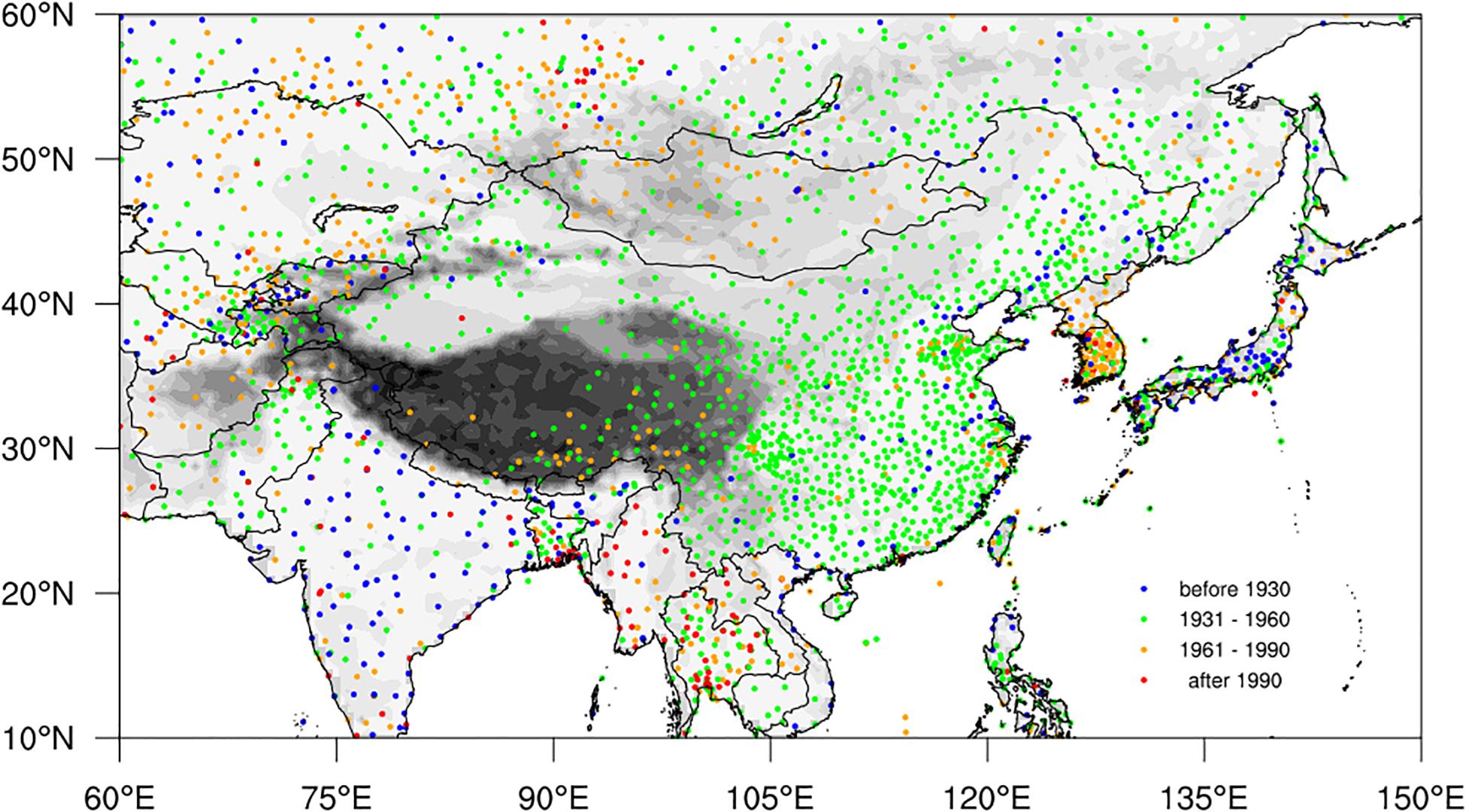
Figure 1. Spatial distribution of the observational stations in the C-LSAT2.0 dataset in the Pan-East Asia regions. The different colored dots represent stations with different starting years (SY) of observations.

Figure 1 shows the spatial distribution of the observational stations in the C-LSAT2.0 dataset in Pan-East Asia regions, and classifies the start year (SY) of the data series for each station. Many weather stations were established in India, Japan and other countries before 1930. The observation stations established in China before 1930 were mainly located in the eastern parts of the country, and most of them were built by meteorological enthusiasts or foreign missionaries (Li et al., 2020). A large number of basic and standard meteorological stations (currently about 825 stations) were set up after 1949. The Indochina peninsula has a relatively sparse density station network, and the stations with long data series are mainly located in coastal regions. Many stations have been built in Indochina peninsula and Korean peninsula after 1960, and the record length is relatively short.

Figure 2 shows the change of the station numbers in the Pan-East Asia regions during the period from 1901 to 2018 for the monthly LSAT, maximum and minimum temperature. Obviously, the station numbers of maximum and minimum temperature were less than those of average LSAT, but the overall change shape is similar.

FIGURE 2

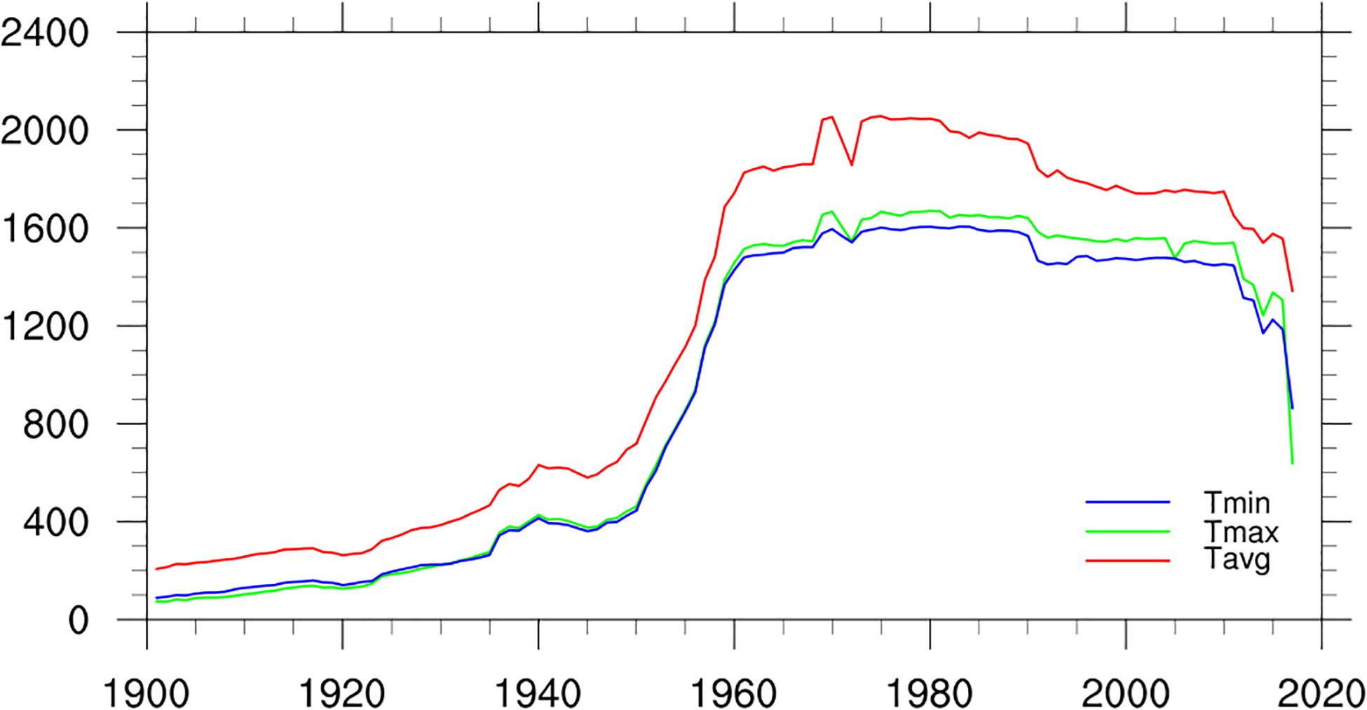
Figure 2. The number of stations in gridding region over time.

Taking the average LSAT as an example, before the 1930s, the number of stations in Pan-East Asia was less than 500. From the 1930s to the 1960s, the number of stations gradually increased, especially from less than 800 stations in the 1950s to nearly 2,000 stations in the 1960s. The number of stations with records reached the peak and remains stable during the 1960s–1990s. In this period, the number of stations with observed data is the greatest, and the number of stations that can calculate the climatology and LSAT anomaly is also the greatest. This is why we choose 1961–1990 as the base period for calculating the climatology. Further decrease of the station number in recent years may be related to the lagging of data collection and sharing.

Altitude has a significant influence on the LSAT distribution at local scales, so the digital elevation model (DEM) is usually one of the most important factors to be considered in the interpolation of LSAT, especially climatological LSAT. Previous comparison (Ma and Li, 2006) showed that although the Shuttle Radar Topography Mission (SRTM) DEM30 (which is generally recognized as having higher global average accuracy) (Farr et al., 2007) has some advantages globally, there are a little more missing areas of SRTM DEM30 based on the radar mapping of the space shuttle in complex terrain areas such as the Tibet Plateau, resulting in lower accuracy than GTOPO30 (a global 30 arc-second elevation data) in these areas; In addition, it only includes the DEM between 60°N and 60°S. So in this paper, the GTOPO30 is still used for the interpolation of the LSAT including average, maximum, and minimum LSATs similar to Xu et al. (2020).

Interpolation Schemes and Methods

In the interpolation process, the spatial density and distribution of the observational stations have great influence on the results. Studies indicated that the direct use of absolute temperature data for long term and large area interpolation are not desirable (Li et al., 2007). A common method is first to interpolate climatology and anomaly separately, and then to merge the interpolated climatology and anomaly (New et al., 1999b; Haylock et al., 2008; Rohde et al., 2013).

Based on the above procedure, the LSAT data are divided into two parts: climatology (1961–1990 average) and anomaly. A three-step procedure was adopted to grid the LSAT data: (1) the effective station data are used for interpolation of the LSAT climatology field; (2) the interpolation of LSAT anomaly field using effective station anomaly series; and (3) the final grid dataset by adding up the climatology and the anomaly gridded dataset. This gridding approach is widely used by many climate data research groups to build global and regional dataset products. For example, the CRU TS1, TS2 and the Berkeley earth surface temperature (Berkeley Earth) used a similar approach to construct the LSAT grid datasets (New et al., 1999b; Rohde et al., 2013). In this study, we calculated the 1961–1990 averages of the stations for climatology where the effective data covers temporally no less than 20 years. Then the anomalies for the whole period are computed relative to this baseline period.

Thin-Plate Spline (TPS) Interpolation for Climatology

Using the stations during the climatological period, we interpolated them onto 0.5° × 0.5° grids with the elevation information data (GTOPO30) over Pan-East Asia as the covariates. The ANUSPLIN software package version 4.4 (Hutchinson and Xu, 2013) is used to interpolate the climatology in this paper. It is an efficient and useful tool for data transparent analysis and interpolation of multivariate data using the TPS method. It completes the process by providing comprehensive statistical analysis, data diagnostics, and spatial distribution standard errors, as well as support for multiple data inputs and multiple fitting surface outputs. The TPS method used in ANUSPLIN is a reliable way to develop the spatial interpolation of climate elements, which is widely used around the world (New et al., 1999a; Hijmans et al., 2005; Haylock et al., 2008). The partial TPS method is the core algorithm of ANUSPLIN, which was originally proposed by Wahba and Wendelberger (1980). Hutchinson applied the partial TPS to the spatial interpolation of the monthly mean climate variables (Hutchinson, 1991), and its theoretical statistical model is given as follows:

$$Z_{\text{i}}=f(x_{\text{i}})+b^{\text{T}}{y}_{\text{i}}+e_{\text{i}}(i=1,\mathrm{\dots },N)(1)$$

Where Z_i is the dependent variable with N observed data values; x_i is the spline independent variable as a multi-dimensional vector, and f is the unknown smooth function for the x_i; y_i is the independent covariate as a multidimensional vector, and b is the unknown coefficients for the y_i. Each e_i is an independent, zero mean error term with variance w_iσ², where w_i is termed the relative error variance and σ² is the error variance which is constant across all data points. It can be seen from equation (1) that: when there is no covariate, the second covariate item is ignored and the model turns back to an ordinary TPS model; on the other hand, when f(x_i) is absent, the first independent item is removed and the model reduces to a simple multivariate linear regression model. In fact, the partial thin plate smoothing spline function can be understood as a generalized standard multivariate linear regression model, while its parameters are replaced by a suitable non-parameterized smooth function (Hutchinson, 1991).

The function f and the coefficient vector b are determined by minimizing

$$\sum _{i=1}^N{\left(\frac{z_{\text{i}}-f(x_{\text{i}})-b^{\text{T}}{y}_{\text{i}}}{w_{\text{i}}}\right)}^2+\mathrm{\rho }{J}_{\text{m}}(f)(2)$$

Where J_m(f) is a measure of the complexity of f, the “roughness penalty” defined in terms of an integral of m’th order partial derivatives of f, and the smoothing parameter ρ is a positive number. As ρ approaches to zero, the fitted function approaches an exact interpolation. As ρ approaches to infinity, the function f approaches a least squares polynomial, with order depending on the order m of the roughness penalty. The value of the smoothing parameter is normally determined by minimizing a measure of predictive error of the fitted surface given by the generalized cross validation (GCV; Hutchinson, 1991). The GCV is provided as a predictive error estimate of interpolation by removing each data point and summing the square of deviation between each omitted value and the corresponding interpolation value (Xu et al., 2020). The Root Square of GCV (RGCV) is used to determine the optimum parameters for ANUSPLIN.

The TPS method is very popular because of its high efficiency and its ability to generate accurate predictions with a minimum of guiding covariates (Hutchinson, 1991; New et al., 1999a; Price et al., 2004; Hijmans et al., 2005; Hong et al., 2005; Xu et al., 2009). It is observed from the comparison with other methods such as Kriging (Rohde et al., 2013) and Prism (Daly et al., 2008) that TPS is more suitable for the interpolation of the LSAT for the selected region in and hence preferred for this study.

Interpolating Method for Anomaly

In this paper, a kind of Adjusted Inverse Distance Weighted (AIDW) method was used to interpolate the anomaly data of LSAT during the period of 1900–2018. Inverse Distance Weighted (IDW) is a common and simple spatial interpolation method, based on similarity principle which describes that if two objects are nearer (farther), their properties will be similar (different). IDW sets the distance between interpolation point and sample point as the weight to achieve the weighted average. In a specific application, a higher weight is given in the LSAT interpolation when the observation station is more close to the grid point. The principle of this method is simple and easy to understand and operate. It is suitable for the case that there are many observation stations in uniform distribution.

The general formula of the IDW is:

$$T=\sum _{i=1}^n{w}_{\text{i}}{T}_{\text{i}}(3)$$

$$w_{\text{i}}=\frac{d_{\text{i}}^{-\mathrm{\alpha }}}{{\sum }_{i=1}^n{d}_{\text{i}}^{-\mathrm{\alpha }}}(4)$$

Where, T means the temperature of the grid point to be estimated; n stands for the number of observation stations participating in the interpolation for the finite region; T_i means the temperature of each station; w_i means the distance weighting of each stations; d_i means the spatial distance from each stations to the grid point to be estimated; α is a control parameter, generally assumed to be 2. Importantly, after calculation we found that the temperature anomaly field interpolated using the equations above produces “bull eyes” (Duan et al., 2014), thus we modified the formula (3) for the specific adjustment (AIDW) as follows:

$$w_{\text{i}}=\frac{{(e^{d_i/d_0})}^{-\mathrm{\alpha }}}{{\sum }_{i=1}^n{(e^{d_i/d_0})}^{-\mathrm{\alpha }}}(5)$$

The cross validation indicate that the anomaly temperature interpolation result is better when assuming α as 4 and d₀ as 1,200 km.

Validation Methods

Cross Validation (CV) is one of the most effective tool to evaluate the performance of the interpolation method. First, the in situ observations are the most precise data and are always used as the baseline data for the validation of other data types. So it is very difficult to find other different subsets of the data for validation of the gridded dataset; second, the gridded data set is derived from the in situ observations, so we cannot use the gridded data to assess the errors of the gridded data directly, thus Cross Validation (CV) is used. CV is widely used to validate the gridded observations dataset. In our manuscript, Leave One Out CV is used, which refers to taking out one station as the test station each time, and then interpolating the estimated value from the corresponding observed values of the other remaining stations. The advantage of this method is (1) nearly all the samples will be used to train the model in any round, thus the evaluation will be more reliable; (2) no random factor affects the experimental data, thus we make sure the experiment can be duplicated. Based on the results of CV, we adopted the statistical indices of Root Mean Square Error (RMSE) and Mean Absolute Error (MAE) to evaluate the interpolation errors between the estimated and observational values. The calculation formulas of RMSE and MAE are shown as follows:

$$RMSE=\sqrt{\frac{1}{\text{n}}\sum _{i=1}^n{(X_{\text{i}}-Y_{\text{i}})}^2}(6)$$

$$MAE=\frac{1}{\text{n}}\sum _{i=1}^n\left|X_{\text{i}}-Y_{\text{i}}\right|(7)$$

Where, X_i, Y_i are the estimated value and the original observational value at each station, respectively, while n is the sample number. RMSE reflects the random error between the estimated value and the actual observed value. Moreover, it estimates the degree of dispersion for the interpolation errors. MAE reflects the systematic error and estimate the average deviation between the interpolation results and the actual observed values.

Climatology Interpolation

Selection of Model Parameters

It is well known that ANUSPLIN can form different interpolation models based on various input parameters such as independent variables, covariates and spline orders. Many studies on meteorological data interpolation treat longitude and latitude as independent variables, and elevation as independent variables or covariates in the model (Hutchinson and Xu, 2013). Different interpolation model parameters may lead to different results. For example, Hong et al. (2005) used the longitude and latitude as independent variables and elevation as a covariate, while Xu et al. (2020) argued toward use of elevation as an independent variable rather than as covariate in TPS model because of its better performance.

However, since the data used in the above studies are different in terms of data volume and coverage, we first want to determine which model parameter scheme is the most preferable one according to our own data and actual situation. We use the RGCV and RMSE to determine the proper model parameter scheme. Based on the input treatment of elevation as independent variables or covariate parameters, the test groups were divided into two large groups: altitude as independent variable in group A and as covariates parameter in group B. Then according to the order of splines 2–4, both groups were subdivided again into three experiments. Therefore, a total of six experiments were taken to be tested (see Table 1). The statistical indices of RGCV and RMSE are used to analyze the errors of 6 test experiments.

TABLE 1

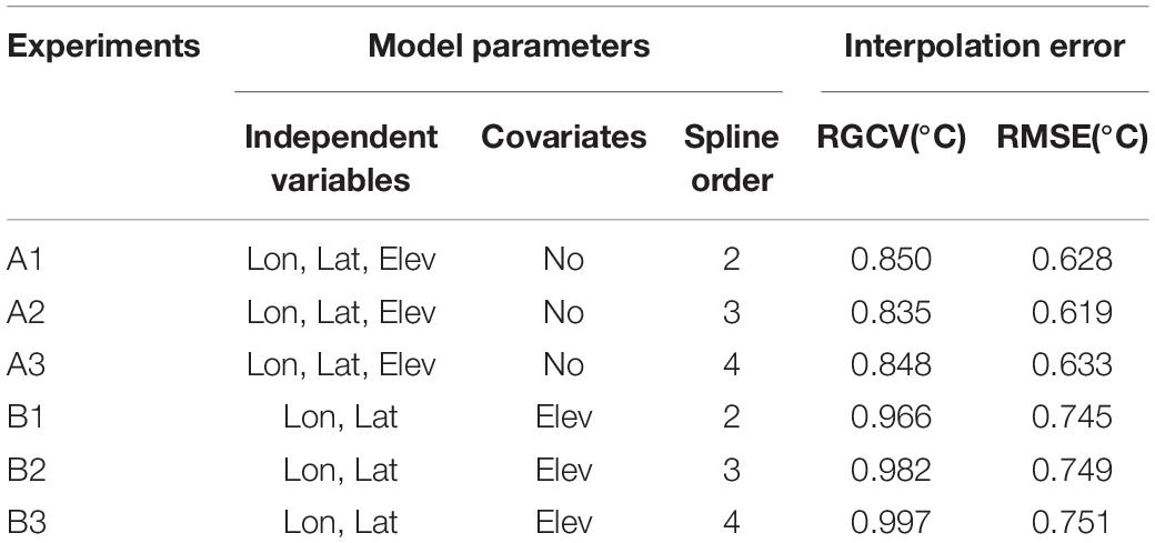
Table 1. The annual average RGCV and RMSE of the six test experiments [Ax (Bx) is the xth experiment for Group A (B)].

RGCV is one of the efficient measures of the interpolation error of the fitted surfaces provided by the ANUSPLIN software. Figure 3A shows the RGCV of the six experiments. As seen from the picture, seasonally, the RGCV in winter (December to February) is much higher than that in other seasons, and the RGCVs of group B are higher than those of group A, especially in winter.

FIGURE 3

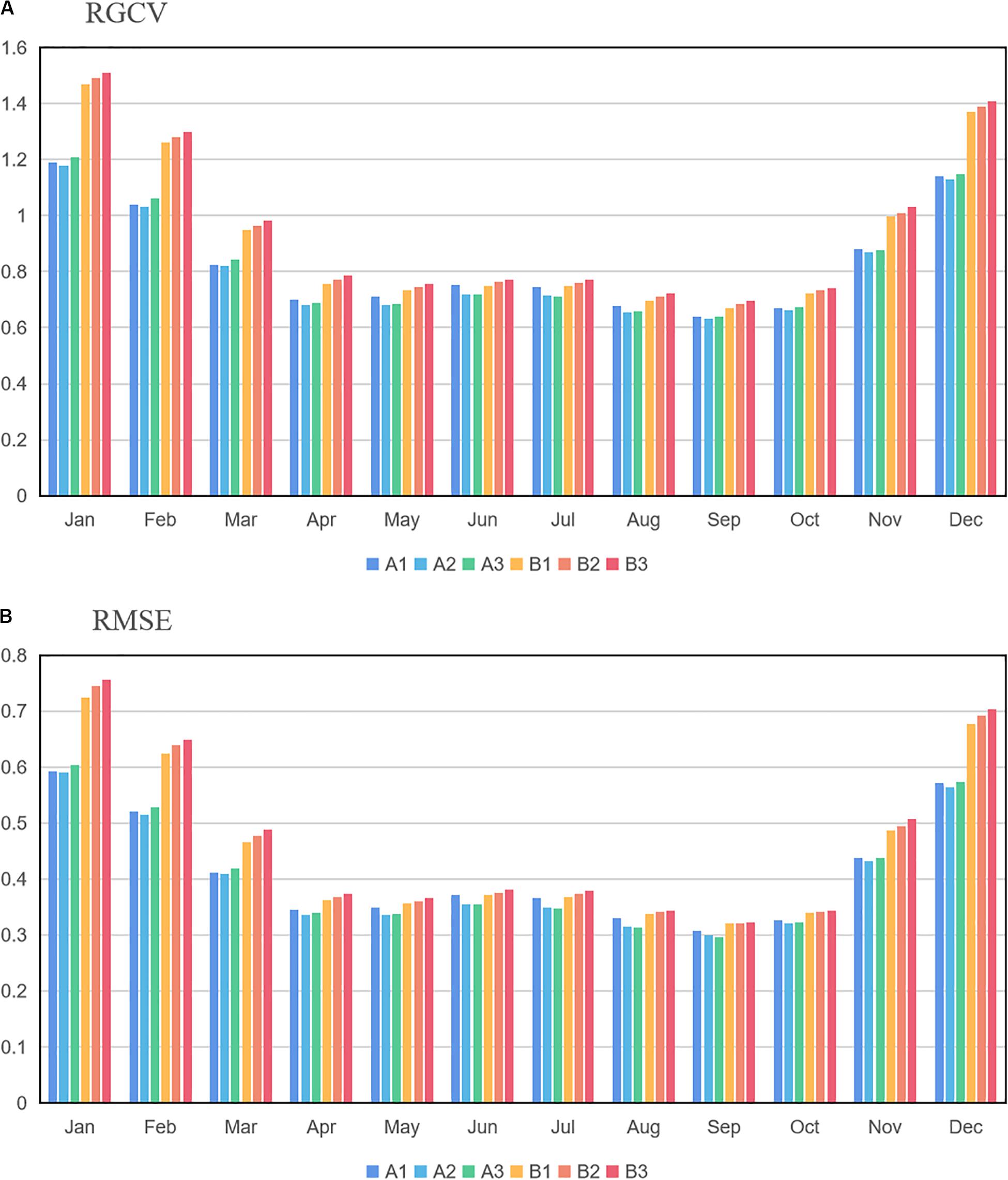
Figure 3. Monthly RGCV (A) and RMSE (B) of the six test experiments (°C).

RMSE is another statistical measure to estimate the degree of dispersion of interpolation errors. Figure 3B shows the RMSE of the six experiments. As seen from the figure, the lowest RMSE occurs in spring and autumn, slightly higher in summer, and highest in winter.

Table 1 shows the annual average RGCV and RMSE for the six test experiments. It is found that both the RGCV and RMSE are lower in group A than that in group B, and the smallest RGCV (0.835°C) and RMSE (0.619°C) appear in experiment A2.

After taking into account the above statistical indices, we decided to take experiment A2 as the preferred scheme to interpolate the climatology temperature, which means to treat the longitude, latitude as well as the elevation as independent variables, and the spline order as 3. It is worth noting that this scheme is just applicable to the data in this study. There may be other better schemes for data from different regions or scales, which need to be analyzed according to the actual situation.

Climatology Interpolation

After the preparation for the input data and model parameter setting, we adopted the ANUSPLIN software to interpolate the gridded temperature climatology over Pan-East Asia. Figure 4 shows the gridded result of the LSAT climatology over the region. The spatial distribution of LSAT climatology is obviously affected by the terrain and latitude. Naturally, the climatological temperature is higher at lower latitudes. The lowest temperature was found at high latitudes in eastern Siberia while the highest temperature was found at low latitudes in India and Indochina. In addition, the temperature climatology decreases with the increasing elevation. The climatological temperature at high altitude areas, such as the Tibet plateau and Mount Tianshan, is significantly lower than that at low altitude areas at the same latitude.

FIGURE 4

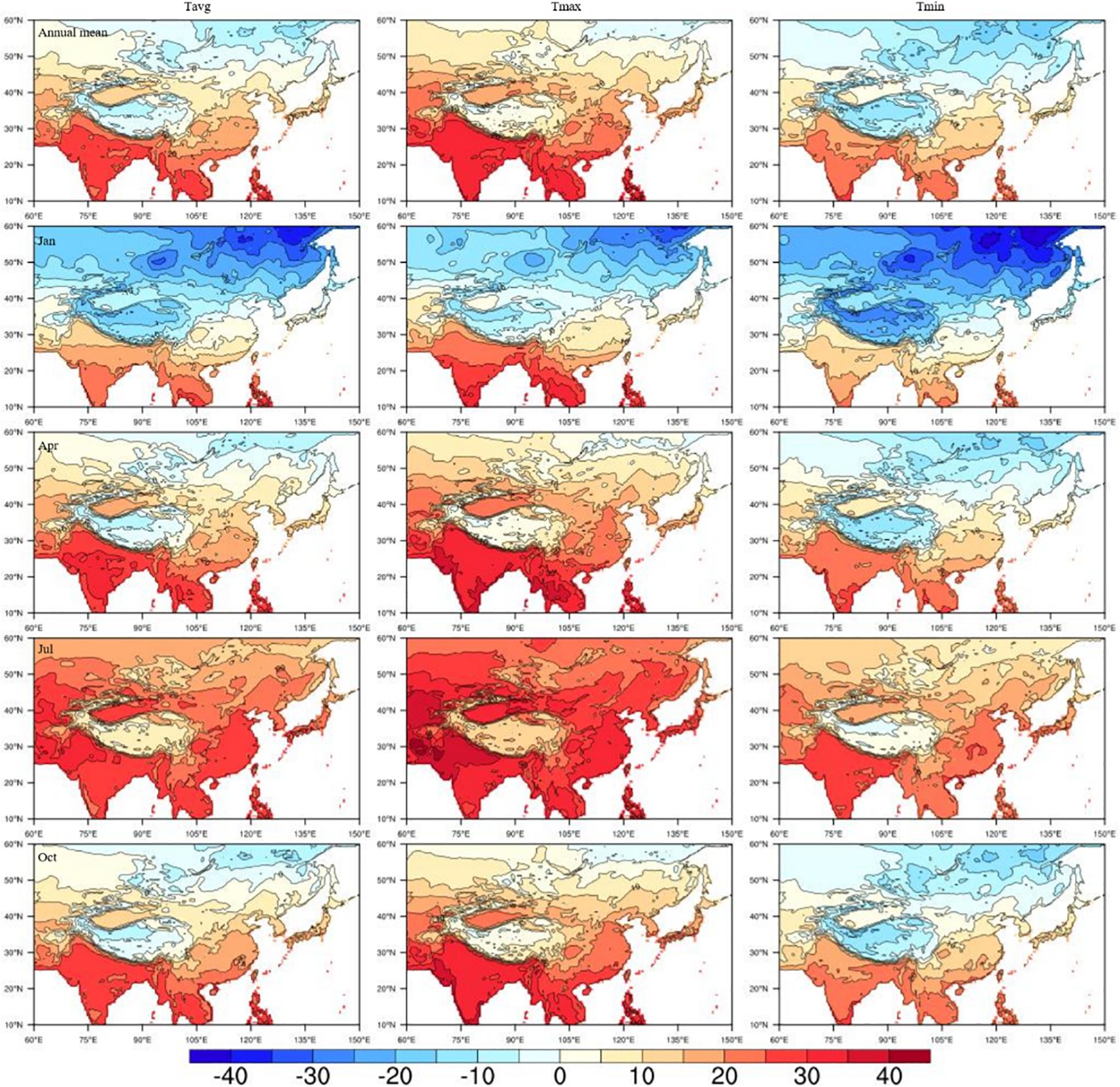
Figure 4. Gridded climatology (°C) of LSAT over eastern Asia for (top to bottom) annual mean and different seasons (presented by January, April, July, and October) of mean, maximum and minimum temperature (left to right).

Interpolation and Validation of LSAT Anomaly

Anomaly Interpolation

In this section, we used the AIDW method to interpolate the monthly anomaly of LSAT over Pan-East Asia during 1900–2018. In order to demonstrate the interpolation effect, four representative years are selected to display the spatial distributions of temperature anomalies (Figure 5): the spatial distribution of the LSAT anomalies of the coldest (1912) and warmest (1948) year before 1950 and the coldest (1969) and warmest (2007) year after 1950.

FIGURE 5

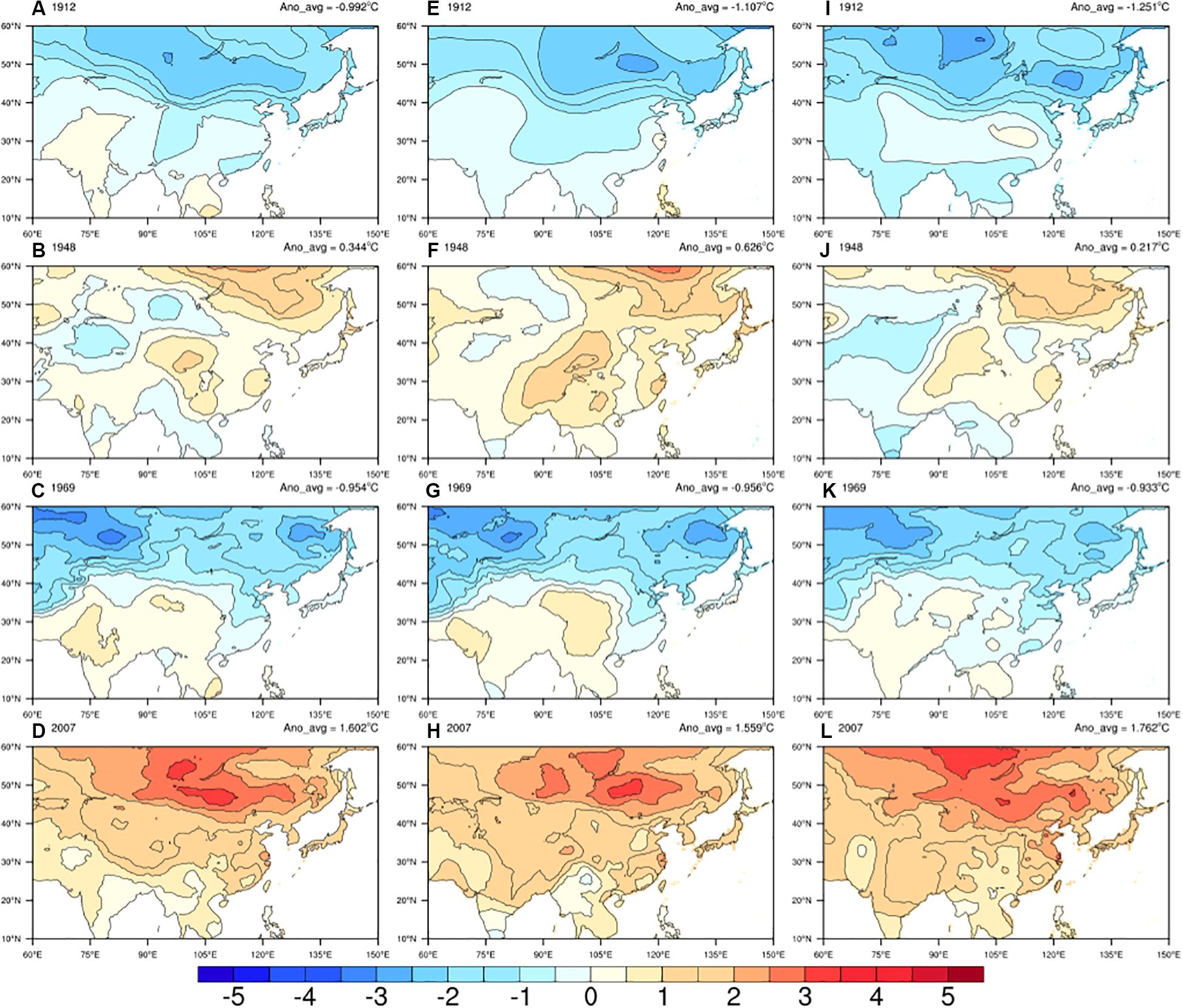
Figure 5. The spatial distribution of the annual anomalies of mean (A–D), maximum (E–H) and minimum (I–L) LSAT (left to right) of the coldest (1912) and warmest (1948) year before 1950s and the coldest (1969) and warmest (2007) year after 1950s.

In the two coldest years (1912 and 1969), the temperature anomalies (relative to 1961–1990 averages) in the high latitude region north of 40°N is generally lower than those in the lower latitude region, and there is very little change before and after 1950s. Differences exist in the detailed distribution of the anomaly in warmest years, in the first half of the 20th century, the LSAT anomaly was not so high (0.34°C) relative to 1961–1990 average even in the warmest year (1948), and the warming center happened at higher latitude (55–60°N). The regional LSAT anomaly increased significantly after entering the second half of the 20th century. It reaches the highest LSAT anomaly (1.6°C) in 2007, and the warming center moved to the lower latitude and was significantly expanded. The annual anomalies of maximum and minimum LSAT perform similarly to those of mean LSAT.

Anomaly Validation

In this case, we used the leave-one-out CV to evaluate the interpolation performance. The RMSE, MAE, and MBE have been calculated to evaluate and analyze the interpolation errors between the estimated and observational LSAT.

Figures 6A–D show the distribution of the RMSE of the LSAT anomaly at each station in four seasons (presented by January, April, July, and October) over Pan-East Asia from 1900 to 2018. Inset figures in the lower right corner is the probability density distribution diagram of RMSE for all stations. The stations with RMSE in the range of below 0.75°C are in the majority, accounting for 67.5, 88.5, 90.1, and 88.7% in each month (January, April, July, and October), respectively. Figures 6B–D show that the spatial distribution and the average of the RMSE is mostly similar between spring, summer, and autumn. The stations with lowest RMSE mainly located in the regions with high station density in eastern China, Japan, and South Korea. Those with higher RMSE are in regions of relatively sparse station density in India, Indo-China Peninsula and Mongolia. The stations with largest RMSE exist mainly in high latitude mountain areas such as Mount Tianshan (around 40–45°N, 75–80°E). The RMSE over the Tibetan Plateau is hard to determine due to the lack of observational station data. The RMSE in winter is larger than those in other seasons, especially on the Tibetan Plateau and regions north of 40°N. The RMSE in winter (January) is about 0.4°C higher than that in other seasons on average. In contrast, the RMSE in the plain regions south of 40°N is just about 0.08°C higher in winter than in other seasons on average. We suspect that this higher noise level may be related to the circulation and front activities in high latitude regions in winter.

FIGURE 6

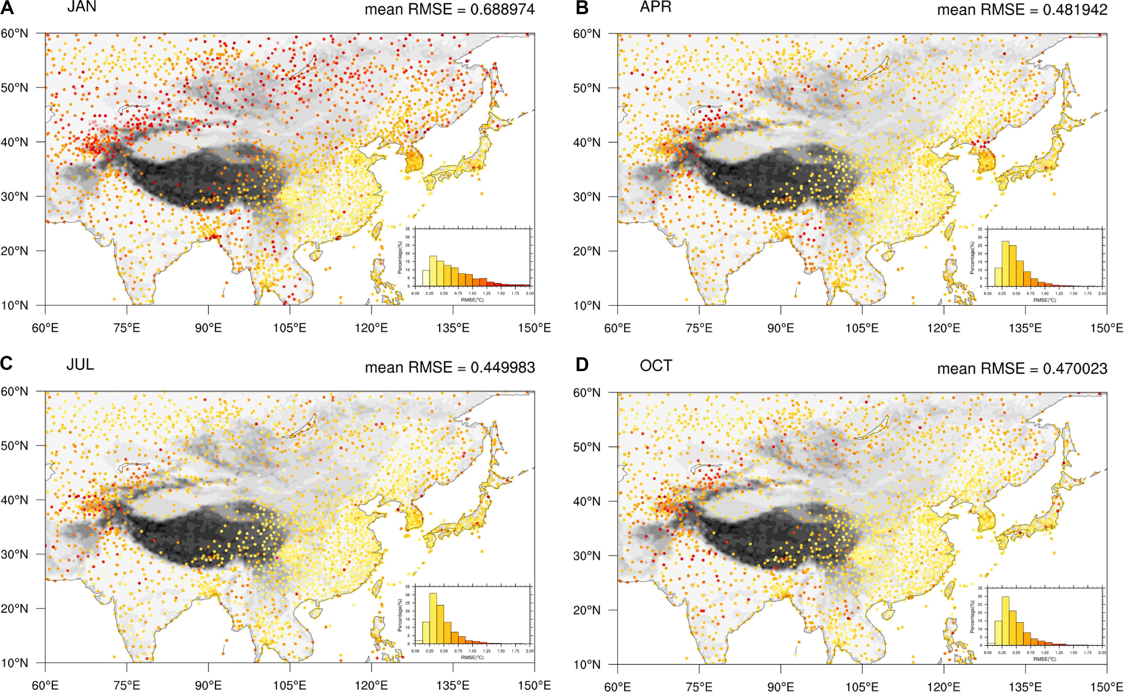
Figure 6. RMSEs of the LSAT anomaly over Pan-East Asian from 1900 to 2018 at each station in 4 months [January (A), April (B), July (C), and October (D)] calculated by leave-one-out cross validation.

Figures 7A–D show the MAEs of the anomaly of LSAT at each station in 4 months (January, April, July, and October) over Pan-East Asia from 1900 to 2018. The magnitude of MAE is smaller than RMSE, but its spatial distribution is very similar to RMSE. In addition, Figure 7 also shows that the MAE is relatively low in general, which means that the systematic error of anomaly temperature generated by the AIDW interpolation model used in this paper is relatively small.

FIGURE 7

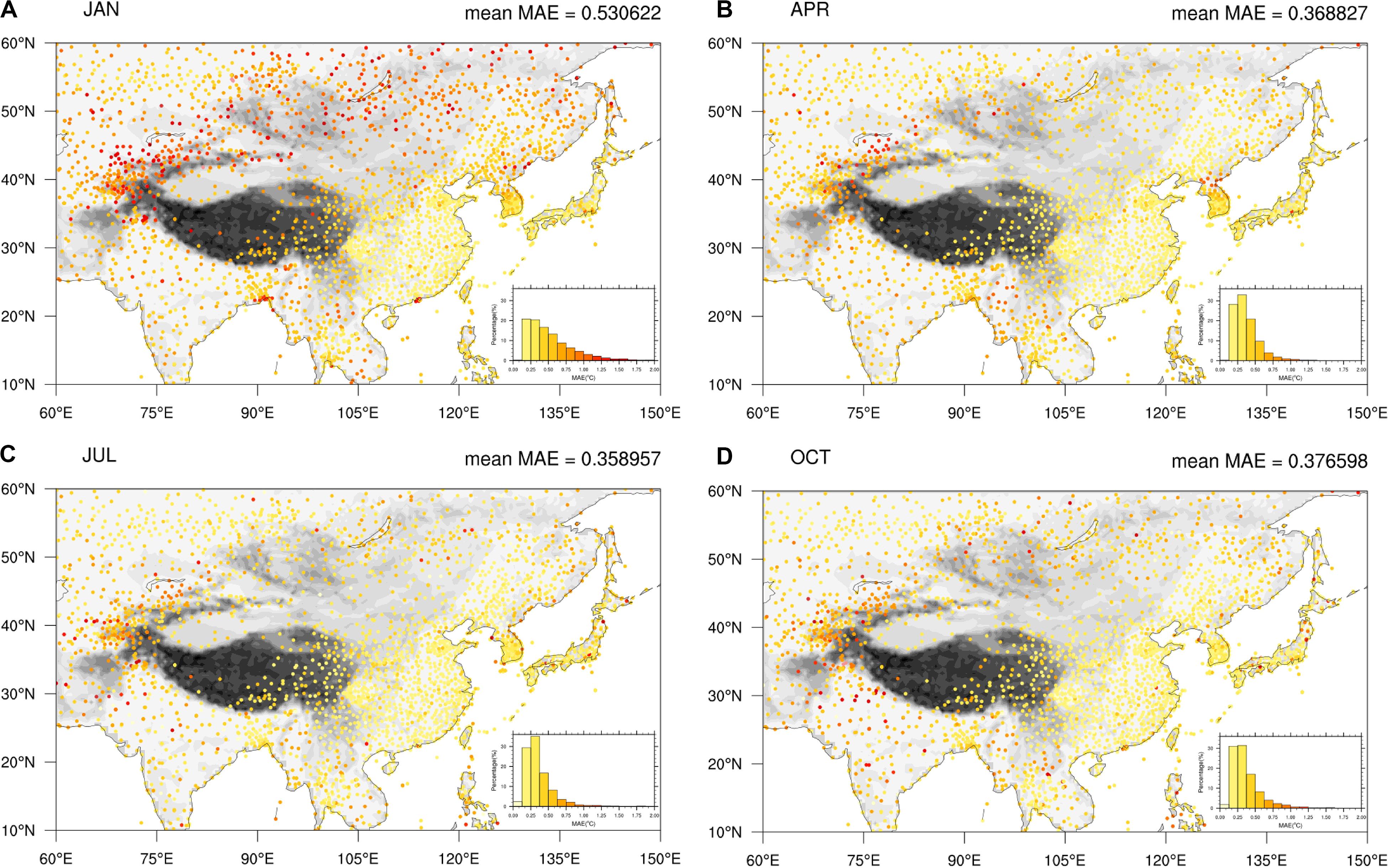
Figure 7. MAEs of the LSAT anomaly over Pan-East Asian from 1900 to 2018 at each station in 4 months [January (A), April (B), July (C), and October (D)] calculated by leave-one-out cross validation.

Figures 8, 9 show the changes of RMSE and MAE of LSAT anomaly during 1900 to 2018 for the 4 months (January, April, July, and October), respectively. Although the 4 months exhibit short-term fluctuations, their long term variations are very similar. Before the 1950s, both of RMSE and MAE are relatively larger and gradually decrease with time. They decreased rapidly and then rose slowly after 1950s (with the change of the stations number), but basically remained lower than those before 1950s. The evolution of RMSE and MAE is strongly related to the change in the station numbers: more station observations correspond to a denser station distribution and hence lower error RMSE and MAE. Similarly, both of the RMSE and MAE in winter are larger than those in other seasons. This also shows that we need more stations in January to reduce the error to that of the other times of the year.

FIGURE 8

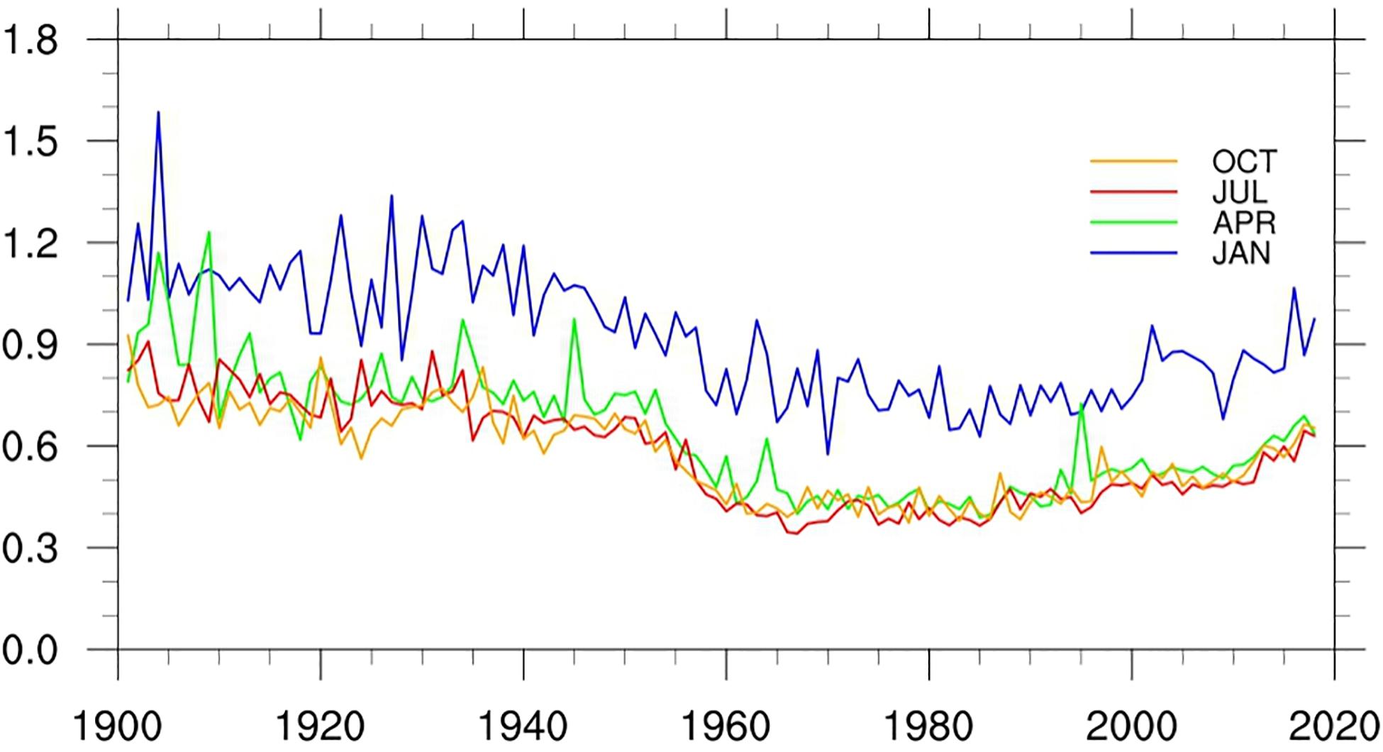
Figure 8. Mean RMSEs of the LSAT anomaly from 1900 to 2018 for 4 months (January, April, July, and October).

FIGURE 9

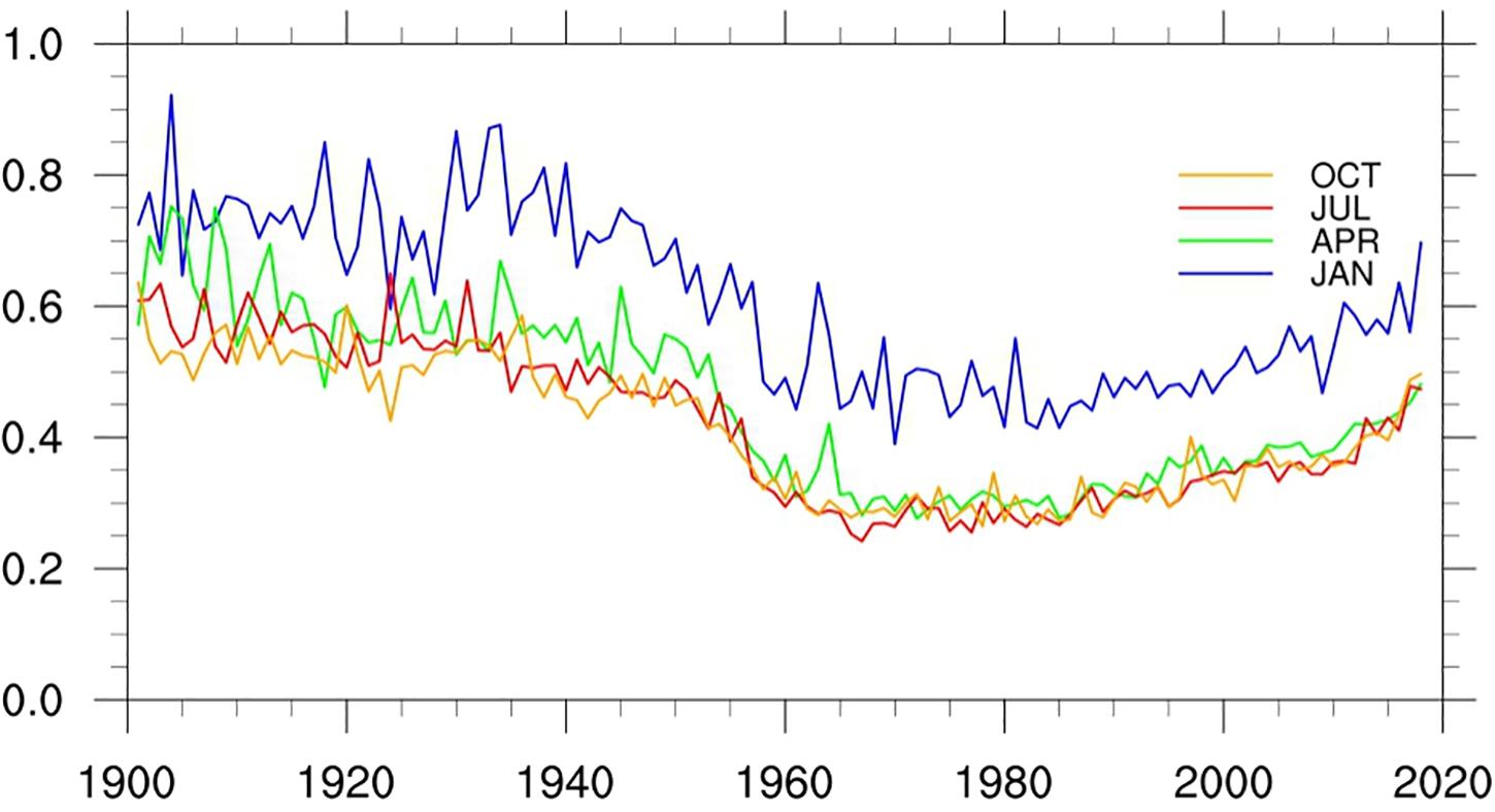
Figure 9. Mean MAEs of the LSAT anomaly from 1900 to 2018 for 4 months (January, April, July, and October).

Regional LSAT Warming Trends Analysis

In order to investigate the long-term climate change trend reflected by the new interpolation high resolution dataset, we calculated the long term regional C-LSAT high resolution (C-LSAT HR) anomaly time series over the Pan-East Asia and compared it with the newly released high resolution CRU TS4 (Harris et al., 2020) dataset. Table 2 shows the difference of the high resolution gridded dataset between CRU TS and C-LSAT HR over Pan East Asia.

TABLE 2

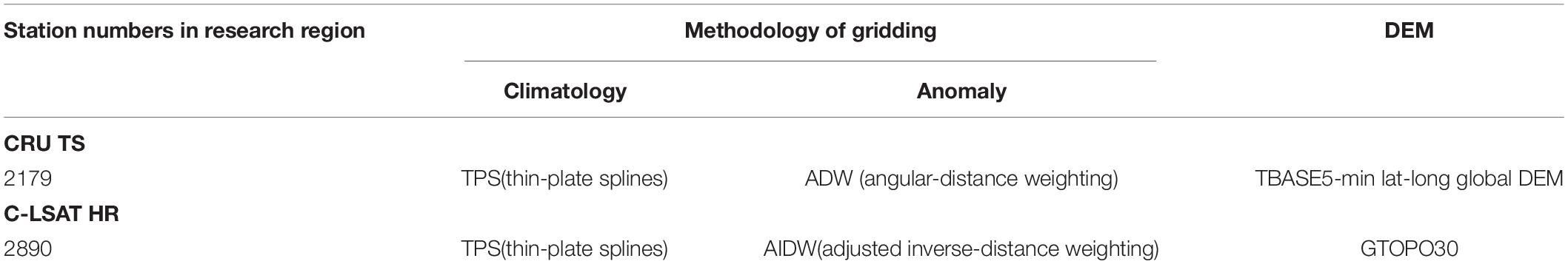
Table 2. The comparison of the high resolution gridded dataset derived from CRU TS and C-LSAT HR.

Figure 10 shows the time series of the annual surface air temperature anomaly over Pan-East Asia from the high-resolution dataset obtained by AIDW (C-LSAT HR) and the high-resolution estimation of CRU data (CRU TS) in the same region, respectively. The linear trends with 5% significant range are listed in Table 3.

FIGURE 10

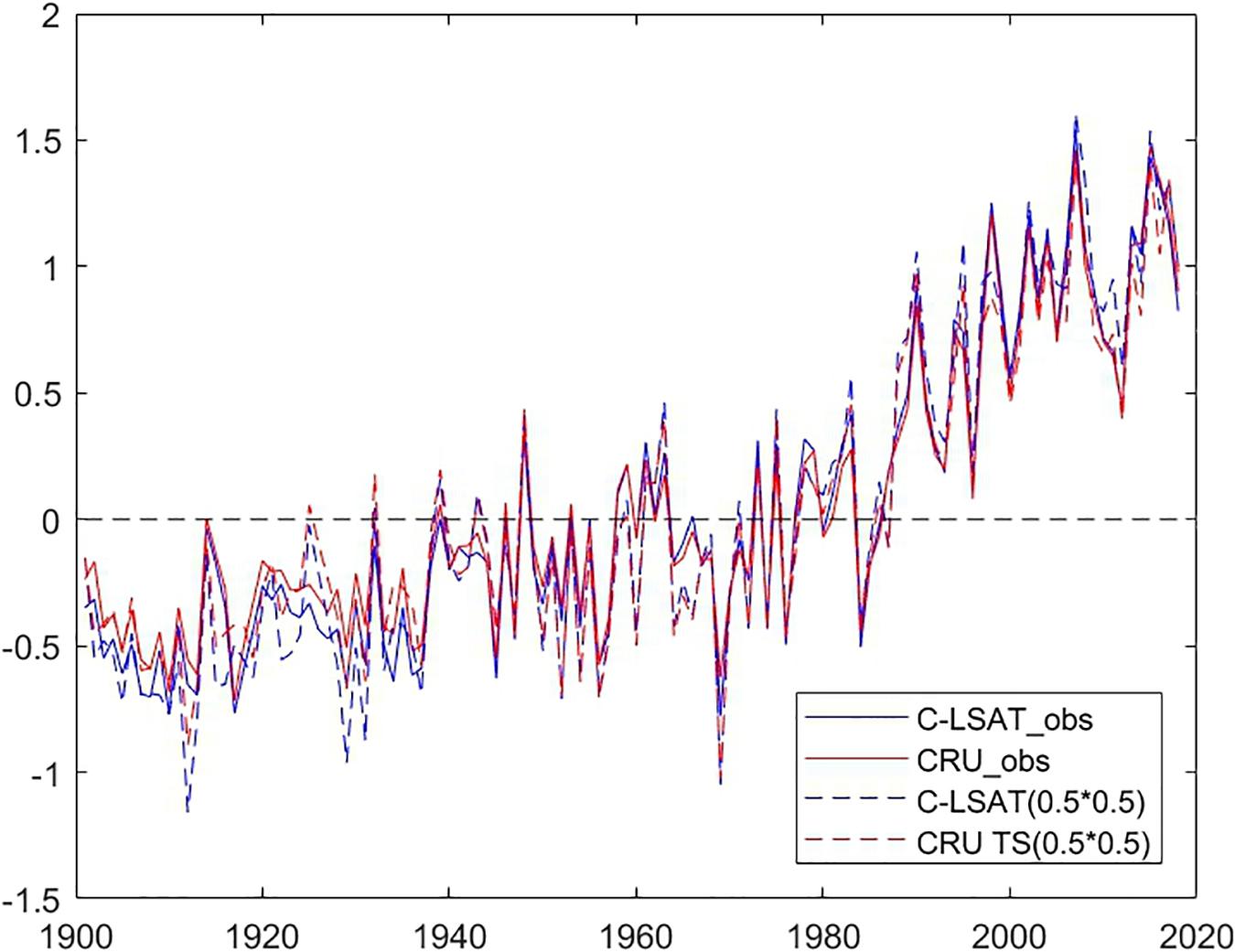
Figure 10. The time series of the annual LAST anomaly in Pan-East Asian area from C-LSAT HR (blue) and CRU TS4 (red), including observed (dashed), and estimated (solid) data.

TABLE 3

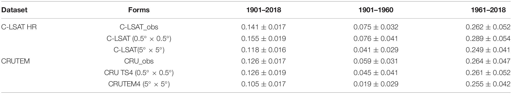
Table 3. Warming trends (°C 10a^–1) and their uncertainty at 95% confidence level of annual LSAT anomaly from observation and gridded datasets over Pan-East Asian.

From Table 3 and Figure 10, it is noticed that the variations of the two annual mean LSAT anomalies are overall close to each other, except for slight difference in the warming trends between two datasets. The trend derived from the C-LSAT HR (0.5 × 0.5) (0.155 ± 0.019°C/10 years) is slightly larger than that of CRU TS4 (0.126 ± 0.019°C/10 years) for the whole period of 1901–2018. It is similar for the linear trends comparison during different periods. From the early 20th century to the early 1960s, the trend of annual average temperature is relatively low (0.076 ± 0.041°C/10 years for AIDW and 0.044 ± 0.041°C/10 years for CRU TS4). The linear trend of annual LSAT anomaly rose rapidly after the mid-1960s (0.289 ± 0.054°C/10 years for AIDW and 0.261 ± 0.052°C/10 years for CRU TS4). Further comparison indicates that this agrees well with the result calculated by the arithmetic average trend of all the stations, which also shows the interpolation process performs well.

Finally, from Table 3, no matter for C-LSAT or CRU TS gridded datasets (both 0.5° × 0.5° and 5° × 5° resolution), the trends calculated by low resolution datasets (5° × 5° resolution, Yun et al., 2019) are lower than those by higher resolution datasets (0.5° × 0.5° resolution). This may be due to the fact that the high-resolution data sets emphasize more on the amplification effect of local warming in some areas in high altitudes (Li et al., 2009; Pepin et al., 2015) or in regions with severe drought (Huang et al., 2016) where there are no actual observation stations especially when the stations are relatively scarce (mostly in the Tibet Plateau and large desert areas) before 1960.

Conclusion

In this paper, we first split the land surface air temperature from C-LSAT2.0 into climatology and anomaly data, and then interpolate them into a 0.5° × 0.5° grid datasets, respectively. Finally they are combined into a new monthly high-resolution LSAT grid data set for the period of 1900–2018 over Pan-East Asia. The validation of the dataset shows that the interpolated dataset is of good accuracy in both climatology and the LSAT anomaly variations.

The climatology data is interpolated by thin-plate splines (TPS) method using station LSAT data from C-LSAT2.0 and elevation information (DEM) from GTOPO30 as the input data to the ANUSPLIN software. We found that the interpolation scheme performs best when the longitude, latitude and elevation are all used as independent variables, and the spline order is set to 3. Under this situation, the lowest RGCV and RMSE are achieved.

The LSAT anomaly data is interpolated by an AIDW method. The gridded LSAT anomaly data errors are evaluated by leave-one-out CV. The spatial distribution characteristic of RMSE and MAE are closely correlated with the station density in both temporal and special perspective. The low RMSE mainly occurs in the regions with high station density areas in eastern China, Japan, and South Korea. The RMSE further decreases with the increase of the station numbers during the period of 1900–2018. In addition, the RMSE and MAE in winter are much larger than those in other seasons, which indicate a clear seasonal difference. This may be related to the more active cold air activities in the high latitudes regions in winter and the temperature anomalies in winter being more controlled by advection when the winds are strong than the other seasons.

In addition, we evaluated the long term LSAT change trend during the period of 1901–2018, 1901–1960, and 1961–2018, respectively with the newly interpolated high resolution dataset, and compared the results with those derived from CRU TS4 dataset. The LSAT anomaly series during 1900–2018 derived in this paper and from CRU TS4 are generally consistent with each other, while the linear warming trends have slight differences. The trend derived from newly dataset is a bit larger than those from the latter dataset in different time periods of 1901–2018, 1901–1960, and 1961–2018, respectively. Based on above analysis, the dataset developed in this paper is proved to be a useful tool in the regional climate and climate change detection, monitoring and validation of model output.

The future plan is developing a global higher resolution LSAT dataset based on the whole C-LSAT (C-LSAT HR). This is a part of global dataset, we found it is relatively mature in pan East Asia. We are going to apply this gridding and validation method to other sub-regions over the world, and focus on the gridded data integration of regions and the overall quality of the global gridded dataset. Once the development of this global high-resolution LSAT dataset is completed, the dataset will be available to the public (for free) in near future. The gridding and validation method used in this study is also helpful for other similar research, such as gridding of precipitation, wind speed or other meteorological elements in monthly, daily or even higher temporal scale, which is also another part of our future research direction.

Data Availability Statement

The raw data supporting the conclusions of this article will be made available by the authors, without undue reservation, to any qualified researcher.

Author Contributions

JC analyzed the data. QL put forward the idea. QL and JC wrote the manuscript. All authors revised the manuscript.

Funding

This study was supported by the National Key R&D Program of China (Grant: 2017YFC1502301 and 2018YFC1507705) and the Natural Science Foundation of China (Grant: 41975105).

Conflict of Interest

The authors declare that the research was conducted in the absence of any commercial or financial relationships that could be construed as a potential conflict of interest.

Acknowledgments

The authors thank the editor and the reviewers for their constructive suggestions/comments in the initial reviews.

References

Callendar, G. S. (1938). The artificial production of carbon dioxide and its influence on temperature. Q. J. R. Meteorol. Soc. 64, 223–240. doi: 10.1002/qj.49706427503

CrossRef Full Text | Google Scholar

Callendar, G. S. (1961). Temperature fluctuations and trends over the Earth. Q. J.R. Meteorol. Soc. 87, 1–12. doi: 10.1002/qj.49708737102

CrossRef Full Text | Google Scholar

Daly, C., Halbleib, M., Smith, J. I., Gibson, W. P., Doggett, M. K., Taylor, G. H., et al. (2008). Physiographically sensitive mapping of climatological temperature and precipitation across the conterminous united states. Int. J. Climatol. 28, 2031–2064. doi: 10.1002/joc.1688

CrossRef Full Text | Google Scholar

Daly, C., Neilson, R. P., and Phillips, D. L. (1994). A statistical-topographic model for mapping climatological precipitation over mountainous terrain. J. Appl. Meteor. 33, 140–158. doi: 10.1175/1520-0450(1994)033<0140:astmfm>2.0.co;2

CrossRef Full Text | Google Scholar

Duan, P., Sheng, Y., Li, J., Lv, H., and Zhang, S. (2014). Adaptive idw interpolation method and its application in the temperature field. Geograph. Res. 196, 31–38.

Google Scholar

Farr, T. G., Rosen, P. A., Caro, E., Crippen, R., Duren, R., Hensley, S., et al. (2007). The shuttle radar topography mission. Rev. Geophys. 45:RG2004. doi: 10.1029/2005RG000183

CrossRef Full Text | Google Scholar

Fick, S. E., and Hijmans, R. J. (2017). WorldClim 2: new 1-km spatial resolution climate surfaces for global land areas. Int. J. Climatol. 37, 4302–4315. doi: 10.1002/joc.5086

CrossRef Full Text | Google Scholar

Hansen, J., Ruedy, R., Glascoe, J., and Sato, M. (1999). GISS analysis of surface temperature change. J. Geophys. Res. 104, 30997–31022. doi: 10.1029/1999jd900835

CrossRef Full Text | Google Scholar

Harris, I., Osborn, T. J., Jones, P., and Lister, D. (2020). Version 4 of the CRU TS monthly high-resolution gridded multivariate climate dataset. Sci. Data 7:109.

Google Scholar

Hawkins, E. D., and Jones, P. D. (2013). Notes and Correspondence On increasing global temperatures: 75 years after Callendar. Q. J. R. Meteorol. Soc. 139, 1961–1963. doi: 10.1002/qj.2178

CrossRef Full Text | Google Scholar

Haylock, M. R., Hofstra, N., Klein Tank, A. M. G., Klok, E. J., Jones, P. D., and New, M. (2008). A European daily high-resolution gridded data set of surface temperature and precipitation for 1950–2006. J. Geophys. Res. 113:D20119.

Google Scholar

Hijmans, R. J., Cameron, S. E., Parra, J. L., Jones, P. G., and Jarvis, A. (2005). Very high resolution interpolated climate surfaces for global land areas. Int. J. Climatol. 25, 1965–1978. doi: 10.1002/joc.1276

CrossRef Full Text | Google Scholar

Hong, Y., Nix, H. A., Hutchinsonb, M. F., and Booth, T. H. (2005). Spatial interpolation of monthly mean climate data for china. Int. J. Climatol. 25, 1369–1379. doi: 10.1002/joc.1187

CrossRef Full Text | Google Scholar

Huang, J., Yu, H., Guan, X., Wang, G., and Guo, R. (2016). Accelerated dryland expansion under climate change. Nat. Clim. Change 6, 166–171. doi: 10.1038/nclimate2837

CrossRef Full Text | Google Scholar

Huang, W., Liu, C., Cao, J., Chen, J., and Feng, S. (2020). Changes of hydroclimatic patterns in China in the present day and future. Sci. Bull. 65, 1061–1063. doi: 10.1016/j.scib.2020.03.033

CrossRef Full Text | Google Scholar

Hutchinson, M. F. (1991). The application of thin plate smoothing splines to continent-wide data assimilation. Melbourne Bureau Meteorol. Res. Rep. 01, 104–113.

Google Scholar

Hutchinson, M. F., and Xu, T. (2013). Anusplin version 4.4 user guide.

Google Scholar

Jones, P. D., and Briffa, K. R. (1992). Global surface air temperature variations during the twentieth century: part I, spatial temporal and seasonal details. Holocene 2, 165–179. doi: 10.1177/095968369200200208

CrossRef Full Text | Google Scholar

Köppen, W. (1931). Grundriss der Klimakunde. (Zweite, verbesserte Auflage der Klimate der Erde.). Berlin: Walter de Gruyter & Co.

Google Scholar

Li, Q., and Li, W. (2007). Construction of the gridded historic temperature dataset over china during the recent half century. Acta Meteorol. Sin. 65, 293–300.

Google Scholar

Li, Q., Li, W., Si, P., Gao, X., Dong, W., Jones, P., et al. (2009). Assessment of surface air warming in northeast China, with emphasis on the impacts of urbanization. Theor. Appl. Climatol. 99, 469–478. doi: 10.1007/s00704-009-0155-4

CrossRef Full Text | Google Scholar

Li, Q., Sun, W., Huang, B., Dong, W., Wang, X., Zhai, P., et al. (2020). Consistence of global warming trends strengthened since 1880s. Sci. Bull. 65, 1709–1712. doi: 10.1016/j.scib.2020.06.009

CrossRef Full Text | Google Scholar

Li, Q., Zhang, L., Xu, W., Zhou, T., Wang, J., Zhai, P., et al. (2017). Comparisons of time series of annual mean surface air temperature for China since the 1900s:Observation, Model simulation and extended reanalysis. Bull. Am. Meteor. Soc. 98, 699–711. doi: 10.1175/BAMS-D-16-0092.1

CrossRef Full Text | Google Scholar

Li, W., Li, Q., and Jiang, Z. (2007). Discussion on feasibility of gridding the historic temperature data in China with kriging method. J. Nanjing Instit. Meteorol. 30, 246–252.

Google Scholar

Ma, L., and Li, Y. (2006). Study on accuracy of GTOP030 and srtm dem - a case study of tibet. Bull. Soil Water Conserv. 5, 71–74. doi: 10.2747/1548-1603.49.1.71

CrossRef Full Text | Google Scholar

New, M., Hulme, M., and Jones, P. (1999a). Representing twentieth-century space-time climate variability. Part I: development of a 1961-90 mean monthly terrestrial climatology. J. Clim. 12, 829–856. doi: 10.1175/1520-0442(1999)012<0829:rtcstc>2.0.co;2

CrossRef Full Text | Google Scholar

New, M., Hulme, M., and Jones, P. (1999b). Representing twentieth-century space-time climate variability. Part II: development of 1901-96 monthly grids of terrestrial surface climate. J. Clim. 13, 2217–2238. doi: 10.1175/1520-0442(2000)013<2217:rtcstc>2.0.co;2

CrossRef Full Text | Google Scholar

Nynke, H., Malcolm, H., Mark, N., and Phil, J. (2009). Testing E-OBS European high-resolution gridded dataset of daily precipitation and surface temperature. J. Geophys. Res. 114:D21101.

Google Scholar

Peng, S., Ding, Y., Liu, W., and Li, Z. (2019). 1km monthly temperature and precipitation dataset for China from 1901 to 2017. Earth Syst. Sci. Data 11, 1931–1946. doi: 10.5194/essd-11-1931-2019

CrossRef Full Text | Google Scholar

Pepin, N. C., Bradly, R. S., Diaz, H. F., Baraer, M., Caceres, E. B., Forsythe, N., et al. (2015). Elevation-dependent warming in mountain regions of the world. Nat. Clim. Chang. 5, 424–430. doi: 10.1038/nclimate2563

CrossRef Full Text | Google Scholar

Peterson, T. C., and Vose, R. S. (1997). An overview of the global historical climatology network temperature database. Bull. Am. Meteorol. Soc. 78, 2837–2849. doi: 10.1175/1520-0477(1997)078<2837:aootgh>2.0.co;2

CrossRef Full Text | Google Scholar

Price, D. T., McKenney, D. W., Papadopol, P., Logan, T., and Hutchinson, M. F. (2004). “High resolution future scenario climate data for North America,” in Proceedings of the 26th Conference on Agricultural and Forest Meteorology of American Meteorological Society, Boston, MA.

Google Scholar

Rohde, R., Muller, R., Jacobsen, R., Perlmutter, S., Rosenfeld, A., Wurtele, J., et al. (2013). Berkeley Earth Temperature averaging process. Geoinform. Geostat. Overview 1:2.

Google Scholar

Sinha, S. K., Narkhedkar, S. G., and Mitra, A. K. (2006). Bares objective analysis scheme of daily rainfall over Maharashtra (India) on a mesoscale grid. Atmosfera 19, 109–126.

Google Scholar

Van den Besselaar, E. J. M., Van der Schrier, G., Cornes, R. C., Iqbal, A. S., and Tank, A. M. G. K. (2017). SA-OBS: a daily gridded surface temperature and precipitation dataset for Southeast Asia. J. Clim. 30, 5151–5165. doi: 10.1175/jcli-d-16-0575.1

CrossRef Full Text | Google Scholar

Wahba, G., and Wendelberger, J. (1980). Some new mathematical methods for variational objective analysis using splines and cross-validation. Mon. Weather Rev. 108, 1122–1145. doi: 10.1175/1520-0493(1980)108<1122:snmmfv>2.0.co;2

CrossRef Full Text | Google Scholar

Wu, J., and Gao, X. (2013). A gridded daily observation dataset over China region and comparison with the other datasets. Chin. J. Geophys. 56, 1102–1111.

Google Scholar

Xie, P., Yatagai, A., Chen, M., Hayasaka, T., Fukushima, Y., Liu, C., et al. (2007). A gauge-based analysis of daily precipitation over East Asia. J. Hydrol. 8, 607–626. doi: 10.1175/jhm583.1

CrossRef Full Text | Google Scholar

Xu, C., Wang, J., and Li, Q. (2018). A new method for temperatures spatial interpolation based on sparse historical stations. J. Clim. 31, 1757–1770. doi: 10.1175/jcli-d-17-0150.1

CrossRef Full Text | Google Scholar

Xu, W., Li, Q., Jones, P., Wang, X. L., Trewin, B., Yang, S., et al. (2018). A new integrated and homogenized global monthly land surface air temperature dataset for the period since 1900. Clim. Dyn. 50, 2513–2536. doi: 10.1007/s00382-017-3755-1

CrossRef Full Text | Google Scholar

Xu, Y., Gao, X., Shen, Y., Xu, C., Shi, Y., and Giorgi, F. (2009). A daily temperature dataset over China and its application in validating a RCM simulation. Adv. Atmos. Sci. 26, 763–772. doi: 10.1007/s00376-009-9029-z

CrossRef Full Text | Google Scholar

Xu, Y., Zhao, P., Si, D., Cao, L., Wu, X., Zhao, Y., et al. (2020). Development and preliminary application of a gridded surface air temperature homogenized dataset for China. Theor. Appl. Climatol. 139, 505–516. doi: 10.1007/s00704-019-02972-z

CrossRef Full Text | Google Scholar

Yatagai, A., Arakawa, O., Kamiguchi, K., Kawamoto, H., Nodzu, M., and Hamada, A. (2009). A 44-year daily gridded precipitation dataset for Asia based on a dense network of rain gauges. SOLA 5, 137–140. doi: 10.2151/sola.2009-035

PubMed Abstract | CrossRef Full Text | Google Scholar

Yun, X., Huang, B., Cheng, J., Xu, W., Qiao, S., and Li, Q. (2019). A new merge of global surface temperature datasets since the start of the 20th Century. Earth Syst. Sci. Data 11, 1629–1643. doi: 10.5194/essd-11-1629-2019

CrossRef Full Text | Google Scholar