Human Population Density is a Poor Predictor of Debris in the Environment

Introduction

The impacts from marine plastic pollution to wildlife, human health, and the economy are well documented (Gall and Thompson, 2015; Beaumont et al., 2019) and are likely to continue to increase as global plastic production rises (Geyer et al., 2017). Because an estimated 80% of marine plastic pollution has land-based origins (Derraik, 2002), the most efficient way to address the problem is by stopping plastic waste leakage from land to the sea. Plastics typically enter the ocean from land as mismanaged waste transported via rivers or wind (Kershaw and Rochman, 2015), though local human deposition in coastal areas also contributes (Hardesty et al., 2016). While debris on land is found ubiquitously and has been reported from the most remote to the most densely populated corners of the earth, it is not equally distributed (Barnes et al., 2009; Martins et al., 2020; Napper et al., 2020).

Many studies have investigated debris at local or regional scales (e.g., Wessel et al., 2019; Miladinova et al., 2020; Vidyasakar et al., 2020) These studies are predominately carried out along the coastal margin (Serra-Gonçalves et al., 2019) though studies along rivers and at river outlets are becoming more common (e.g., Battulga et al., 2019; Cordova and Nurhati, 2019; Van Calcar and Van Emmerik, 2019). However, these empirical studies are, by necessity, restricted to a limited area, so in order to understand debris distribution on a broader scale, modeling and predictions are critical. For the most part, these studies use globally available data sources as proxies for the amount of mismanaged waste entering the environment (but see Lebreton et al., 2017).

Jambeck and colleagues used global data sets to predict mismanaged waste and calculated that an estimated 4.8–12.7 million MT of plastic entered the ocean in 2010 (2015). They hypothesized that population size and the quality of waste management systems in a country were most important predictors of the amount of debris lost to the marine environment. Lebreton et al. (2017) similarly relied predominately on global estimates of population density and mismanaged plastic waste, but additionally factored in runoff to estimated that between 1.15 and 2.41 MT of plastic is transported to the ocean via rivers. This research also relied on published empirical studies to calibrate the models. Models of floating plastic distribution in the ocean used coastal population density to seed the models (e.g., Van Sebille et al., 2012; Van Sebille, 2014), with (in instances) the addition of impervious surface area (Lebreton et al., 2012) and mismanaged waste (Van Sebille et al., 2015).

More recent studies have acknowledged the fact that mismanaged waste varies not only with population density, but also with factors such as socio-economic status (Borrelle et al., 2020; Lau et al., 2020). Gross Domestic Product (GDP) is positively correlated with reported per capita waste generation, but negatively correlated with the proportion of mismanaged waste, and these relationships can vary between rural and urban areas (Lebreton and Andrady, 2019).

If we are to make accurate predictions, it is critical to test the foundational assumptions that are being made when modeling waste leakage. To date, studies have predominately used global population density estimates without the addition of empirical data, and many of these studies have presumed that population density is an adequate proxy for debris leakage (e.g., Van Sebille et al., 2012). To test these assumptions, we gathered empirical data on debris in the environment in 7 countries/territories (hereafter referred to as countries for simplicity): mainland China, Kenya, South Africa, South Korea, Sri Lanka, Taiwan, and Vietnam. We asked three key questions:

1) What drives the distribution of debris in inland areas?

2) How similar (or different) are these drivers among the seven countries studied?

3) Do models based on population density accurately represent debris observed in the local environment?

To address these questions we assessed a number of potential drivers, including land use, survey type, infrastructure, environmental and socio-economic factors, local population density, and site level information such as steepness and vegetation height (Table 1).

TABLE 1

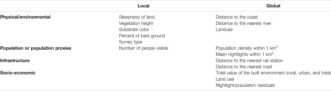
TABLE 1. Local (recorded at site or transect level), and global (determined from global GIS layers) covariates investigated in the study.

Materials and Methods

What Drives the Distribution of Debris in Inland Areas?

This research was undertaken as part of the CSIRO global plastics losses project (https://research.csiro.au/marinedebris/projects/globalplasticsleakageproject/), which is aimed at understanding the amount of plastic that is lost from land to the marine environment. The goal is to use empirical data to quantify and better understand debris leakage rates globally, based on locally collected data across an array of countries. We selected countries based on a combination of factors, including the country’s ranking in estimated mismanaged waste generated annually (per Jambeck et al., 2015). Between 2017–2019 we worked with local partners in each country to select an urban area within a major watershed. The urban areas selected were Shanghai, China; Mombasa, Kenya; Capetown, South Africa; Yeongsan, South Korea; Negombo/Colombo, Sri Lanka; Kaohsiung, Taiwan, and Haiphong, Vietnam. Inland survey sites were then chosen within a 200 km radius of the central point (with the exception of Shanghai, China, where sites were chosen within 100 km due to excessively long travel time between sites). Sites were selected using a stratified random sampling design, taking into account a variety of environmental and socio-economic factors [population density, distance to infrastructure (roads and rail), distance to coast and river, proxies for socio-economic status, and land use]. For each country we pre-selected approximately 40 inland sites, but due to accessibility constraints and the variability in capacity of our local partners, the total number of sites surveyed varied between 23 and 47 (Table 2).

TABLE 2

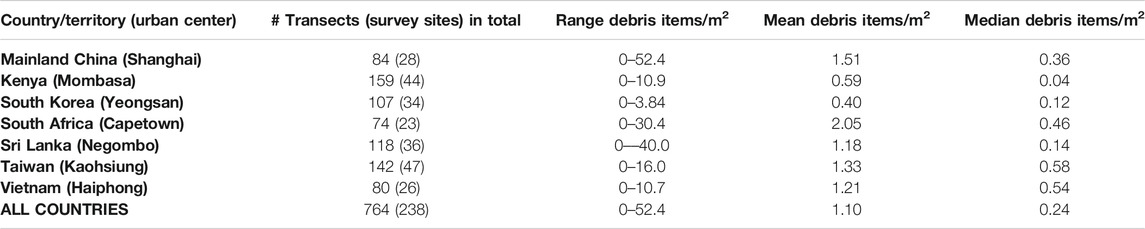
TABLE 2. Range, mean, and median items per meter squared found on inland surveys in each country/territory.

At each site we conducted between 3–6 transects of 25 m², distributed in proportion to the site uses present within 200 m of the central site point (e.g., walkways, natural vegetation, roadways, etc.). Transects were usually 12.5 m × 2 m, except in the case of roadsides, where they were 25 m × 1 m to ensure the safety of the participants. Observers walked the length of the transect, and categorized any anthropogenic debris within the transect that could be seen from standing height. Debris was placed into one of 84 categories, labeled as either fragment or whole (for a complete methodology, see Schuyler et al., 2018b). At each transect, data were also collected on local conditions that could influence the amount of debris found, including the number of people visible at the site, the steepness of the land, the height of the vegetation, substrate color (dark/light), and percent of bare ground in the transect. Both the methods for the survey as well as the local variables to consider were selected based on previous published studies conducted at large scales (Hardesty et al., 2017a; Hardesty et al., 2017c).

Because one of the goals of this project is to estimate the amount of debris leakage on a global scale, we identified covariates for which global datasets existed, that might influence debris levels on a larger scale. In our previous work, land use, infrastructure, and socio-economic factors were among the most important influencers of debris levels (Hardesty et al., 2016). We identified the following environmental and socio-economic variables at each site: population density within 1km², total value of the built environment (rural, urban, and total) identified from the United Nations Global Exposure dataset (GAR15) (UNISDR, 2015), distance to the coast, distance to the nearest rail line, road, and river, mean nightlights within 1 km², and land use. We wanted to incorporate a globally available, socio-economic GIS layer at the finest resolution possible in our analysis, so we explored two potential options. While most socio-economic indicators are national, the GAR15 dataset, developed for assessing economic risk from disasters, is one of the only socio-economic datasets with near-global coverage and sub-national resolution. GAR-15 includes several indicators, including the value of the urban environment, the value of the rural environment, and the total value of assets in a given area, all of which we included in our analyses. Our second option was to use the relationship between lighting at night and population density. In general, the higher the population density, the more nightlights you would expect in a given area. However, in areas with higher income or resources, we would assume a disproportionally higher level of lights than would be predicted by population density alone. Therefore, we used the residual deviation around the linear relationship of nightlights regressed on population density as a second proxy for socio-economic status.

We combined the data from all seven and used model selection on generalized additive models (GAMs) with a Tweedie distribution (mgcv package) in the R statistical environment to find the models with the lowest AIC score (Burnham and Anderson, 2002; Wood, 2011; Bartoń, 2018; R Core Team, 2018). We chose GAMs so that we could experiment with smooths of different factors, though ultimately we settled on parametric terms to be able to predict debris outside of our study area. We used a Tweedie distribution because debris is measured as count data, and the distribution gives the flexibility for the model to range between gamma to Poisson. Because there were a number of factors that could potentially influence the debris in the environment, we used dredge (MuMin package) to determine which factors explained the greatest variability in the data. To avoid collinearity, we restricted the analysis to ensure that no two variables with a correlation factor greater than 0.7 could be included in the same model. We also restricted dredge from including both nightlights and population density in the same model, as nightlights, to some extent, could act as a proxy for population.

The dredge process yielded a range of models which were within 2 AICc points of the best model. Because these models are within the 95% confidence set around the best model in terms of AIC model selection, we used model averaging techniques (Table 3). To determine which factors best explained the variability in the averaged model, we calculated the effect size by multiplying the median value of the factor (assuming 1 for categorical variables), by the coefficient from the model (Figures 1, 2). We also calculated the variable importance score, which represents the proportion of the total models in which each term appears. For example, if land use appeared in 8 out of the 10 models within 2 AIC points, it would receive a variable importance score of 0.8. The variable importance indicates how consistently a given term is included in the models (Table 4).

TABLE 3

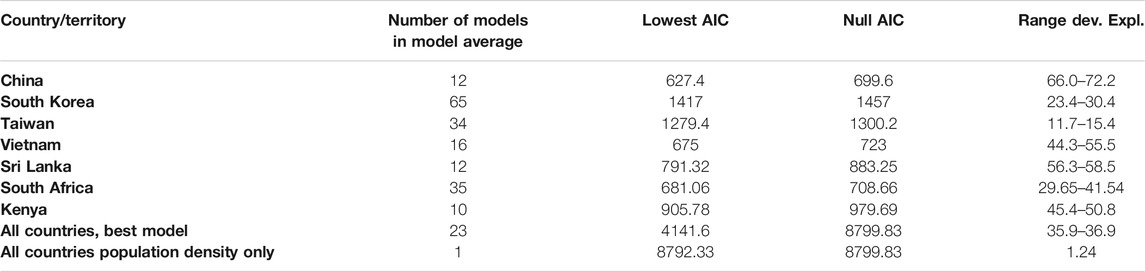
TABLE 3. Description of models used in the model averaging (all within 2 AIC values). Lowest AIC indicates the lowest AIC value for the models within each of the countries. Models in the model averaging are all within 2 AIC points of the lowest. Null AIC is the AIC of a regression with no covariates included. Note that the AIC values cannot be compared between countries, because they are using different data sets. AIC values can be compared between all countries, and all countries with population density only because they are using the same data set.

FIGURE 1

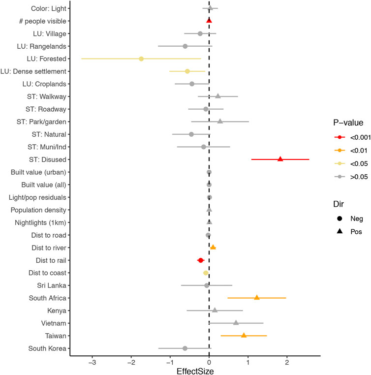
FIGURE 1. Effect size plots for all countries together. Color represents the p-value significance level, and the lines are the standard error for each term. Triangles denote a positive coefficient for a given factor, whereas circles denote a negative coefficient. The effect size is calculated as the median value of the factor times its coefficient.

FIGURE 2

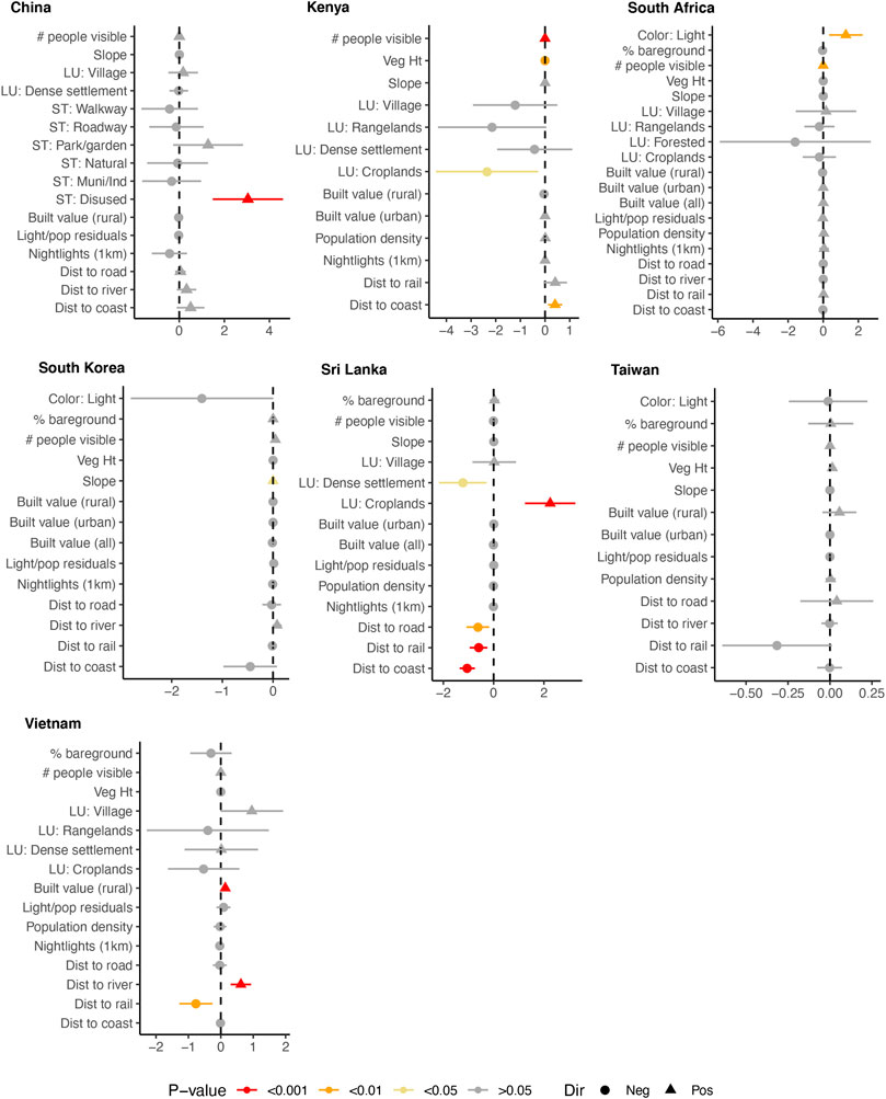
FIGURE 2. Effect size plots for China, Kenya, South Africa, South Korea, Sri Lanka, Taiwan, and Vietnam. Color represents the p-value significance level, and the lines are the standard error for each term. Triangles denote a positive coefficient for a given factor, whereas circles denote a negative coefficient. The effect size is calculated as the median value of the factor times its coefficient.

TABLE 4

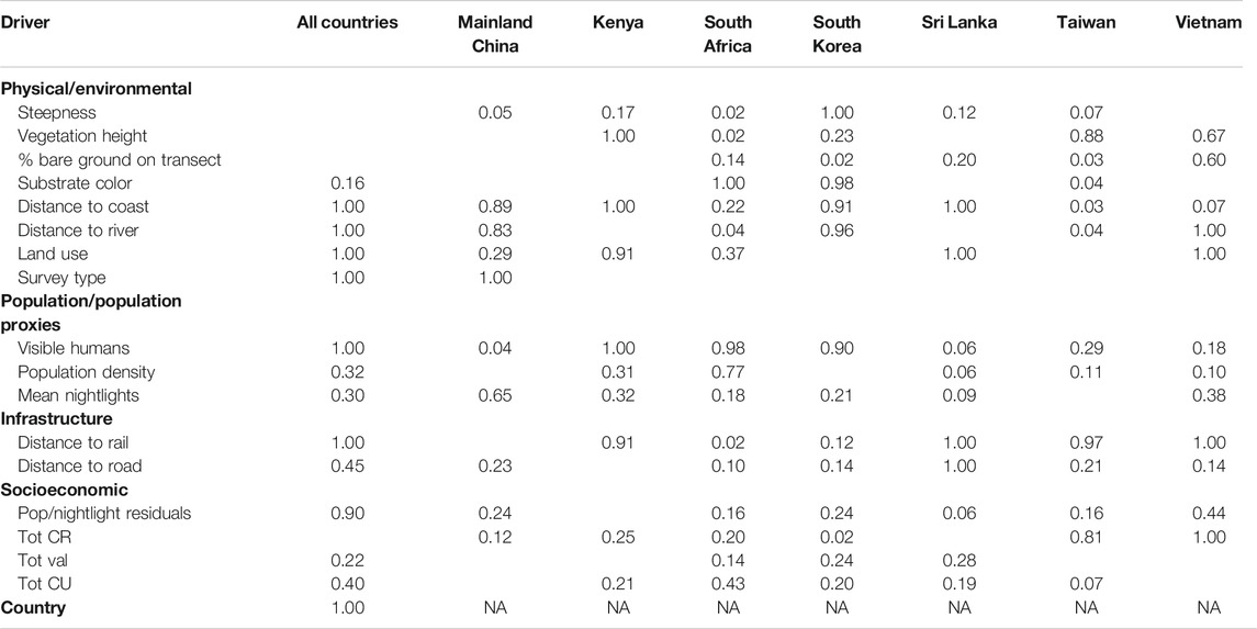
TABLE 4. Variable importance scores. Blank cells indicate that the driver was not present in the top models. Importance scores are calculated as the proportion of the models within the model averaging in which the driver appears.

How Similar (or Different) are the Drivers Between Countries?

For each country individually, we used the same analyses as above to identify the covariates that best described the variability in debris, with the same restrictions as above (Figure 2).

Do Models Based on Population Density Accurately Predict Debris?

To determine whether population density is an accurate proxy for debris, we ran a GAM using total debris counts as the response variable, and population density (within 1 km²) as the predictor variable. We compared the deviance explained and AIC with the null model, and with our full model (Table 3).

Results

The total number of items on each transect varied from 0–242 items. South Korea had the overall lowest average debris density (0.4 items/m²), while South Africa, had the highest (2.05 items/m²) based on inland surveys (Table 2).

What Drives the Distribution of Debris in Inland Areas?

For the combined models, significant terms included visible humans (positively correlated), landuse (forested and dense settlements lower than urban settlements), survey type (disused significantly greater than agriculture), distance to river (positively correlated), rail and coast (negatively correlated), and country (Figure 1). All of these terms appeared in all models, with a resulting effect size of 1.0 (Table 4). Population/nightlight residuals appeared in 90% of all models, while the other terms appeared in fewer than half of the models. It is worth nothing though, that either nightlights or population density did appear in 62% of the models.

How Similar (or Different) are the Drivers Between Countries?

Drivers were not completely consistent among countries. The best models for each country individually varied both in the terms included, as well as the directions of those terms (e.g., whether they were positively or negatively correlated with observed debris densities) (Figure 2; Table 4). Two terms appeared in all models: visible humans (positive correlation in all countries except Sri Lanka), and distance to the coast (negative correlation in all countries except mainland China and Kenya). A further six terms occurred in all but one country: slope (all but Vietnam), distance to the nearest rail (all but mainland China), light/population residuals (all but Kenya), total built value of the rural environment (all but Sri Lanka), mean nightlights (all but Taiwan) and distance to the nearest road (all but Kenya).

For individual country models, significant terms included visible humans (South Africa, Kenya), slope of land (South Korea), vegetation height (Kenya), substrate color (South Africa), distance to the coast (Sri Lanka, Kenya), distance to the nearest rail (Vietnam, Sri Lanka), distance to the nearest road (Sri Lanka), total built value (rural) (Vietnam), landuse (Sri Lanka, Kenya), and distance to the nearest river (Vietnam) (Figure 1).

Variable importance scores were similarly diverse, with different terms appearing more frequently in different countries (Table 4).

Do Models Based on Population Density Accurately Predict Debris?

The relationship between population density alone and total debris was significant and positive (p < 0.001). The deviance explained was 1.25%. The deviance explained of the 23 full models contributing to the model averaging was between 35.9–36.9.

Discussion

To date, most studies of plastic leakage rates consist either of surveys conducted predominately at coastal or beach locations in a single region or country (e.g., Hardesty et al., 2017a; Schöneich-Argent et al., 2019), or rely on globally available proxy data to model predicted debris on a global or regional scale, without incorporating empirical data (e.g., Jambeck et al., 2015; Lebreton and Andrady, 2019; Borrelle et al., 2020; Lau et al., 2020). Here we combine the two approaches, using survey data to test the utility of a variety of local and global proxy layers.

What Drives the Distribution of Debris in Inland Areas?

Studies of debris on the open ocean and along coastlines have found that physical factors such as currents, waves, wind and tides have an important effect on the distribution and accumulation of debris (Olivelli et al., 2020; Van Sebille et al., 2020), but the drivers of inland debris distribution are less well understood.

When the data were pooled, land use (a globally measured covariate) survey type (a locally determined covariate), and Country, explained a significant amount of the variability in the data. The significant influence of survey type was driven in large part by the elevated levels of litter found in disused areas. Both land use and survey type were also found to be significant in studies conducted in both the United States and Australia (Hardesty et al., 2017b; Hardesty et al., 2017c). Other factors that contributed to the patterns observed included distance to coast, distance to railroad station, and distance to river. However, their effect sizes were considerably lower than land use, survey type, and country.

Previous work has shown that socio-economic status is one of the most influential factors in predicting debris, with higher socio-economic indicators associated with reduced debris loads (Schuyler et al., 2018a). This is likely due to a combination of influences including income, education, infrastructure, access to social structures, and behavioral norms (Ajzen, 1991). For the combined seven country model, three socio-economic indicators appeared among the best models; light/population residuals, the built value (urban), and the built value (all) (Figure 1). While none were statistically significant, they all contributed to explaining the variability in the data (and were thus included in the best models). The values for all three indicators trended toward a negative relationship with debris density, indicating that as an area was higher in socio-economic status, the debris loads were lower/reduced. This finding reflects the negative correlation between GDP and per capita mismanaged waste that has been reported in other work (Lebreton and Andrady, 2019). While richer countries tend to generate more waste per capita, they also tend to have better waste management systems, which ultimately results in a lower proportion of mismanaged waste. Here we showed that the trend reported on a county-wide scale, also holds on a sub-national level.

How Similar (or Different) are the Drivers Between Countries?

Overall, the individual models were quite good at explaining the variability in the debris data, with deviance explained values of up to 72% (Table 3). These models generally incorporated factors measured at the site level, such as local land use, vegetation height, survey type, and substrate color.

We found high heterogeneity between countries, both in terms of the magnitude of debris, and the most relevant drivers for the patterns observed. In fact, in the combined model, country is one of the strongest predictors of the total amount of debris reported. The differences observed between the countries remained present even after accounting for the driving factors measured, and may be a result of other underlying factors including political/social differences, legislation, and geography. This reveals another challenge in predicting debris leakage rates on a global level. Each country demonstrated different baseline quantities of debris, with substantial variability observed among survey sites, both within and among countries. This demonstrates the importance of establishing baselines and monitoring programs on a local and regional scale, rather than relying solely on large-scale, global model-based predictions.

Do Models Based on Population Density Accurately Predict Debris?

One goal of both land and ocean-based debris research is to understand and quantify the distribution of debris, which can inform efforts to both prevent waste leaking and to remove litter than has already arrived in the environment. Because it is impossible to sample ubiquitously, researchers rely on globally available data sets to provide proxy measures for the amount of waste or leakage in a given area. Loss rates are often based on population density (e.g., Van Sebille et al., 2012), and, increasingly, the proportion of mismanaged waste (e.g., Lebreton and Andrady, 2019) though occasionally factors such as runoff and artificial barriers may be incorporated into estimates (e.g., Lebreton et al., 2017). These predictions assume that debris leakage rates are proportional to population density, though there is little empirical evidence to support this hypothesis. In the United States, research showed that while land-based debris did increase with population where population densities are low, this relationship did not hold at higher population densities (Ribic et al., 2010). Cities, even in less developed countries, can leverage economies of scale, and may have better systems for managing waste. Thus, the relationship between population and mismanaged waste is not necessarily linear.

In our modeling of empirical data from seven different countries, neither local population density nor one proxy for population (nightlights) were among the most critical factors to explain the variability in the data. Many of the top models did not include either term, and their effect was never significant, whether looking at individual countries or at all countries combined. Moreover, population density was negatively correlated with debris in two of the five individual models in which it appears, and nightlights were negatively correlated with debris density in four of the six countries. In our model regressing population density alone against the total amount of debris across all survey sites, while the relationship was significant and positive, the deviance explained was only 1.25% of the pattern observed.

The distribution of sampling sites in individual countries is quite wide ranging, both geographically as well across the suite of social and environmental factors, land use and human activities (e.g., incorporating urban and rural sites). If population density is not a critical factor at this scale, it is unlikely that the pattern will be reversed at international or continental scales.

The results of the this work indicate that it is critical to develop a more nuanced approach for estimating debris levels, if we are to develop accurate predictive models. Debris densities are extremely heterogeneous, and vary depending on a range of factors, including broad scale characteristics such as land use, finer scale details such as survey type, socio-economic patterns, existing infrastructure and environmental factors. The underlying drivers of debris distribution are complex, and difficult to capture accurately. What is clear, though, is that in all of the models, population density alone did not adequately explain the observed debris distribution. Relying on population density as a primary (or sole!) proxy, as has been done previously, will lead to an inaccurate characterization of debris distributions, and potentially to flawed policy responses based accordingly.

We ranked the seven countries surveyed based on empirical data collected by our teams according to the total debris load. We compared these counts to the per capita rank presented in Jambeck et al. (2015). Our ranking is based on the country coefficient in the model with all countries, and therefore considers population and the other debris drivers in the model. We found very little similarity in rank between our empirical estimates and those reported by Jambeck et al. (2015) (Table 5). This is likely due to a combination of factors. First, our analyses included local variables, as well as additional global scale variables that the Jambeck paper did not incorporate. Second, our analyses were based on empirical data. Finally, our surveys took place at a city or watershed scale rather than at a country level. The differences between the relative rankings only serves to highlight the importance of accurate models based on empirical data, so that limited resources for addressing the problems of litter and mismanaged waste can be most effectively deployed.

TABLE 5

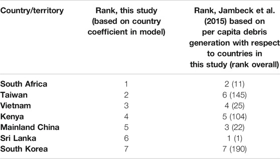
TABLE 5. Relative rankings of countries surveyed in this study as compared to relative rankings in Jambeck et al. (2015). Highest debris load = 1, lowest = 7.

Many studies that empirically quantify debris leakage are conducted along beaches and coastlines (Serra-Gonçalves et al., 2019). However, it is of critical importance to also measure inland debris if we are to fully understand loss rates to the environment. Debris from inland areas is transported to the sea via rivers, along roadways and by wind transport. Measuring debris in non-coastal areas helps to contextualize the factors that influence where debris originates in the environment, before it moves along various pathways, potentially arriving in the coastal or marine environment. Because of the high heterogeneity of inland areas, and the idiosyncratic nature of waste generation, it is crucial to design sampling that takes into account the inherent variability not only in the physical landscape, but also in the suite of factors that influence debris distribution.

Summary/Conclusion

Efforts to remove or prevent debris from entering the environment would be facilitated by a better understanding of the variability in its distribution, and the factors that affect debris density in the environment. The models presented here can also be used to derive large scale predictions of debris hotspots based not only on global data layers, but also on empirical data. These predictions could inform local and regional waste management policies and decisions on waste infrastructure. The results of this study demonstrate that the environmental context (e.g., landuse, site type) is critical in understanding and predicting the amount of debris in the environment. Importantly, population density is not the driving force behind debris distribution, and there is significant variability in the drivers of inland debris across countries. It is of critical importance to establish monitoring programs to understand the baseline levels of debris, not only in order to have accurate estimates of ocean debris inputs, but also so that the effectiveness of land-based interventions can be assessed.

Data Availability Statement

The raw data supporting the conclusions of this article will be made available by the authors, without undue reservation.

Author Contributions

QS, BH, and CW developed the methods. All authors contributed to data collection and logistics. QS and CW developed the analytical techniques. TL prepared GIS covariates. QS wrote the manuscript, with editing by BH, CW, RR, and JH.

Funding

This work has been funded by CSIRO Oceans and Atmosphere, Oak Family Foundation, Schmidt Marine Technology, the PM Angell Foundation and Earthwatch Institute Australia.

Conflict of Interest

The authors declare that the research was conducted in the absence of any commercial or financial relationships that could be construed as a potential conflict of interest.

Acknowledgments

We would like to extend our deepest gratitude to the tireless efforts of volunteers, students, and staff members who helped to collect data in the field. Also thank you to the two reviewers for their constructive comments.

References

Ajzen, I. (1991). The Theory of Planned Behavior. Organizational Behav. Hum. Decis. Process. 50, 179–211. doi:10.1016/0749-5978(91)90020-t

CrossRef Full Text | Google Scholar

Barnes, D. K. A., Galgani, F., Thompson, R. C., and Barlaz, M. (2009). Accumulation and Fragmentation of Plastic Debris in Global Environments. Phil. Trans. R. Soc. B 364, 1985–1998. doi:10.1098/rstb.2008.0205

PubMed Abstract | CrossRef Full Text | Google Scholar

Bartoń, K. (2018). MuMIn: Multi-Model Inference. R package version 1.42.1. https://CRAN.R-project.org/package=MuMIn.

Google Scholar

Battulga, B., Kawahigashi, M., and Oyuntsetseg, B. (2019). Distribution and Composition of Plastic Debris along the River Shore in the Selenga River Basin in Mongolia. Environ. Sci. Pollut. Res. 26, 14059–14072. doi:10.1007/s11356-019-04632-1

PubMed Abstract | CrossRef Full Text | Google Scholar

Beaumont, N. J., Aanesen, M., Austen, M. C., Börger, T., Clark, J. R., Cole, M., et al. (2019). Global Ecological, Social and Economic Impacts of Marine Plastic. Mar. Pollut. Bull. 142, 189–195. doi:10.1016/j.marpolbul.2019.03.022

PubMed Abstract | CrossRef Full Text | Google Scholar

Borrelle, S. B., Ringma, J., Law, K. L., Monnahan, C. C., Lebreton, L., Mcgivern, A., et al. (2020). Predicted Growth in Plastic Waste Exceeds Efforts to Mitigate Plastic Pollution. Science 369, 1515–1518. doi:10.1126/science.aba3656

PubMed Abstract | CrossRef Full Text | Google Scholar

Burnham, K. P., and Anderson, D. R. (2002). Model Selection and Multi-Model Inference: A Practical Information-Theoretic Approach. New York, NY: Springer-Verlag

Cordova, M. R., and Nurhati, I. S. (2019). Major Sources and Monthly Variations in the Release of Land-Derived Marine Debris from the Greater Jakarta Area, Indonesia. Scientific Rep. 9, 1–8. doi:10.1038/s41598-019-55065-2

PubMed Abstract | CrossRef Full Text | Google Scholar

Derraik, J. G. B. (2002). The Pollution of the Marine Environment by Plastic Debris: a Review. Mar. Pollut. Bull. 44, 842–852. doi:10.1016/s0025-326x(02)00220-5

PubMed Abstract | CrossRef Full Text | Google Scholar

Gall, S. C., and Thompson, R. C. (2015). The Impact of Debris on Marine Life. Mar. Pollut. Bull. 92, 170–179. doi:10.1016/j.marpolbul.2014.12.041

PubMed Abstract | CrossRef Full Text | Google Scholar

Geyer, R., Jambeck, J. R., and Law, K. L. (2017). Production, Use, and Fate of All Plastics Ever Made. Sci. Adv. 3, e1700782. doi:10.1126/sciadv.1700782

PubMed Abstract | CrossRef Full Text | Google Scholar

Hardesty, B. D., Lawson, T., Van Der Velde, T., Lansdell, M., and Wilcox, C. (2017a). Estimating Quantities and Sources of Marine Debris at a Continental Scale. Front. Ecol. Environ. 15, 18–25. doi:10.1002/fee.1447

CrossRef Full Text | Google Scholar

Hardesty, B. D., Schuyler, Q., Lawson, T. J., Opie, K., and Wilcox, C. (2016). Understanding Debris Sources and Transport from the Coastal Margin to the Ocean, in Final Report to the National Packaging Covenant Industry Association. (Hobart, TS: CSIRO)

Google Scholar

Hardesty, B. D., Schuyler, Q., Willis, K., Lawson, T. J., and Wilcox, C. (2017b). Policy and Practices Analysis to Reduce Debris Inputs to the Environment. A Final Report to the National Packaging Covenant Industry Association, in Final Report to the National Packaging Covenant Industry Association. (Hobart, TS: CSIRO)

Google Scholar

Hardesty, B. D., Wilcox, C., Schuyler, Q., Lawson, T. J., and Opie, K. (2017c). Developing a Baseline Estimate of Amounts, Types, Soures, and Distribution of Coastal Litter - an Analysis of US Marine Debris Data. Version 1.2. (Hobart, TS: CSIRO)

Jambeck, J. R., Geyer, R., Wilcox, C., Siegler, T. R., Perryman, M., Andrady, A., et al. (2015). Plastic Waste Inputs from Land into the Ocean. Science 347, 768–771. doi:10.1126/science.1260352

PubMed Abstract | CrossRef Full Text | Google Scholar

Kershaw, P., and Rochman, C. (2015). Sources, Fate and Effects of Microplastics in the Marine Environment: Part 2 of a Global Assessment. Reports and studies-IMO/FAO/Unesco-IOC/WMO/IAEA/UN/UNEP Joint Group of Experts on the Scientific Aspects of Marine Environmental Protection (GESAMP) eng no. 93.

Google Scholar

Lau, W. W. Y., Shiran, Y., Bailey, R. M., Cook, E., Stuchtey, M. R., Koskella, J., et al. (2020). Evaluating Scenarios toward Zero Plastic Pollution. Science 369, 1455–1461. doi:10.1126/science.aba9475

PubMed Abstract | CrossRef Full Text | Google Scholar

Lebreton, L., and Andrady, A. (2019). Future Scenarios of Global Plastic Waste Generation and Disposal. Palgrave Commun. 5, 1–11. doi:10.1057/s41599-018-0212-7

CrossRef Full Text | Google Scholar

Lebreton, L. C.-M., Greer, S. D., and Borrero, J. C. (2012). Numerical Modelling of Floating Debris in the World's Oceans. Mar. Pollut. Bull. 64, 653–661. doi:10.1016/j.marpolbul.2011.10.027

PubMed Abstract | CrossRef Full Text | Google Scholar

Lebreton, L. C. M., Van Der Zwet, J., Damsteeg, J.-W., Slat, B., Andrady, A., and Reisser, J. (2017). River Plastic Emissions to the World’s Oceans. Nat. Commun. 8, 15611. doi:10.1038/ncomms15611

PubMed Abstract | CrossRef Full Text | Google Scholar

Martins, I., Rodríguez, Y., and Pham, C. K. (2020). Trace Elements in Microplastics Stranded on Beaches of Remote Islands in the NE Atlantic. Mar. Pollut. Bull. 156, 111270. doi:10.1016/j.marpolbul.2020.111270

PubMed Abstract | CrossRef Full Text | Google Scholar

Miladinova, S., Macias, D., Stips, A., and Garcia-Gorriz, E. (2020). Identifying Distribution and Accumulation Patterns of Floating Marine Debris in the Black Sea. Mar. Pollut. Bull. 153, 110964. doi:10.1016/j.marpolbul.2020.110964

PubMed Abstract | CrossRef Full Text | Google Scholar

Napper, I. E., Davies, B. F. R., Clifford, H., Elvin, S., Koldewey, H. J., Mayewski, P. A., et al. (2020). Reaching New Heights in Plastic Pollution-Preliminary Findings of Microplastics on Mount Everest. One Earth 3, 621–630. doi:10.1016/j.oneear.2020.10.020

CrossRef Full Text | Google Scholar

Olivelli, A., Hardesty, D., and Wilcox, C. (2020). Coastal Margins and Backshores Represent a Major Sink for Marine Debris: Insights from a Continental-Scale Analysis. Environ. Res. Lett. 15. doi:10.1088/1748-9326/ab7836

CrossRef Full Text | Google Scholar

R Core Team (2018). R: A Language and Environment for Statistical Computing. Vienna, Austria: R foundation for statistical computing.

Ribic, C. A., Sheavly, S. B., Rugg, D. J., and Erdmann, E. S. (2010). Trends and Drivers of Marine Debris on the Atlantic Coast of the United States 1997-2007. Mar. Pollut. Bull. 60, 1231–1242. doi:10.1016/j.marpolbul.2010.03.021

PubMed Abstract | CrossRef Full Text | Google Scholar

Schöneich-Argent, R. I., Hillmann, F., Cordes, D., Wansing, R. A. D., Merder, J., Freund, J. A., et al. (2019). Wind, Waves, Tides, and Human Error? - Influences on Litter Abundance and Composition on German North Sea Coastlines: An Exploratory Analysis. Mar. Pollut. Bull. 146, 155–172. doi:10.1016/j.marpolbul.2019.05.062

PubMed Abstract | CrossRef Full Text | Google Scholar

Schuyler, Q., Hardesty, B. D., Lawson, T., Opie, K., and Wilcox, C. (2018a). Economic Incentives Reduce Plastic Inputs to the Ocean. Mar. Pol. 96, 250-255. doi:10.1016/j.marpol.2018.02.009

CrossRef Full Text | Google Scholar

Schuyler, Q., Willis, K., Mann, V., Wilcox, C., and Hardesty, B. D. (2018b). Handbook of Survey Methodology – Plastics Leakage. Australia: CSIRO.

Serra-Gonçalves, C., Lavers, J. L., and Bond, A. L. (2019). Global Review of Beach Debris Monitoring and Future Recommendations. Environ. Sci. Technol. 53, 12158–12167. doi:10.1021/acs.est.9b01424

PubMed Abstract | CrossRef Full Text | Google Scholar

UNISDR (2015). Making Development Sustainable: The Future of Disaster Risk Management. Global Assessment Report on Disaster Risk Reduction. Geneva, Switzerland: United Nations Office for Disaster Risk Reduction (UNISDR)

Van Calcar, C. J., and Van Emmerik, T. H. M. (2019). Abundance of Plastic Debris across European and Asian Rivers. Environ. Res. Lett. 14, 124051. doi:10.1088/1748-9326/ab5468

CrossRef Full Text | Google Scholar

Van Sebille, E. (2014). Adrift.org.au - A free, quick and easy tool to quantitatively study planktonic surface drift in the global ocean. J. Exp. Mar. Biol. Ecol. 461, 317–322. doi:10.1016/j.jembe.2014.09.002

CrossRef Full Text | Google Scholar

Van Sebille, E., Aliani, S., Law, K. L., Maximenko, N., Alsina, J. M., Bagaev, A., et al. (2020). The Physical Oceanography of the Transport of Floating Marine Debris. Environ. Res. Lett. 15–023003. doi:10.1088/1748-9326/ab6d7d

CrossRef Full Text | Google Scholar

Van Sebille, E., England, M. H., and Froyland, G. (2012). Origin, Dynamics and Evolution of Ocean Garbage Patches from Observed Surface Drifters. Environ. Res. Lett. 7, 044040. doi:10.1088/1748-9326/7/4/044040

CrossRef Full Text | Google Scholar

Van Sebille, E., Wilcox, C., Lebreton, L., Maximenko, N., Hardesty, B. D., Van Franeker, J. A., et al. (2015). A Global Inventory of Small Floating Plastic Debris. Environ. Res. Lett. 10, 124006. doi:10.1088/1748-9326/10/12/124006

CrossRef Full Text | Google Scholar

Vidyasakar, A., Krishnakumar, S., Kasilingam, K., Neelavannan, K., Bharathi, V. A., Godson, P. S., et al. (2020). Characterization and Distribution of Microplastics and Plastic Debris along Silver Beach, Southern India. Mar. Pollut. Bull. 158, 111421. doi:10.1016/j.marpolbul.2020.111421

PubMed Abstract | CrossRef Full Text | Google Scholar

Wessel, C., Swanson, K., Weatherall, T., and Cebrian, J. (2019). Accumulation and Distribution of Marine Debris on Barrier Islands across the Northern Gulf of Mexico. Mar. Pollut. Bull. 139, 14–22. doi:10.1016/j.marpolbul.2018.12.023

PubMed Abstract | CrossRef Full Text | Google Scholar

Wood, S. N. (2011). Fast Stable Restricted Maximum Likelihood and Marginal Likelihood Estimation of Semiparametric Generalized Linear Models. J. R. Stat. Scoieety (B) 73, 3–36. doi:10.1111/j.1467-9868.2010.00749.x

CrossRef Full Text | Google Scholar