Potential for High Fidelity Global Mapping of Common Inland Water Quality Products at High Spatial and Temporal Resolutions Based on a Synthetic Data and Machine Learning Approach

Introduction

Widespread increase of lake phytoplankton blooms is causing global eutrophication to intensify (Ho et al., 2019). The substantial increase in eutrophication will potentially increase methane emissions from these systems by 30–90% over the next century, substantially contributing to global warming (Beaulieu et al., 2019). Recent advancements in sensor technology and algorithm development have allowed for improved measurements of coastal and inland waters (Hu, 2009; Matthews et al., 2012; Palmer et al., 2015b; Smith et al., 2018; Pahlevan et al., 2020). Given the increased attention placed on retrieving eutrophication metrics for inland water bodies, numerous studies have attempted radiometric retrieval of chlorophyll-a (chl-a) or phycocyanin (PC), the diagnostic pigment within cyanobacteria, with varying degrees of success (see reviews by Ogashawara, 2020; Odermatt et al., 2012; Blondeau-Patissier et al., 2014; Matthews, 2011; Gholizadeh et al., 2016). Retrieval of chl-a concentration has been significantly developed, and is generally more robust for trophic delineation; however, PC is highly specific to cyanobacteria and is thus a better indicator of potential water toxicity (Stumpf et al., 2016). Given the fine-scale horizontal and vertical heterogeneity of productive waters (Kutser, 2004; Kutser et al., 2008; Kravitz et al., 2020) and lack of standardization of field methods, laboratory procedures, and analysis for mixed freshwater phytoplankton assemblages, it is difficult to conduct high impact optical sensitivity studies. Consequently, trustworthy in-situ data for productive coastal and inland waters is limited compared to combined global datasets for ocean calibration and validation, which critically hinders our capacity to execute global baseline studies, as well as to identify global trends using archival imagery. It is therefore imperative that we develop suitable algorithms for optical constituent retrieval for current and planned missions, with a full understanding of the associated uncertainties and limitations.

Machine learning (ML) and deep learning (DL) approaches are quickly becoming recognized as state-of-the-art for classification and regression type problems, and remote sensing is ideally suited to such approaches (Ma et al., 2019, and references therein). The majority of ML and DL development and application have been within the terrestrial remote sensing community (Ball et al., 2017; Li et al., 2018; Maxwell et al., 2018; Ghorbanzadeh et al., 2019), although recent research reveals the benefit of ML and DL approaches for aquatic purposes (Pahlevan et al., 2020; Balasubramanian et al., 2020; Watanabe et al., 2020; Sagan et al., 2020; Peterson et al., 2020; Hafeez et al., 2019; Ruescas et al., 2018). While these studies generally found better performance of ML and DL approaches over traditional empirical or semi-analytical methods, most note that the advanced models were trained on too few datapoints, and would greatly benefit from expanded datasets. DL architectures in particular substantially benefit from greater volumes of high-quality training data. Vastly more coincident reflectance—biophysical parameter pairs, PC in particular, are required to train new and improved multi-parameter inversions for synoptic image analysis at global scales.

Radiative transfer modeling (RTM) has proven instrumental to furthering our understanding of coastal aquatic optical relationships in the form of numerous parameterized case studies (Dall’Olmo and Gitelson, 2005; Dall’Olmo and Gitelson, 2006; Gilerson et al., 2007; Gilerson et al., 2008; Lain et al., 2014; Lain et al., 2016; Evers-King et al., 2014). Few, however, have expanded these analyses to cyanobacteria dominated inland waters (Kutser, 2004; Metsamma et al., 2006; Matthews and Bernard, 2013; Kutser et al., 2006). RTM has proved advantageous for the development of large synthetic datasets to address the scarcity of valid in-situ data available to train neural network (NN) retrieval models (Doerffer and Schiller, 2008; Arabi et al., 2016; Brockmann et al., 2016; Fan et al., 2017; Hieronymi et al., 2017). While a few of these algorithms such as the Case 2 Extreme OLCI Neural Network Swarm (ONNS, Hieronymi et al., 2017) and Case 2 Regional Coast Color (C2RCC, Brockmann et al., 2016) include samples for extremely absorbing and scattering cases due to global instances of elevated colored dissolved organic matter (CDOM) and non-algal particles (NAP), the phytoplankton component of these models is not optimized for adequate pigment retrieval in optically complex eutrophic inland water (Palmer et al., 2015a; Kutser et al., 2018; Kravitz et al., 2020).

The fundamental building blocks of aquatic RTM rely on accurate parameterization of the inherent optical properties (IOPs; i.e., absorption and scattering properties) of all light altering constituents in a volume of water. Fan et al. (2017) and C2RCC utilize chlorophyll-specific phytoplankton absorption (${\text{a}}_{\text{phy}}^{\text{*}}$) measurements directly from the NASA bio-Optical Marine Algorithm Dataset (NOMAD), while ONNS uses five ${\text{a}}_{\text{phy}}^{\text{*}}$ shapes derived from cluster and derivative analysis of various phytoplankton cultures (Xi et al., 2015). These studies rely heavily on phytoplankton absorption characteristics as the main driver for resulting functional type and biomass related differences in modeled reflectances. Such an assumption is generally adequate for oligotrophic to mesotrophic water conditions, whereas the absence of a wavelength dependent, phytoplankton-specific backscattering term, or the use of backscattering relating only to gross particulate, is too simplistic for eutrophic conditions and generally underperforms in more productive waters (Lain et al., 2014; Lain et al., 2016). The scattering phase function, critical for fully realizing the underwater light field, is generally approximated as a simple functional form for mathematical simplicity (Mobley et al., 2002) or derived from Mie theory, which over-generalizes phytoplankton particles as spherical homogenous structures. Indeed, some studies that characterized the backscattering properties of various monospecific cultures have found a prominent deviation from the homogenous sphere model, which yields a poor simplification of the complex cellular structures found in bloom-forming phytoplankton (Quirantes and Bernard, 2004; Vaillancourt et al., 2004; Whitmire et al., 2007; Zhou et al., 2012; Matthews and Bernard, 2013). This is particularly important for productive inland waters where blooms of potentially toxic cyanobacteria are becoming more prevalent. Cyanobacteria, Mycrocystis aeruginosa especially, appear to be extremely efficient backscatterers (Zhou et al., 2012), which has been attributed to their internal gas vacuoles (Matthews and Bernard, 2013). Due to strong effects of gas vacuoles on attenuation, rather than absorption, drastic differences in water-leaving reflectance occur in mixed cyanobacteria assemblages. Thus, vacuolate induced spectral scattering (Ganf et al., 1989; Walsby et al., 1995) cannot be overlooked when parameterizing RTMs for inland water application. To address these over-simplifications, the Equivalent Algal Populations (EAP) model provides an alternative assemblage-based particle modeling approach, simulating phytoplankton IOPs derived from differences in cell and assemblage size distributions, dominant pigmentation, cell composition, and ultrastructure (Bernard et al., 2009; Lain et al., 2014).

While Pahlevan et al. (2020) and Balasubramanian et al. (2020) present highly convincing results for the transition to ML based models for aquatic particle retrievals using multi-spectral sensors, the authors note that adequate atmospheric correction (AC) of top of atmosphere (TOA) radiances to bottom of atmosphere (BOA) reflectances remains one of the largest hurdles to robust, operational space-based water quality retrievals. Baseline type algorithms, which have proven to be robust estimators of trophic status, and relatively insensitive to poor AC, have been utilized on partially corrected bottom-of-Rayleigh reflectance (BRR) in an attempt to bypass the requirement for a full AC (Binding et al., 2011; Matthews et al., 2012; Palmer et al., 2015c). This approach is indeed helpful for smaller water bodies where AC-induced uncertainty remains very high (Kravitz et al., 2020). Thus, it follows that ML type models should also perform adequately when utilized on TOA data for inland water pixels. However, relatively few studies have quantified the actual fraction of the isolated water-leaving signal that reaches the satellite sensor over productive inland water bodies. Utilizing TOA data is theoretically more feasible for turbid waters due to the elevated water signal from increased particulate backscattering compared to “darker” oligotrophic waters, which are dominated by water absorption. It is quite often cited that of the total radiance signal reaching a satellite over water, roughly 10% is due to the upwelling water-leaving radiance (L_w), with atmospheric aerosols and molecular (Rayleigh) scattering contributing the majority of the signal. However, in a localized modeling study, Martins et al. (2017) found that L_w had the potential to reach ∼43% of the total signal for red-edge bands of Sentinel-2 MSI over turbid lakes in the Amazon. It is important to understand the extent of the water signal at TOA and its sensitivity to certain water and atmospheric parameters in order to more thoroughly evaluate models that use TOA data.

Here, we aim to explore the potential for developing quick, robust multi-parameter aquatic retrieval models for both multi-spectral and hyper-spectral sensor specifications using a combined synthetic data and ML approach for productive inland waters. Our goal is to begin to simulate the immense natural optical variability of inland waters and to address the issues described above. Novel aspects of the synthetic dataset presented here include: 1) physics-based, two-layered, size and type specific phytoplankton IOPs for mixed eukaryotic/cyanobacteria assemblages, 2) calculations of mixed assemblage chl-a fluorescence, 3) modeled PC concentration, 4) and paired sensor-specific TOA reflectances, which include optically extreme cases and contribution of green vegetation adjacency. Below, we first describe the parameterization of RTM, followed by an examination of typical survived L_w signal at TOA, a description and assessment of state-of-the-art ML retrieval models, and application to multi-spectral imagery with a semi-quantitative validation against in-situ data.

Parameterization of Radiative Transfer Model

Aquatic RTM

For consistency with natural optical relationships, the IOPs of four datasets were compiled based on the domination of a particular optical constituent. The EcoLight RTM was then used to derive water-leaving reflectances from the IOP builds. The first dataset is modeled as typical Case 1 waters where water and phytoplankton provide the bulk of the optical signal and represent oligotrophic conditions. The bio-optical model in this dataset closely follows that of Lee (2003), wherein other optical constituents co-vary with phytoplankton biomass. The other three datasets resemble cyanobacteria dominated inland waters, CDOM dominated waters, and inorganic sediment dominated waters where more complex optical relationships persist and optical constituents do not tend to co-vary (Brewin et al., 2017). A four-component bio-optical model was used to generate the IOPs of these hypothetical inland water cases to be used in the EcoLight RTM (Lee, 2006; Gilerson et al., 2007):

$a\left(\lambda \right)=a_w\left(\lambda \right)+a_g\left(\lambda \right)+a_{phy}\left(\lambda \right)+a_{nap}\left(\lambda \right)(1)$

where $a_w\left(\lambda \right), a_g\left(\lambda \right), a_{phy}\left(\lambda \right),$ and $a_{nap}\left(\lambda \right)$ represent the spectral absorptions of water, a combined CDOM/detritus term, phytoplankton, and non-algal particles (NAP), respectively (refer to Supplementary Appendix A, Table A1, for a full list of definitions of symbols and units used throughout this manuscript). Except for the Case 1 dataset, which is defined solely on chlorophyll-a concentration (C_chl) and relationships governing the co-variation of other constituents with C_chl, the three other datasets are defined by independent values of C_chl, the concentration of nonalgal particles (C_nap), and the absorption of CDOM at 440 nm (a_g(440)). Great care was taken to ensure that constituent ranges were appropriate and based on natural populations from the LIMNADES in-situ inland water dataset (Spyrakos et al., 2018). A table of mode values and standard deviations used for the lognormal distributions within each dataset can be found in Supplementary Appendix A, Table A3. To generate synthetic datasets representative of natural waters, values of all constituents were randomly selected from the described lognormal distributions. Derivation and equations used in modeling components other than phytoplankton are common to studies that have parameterized models for Case 2 waters (Bukata, 1995; Twardowski et al., 2001; Gilerson et al., 2007) and can also be found in Supplementary Appendix A, Table A2.

Phytoplankton Component

The total spectral phytoplankton component in Eq. 1 is modeled as a product of C_chl and the specific chlorophyll absorption spectrum.

$a_{phy}\left(\lambda \right)=C_{chl}\ast a_{chl}^{\ast }\left(\lambda \right)(2)$

where $a_{chl}^{\ast }\left(\lambda \right)$ is the spectral specific chlorophyll absorption spectrum in m²/mg. Phytoplankton specific IOPs (SIOPs) for this work are based on the physics-based two-layered spherical Equivalent Algal Population (EAP) model, where population-specific refractive indices are used to derive IOPs (Bernard et al., 2009; Lain and Bernard, 2018). The two-layered spherical geometry consists of a core sphere, acting as the cytoplasm, and a shell sphere acting as the chloroplast. The EAP model calculates, from first principles, biophysically-linked phytoplankton absorption and scattering characteristics from particle refractive indices reflecting the primary light-harvesting pigments of various phytoplankton groups (Lain et al., 2014; Lain and Bernard, 2018). IOPs are calculated at 5 nm spectral resolution between 200 and 900 nm and integrated over an entire equivalent size distribution represented by effective diameters (D_eff) between 1 and 50 μm (Bernard et al., 2007; Lain et al., 2016). For a hypothetical eukaryotic population, refractive indices are derived from blooms in the Benguela upwelling off southern Africa, which is typically dominated by chlorophyll-a (chl-a) and the carotenoid pigments, fucoxanthin and peridinin, which are the main light harvesting pigments in diatoms and dinoflagellates, respectively. Because there are minimal differences within carotenoid pigment refractive indices and absorption, these two groups were combined into a generalized set of chl-a—carotenoid IOPs (Bernard et al., 2009; Organelli et al., 2017). The EAP model has been consistently validated and is considered an accurate phytoplankton model for coastal and inland waters (Evers-King et al., 2014; Mathews and Bernard, 2013; Lain et al., 2016; Smith et al., 2018).

The EAP two-layered sphere model has also been used to derive IOPs for the optically complex cyanobacteria M. aeruginosa (Matthews and Bernard, 2013). In this instance, the core layer is assigned to a highly scattering vacuole, while the shell layer acts as the chromatoplasm. M. aeruginosa is modeled with a D_eff of 5 μm for consistency with natural populations. For derivation of the complex refractive indices, influence of gas vacuolation, and tuning of the two-layered model for cyanobacteria, see Matthews and Bernard (2013). IOPs for the cyanobacteria Aphanizomenon, Anabaena cirinalis and non-vacuolate Nodularia spumigena, which were measured in the laboratory, are also included in the dataset (Kutser et al., 2006). The final phytoplankton SIOPs used in the RTM can be found in Supplementary Appendix A, Figure A1.

To account for optical variation due to mixed populations, the $a_{chl}^{\ast }\left(\lambda \right)$ term in Eq. 2 is modeled as an admixture of eukaryotic and cyanobacteria SIOPs based on a series of weighting factors. Total $a_{chl}^{\ast }\left(\lambda \right)$ is therefore calculated as the sum of the cyanobacteria and eukaryotic populations:

$a_{chl}^{\ast }\left(\lambda \right)=S_f\left(a_{cy}^{\ast }\left(\lambda \right)\right)+(1-S_f)\left(a_{euk}^{\ast }\left(\lambda \right)\right)(3)$

where S_f = [0.1,0.2,0.3,0.4,0.5,0.6,0.7,0.8,0.9,1.0], ${\text{a}}_{\text{cy}}^{\text{*}}$ is the chlorophyll-specific absorption of the cyanobacteria population and ${\text{a}}_{\text{euk}}^{\text{*}}$ is the chlorophyll-specific absorption for the carotenoid containing eukaryotic population. Total scattering and backscattering coefficients of the phytoplankton component ($b_{phy}\left(\lambda \right)\text{and}{b}_{bphy}\left(\lambda \right), \text{respectively}$) are calculated in a similar manner using EAP derived spectral chlorophyll-specific scattering and backscattering terms (Supplementary Appendix A).

The admixture weighting factor and input D_eff for the eukaryotic population were also randomly varied for the RTM, albeit with some constraints. Several studies have shown that for natural populations of oligotrophic to mesotrophic waters, ${\text{a}}_{\text{euk}}^{\text{*}}$ tends to decrease with increasing C_chl (Bricaud et al., 1995; Babin et al., 1996). This rule is not as strict in more complex inland and coastal waters, but rough relationships have been observed (Matthews and Bernard, 2013). Due to the nature of the EAP model, the magnitudes of the resulting SIOPs are highly dependent on the particle size. To generalize this natural relationship in our RTM, input phytoplankton SIOPs of the carotenoid containing population were constrained by D_eff as: 5 < D_eff < 20 μm for 0 < C_chl < 20 mg/m³, 15 < D_eff < 35 μm for 20 < C_chl < 50 mg/m³, and 30 < D_eff < 45 μm for C_chl > 50 mg/m³.

Ranges for appropriate cyanobacteria admixture weighting must also be comparable to natural variations as a function of phytoplankton biomass. Randomization of weighting factors was constrained based on in-situ phytoplankton abundance and biomass collected from South African inland waters between 2016 and 2018 (Kravitz et al., 2020). For a comparison of the fraction of cyanobacteria abundance as a function of chl-a concentration for both field data and ranges used in the RTM, see Supplementary Figure S1. Given the field data, it was assumed that if cyanobacteria are part of the phytoplankton population, they will tend to dominate at higher biomass (i.e., it is rare to find low fractions of cyanobacteria as C_chl rises to extremely hypertrophic levels, if cyanobacteria are present). M. aeruginosa is known to produce extremely high biomass blooms, with the potential to form floating scum mats that can reach C_chl upwards of 20,000 mg/m³ (Matthews and Bernard, 2013). Extremely hypertrophic cases are reflected in the RTM. For C_chl greater than 500 mg/m³, only M. aeruginosa is included as there are no data showing blooms of such an extent for other species.

Chl-a Fluorescence

Chl-a fluorescence is potentially an important source of information regarding phytoplankton physiology, size, and/or identification (Greene et al., 1992; Behrenfeld et al., 2009), although to what extent remains uncertain. While an integral component of phytoplankton physiology, fluorescence is often omitted from RTMs [as in the case of Hieronymi et al. (2017) and Fan et al. (2017)] or is modeled as a simplistic Gaussian term centered at 685 nm with a full width half max (FWHM) of 25 nm (Gilerson et al., 2007; Huot et al., 2007). The magnitude of the depth-integrated radiance contribution by chl-a fluorescence at 685 nm has traditionally been calculated as in Eq. 4 (Huot et al., 2005; Huot et al., 2007; refer to Supplementary Appendix A for definitions of symbols and units).

$L_f\left(685\right)=0.54L_f^{-}\left(685\right)=0.54\frac{1{\varnothing }_f}{4\pi C_f}{Q}_a^{\ast }\left[Chl\right]\underset{400}{\overset{700}{{\displaystyle \int }}} \frac{a_{chl}^{\ast }\left(\lambda \right)E_o^{-}\left(\lambda \right)}{K\left(\lambda \right)+K_{Lu}\left(685\right)}\text{d}\lambda (4)$

This modeling approach is an oversimplification for natural coastal and cyanobacteria dominated waters. The approach above assumes a purely eukaryotic, photosynthetic carotenoid-containing phytoplankton assemblage. In other words, it assumes that the modeled population contains all intracellular chl-a in the fluorescing photosystem II (PSII). Emission spectra of chl-a are a response to photosynthetic pigments that harvest light in PSII. However, cyanobacteria generally contain only 10–20% of their total cellular chl-a in PSII, with no accessory chlorophylls or carotenoids, and with the remaining cellular chl-a located in non-fluorescing photosystem I (PSI) (Johnsen and Sakshaug, 2007; Simis et al., 2012). A second oversimplification pertains to the shape of the modeled Gaussian fluorescence emission. In reality, while chl-a fluorescence does indeed have a major fluorescence emission around 685 nm, it also has an adjacent vibrational satellite emission centered around 730–740 nm (Govindjee, 2004 and references therein; Lu et al., 2016). Although generally smaller in amplitude due to increased absorption from water farther into the near-infrared (NIR), this 730–740 nm fluorescence emission can potentially contribute to the water leaving radiance. Supplementary Appendix B.1 details an updated mathematical derivation for the shape and magnitude of the chl-a fluorescence signal associated with mixed algal populations, which takes into account differences in PSII physiology for cyanobacteria and eukaryotic populations. Equations B1, B2, and B3 were applied to every synthetic spectra to calculate, and add, the modeled chl-a fluorescence spectrum.

Phycocyanin Concentration

While the EcoLight radiative transfer code allows C_chl to be defined as an input to the model, C_pc must be modeled independently. The calculation of C_pc can be accomplished as follows (Simis et al., 2005):

$\text{Cpc }=a_{pc}\left(\text{620}\right)\text{/}{a}_{pc}^{\ast }\left(\text{620}\right)(5)$

where $a_{pc}$(620) is the total absorption due to PC at 620 nm and $a_{pc}^{\ast }$(620) is the specific absorption coefficient of PC at 620 nm. The $a_{pc}$(620) term must be corrected for the absorption of all other optical constituents and pigments at 620 nm. Most existing methods only correct for absorption at 620 nm due to chl-a and not due other accessory pigments; thus, studies suggest that at low PC concentrations (<50 mg/m³), estimated $a_{pc}$(620) is not fully corrected for other pigment or constituent absorptions, resulting in overestimated C_pc (Simis et al., 2007; Yacobi et al., 2015). The mathematical logic for removal of the absorption due to chl-a and its accessory pigments, chl-b and chl-c, is further detailed in Supplementary Appendix B.2.

While the source of variability of $a_{pc}^{\ast }$(620) in nature is still not entirely clear, we can assume that first order variation can result from variable algal/cyanobacteria composition and biomass effects. Thus, varying $a_{pc}^{\ast }$(620) based on cyanobacteria dominance according to the admixture for each sample is a reasonable approach. Previous studies have generally relied on a fixed $a_{pc}^{\ast }$(620) value for PC estimation models. Considering that $a_{pc}^{\ast }$(620) has the potential to vary by a factor of 60 in nature (see Table 4 in Yacobi et al., 2015), holding it constant is a major oversimplification, especially for lower C_pc or for cases when cyanobacteria is not the dominant species. In particular, using an invariant $a_{pc}^{\ast }$(620) can result in a dramatic increase in error of PC retrieval when PC:chl-a < 0.5 (Simis et al., 2005; Randolph et al., 2008; Hunter et al., 2010; Li et al., 2015; Yacobi et al., 2015) or when C_pc < 50 mg/m³ (Simis et al., 2005; Ruiz-Verdu et al., 2008; Yacobi et al., 2015). By employing a model that allows $a_{pc}^{\ast }$(620) to vary based on cyanobacteria dominance, more appropriate values of $a_{pc}^{\ast }$(620) can be applied to situations of lower PC concentration. Given the consensus that a PC:chl-a ratio ≥0.5 (mg/m³) implies a cyanobacteria dominant water target (Simis et al., 2005; Hunter et al., 2010; Yacobi et al., 2015), our admixture of 0–1 was scaled to a PC:chl-a between 0 and 4, where an admixture of 0.6 (60% dominance by cyanobacteria in population) is equal to a PC:chl-a of 0.5. A strong non-linear relationship was found between PC:chla-a and $a_{pc}^{\ast }$(620) using in-situ data (Figures 1A,B), and is used in conjunction with each sample’s scaled admixture parameter to define a sample specific $a_{pc}^{\ast }$(620) as:

$a_{pc}^{\ast }\left(\text{620}\right)=0.0093{\left(S_{ad}\right)}^{-0.717}(6)$

where S_ad is the scaled admixture parameter. Once both $a_{pc}$(620) and $a_{pc}^{\ast }$(620) are known, Eq. 5 can be used to calculate a final PC concentration.

FIGURE 1

FIGURE 1. (A)$a_{pc}^{\ast }$(620) plotted as a function of PC:chl-a from Matthews and Bernard (2013) and Simis et al. (2005), denoted as M13 and S05, with best fit line in black, (B) Visual of admixture scaling, where an admixture of 0.6 (60% dominance by cyanobacteria in population) is equal to a PC:chl-a of 0.5, (C)$a_{pc}^{\ast }$(620) for four cyanobacteria groups plotted as a function of PC:chl-a for modeled synthetic data, (D)$a_{pc}^{\ast }$(620) plotted as a function of PC concentration, (E) PC plotted as function of chl-a concentration.

Modeled values for $a_{pc}^{\ast }$(620) using this methodology resulted in a mean and median $a_{pc}^{\ast }$(620) of 0.013 ± 0.017 and 0.0041, respectively. Simis et al. (2005) used an average value of 0.0095 m² (mg PC)⁻¹ calculated from their in-situ data while Matthews and Bernard (2013) found the mean $a_{pc}^{\ast }$(620) of various inland water bodies to range between 0.0072 and 0.0122. Yacobi et al. (2015) found that with C_pc > 10 mg/m³, $a_{pc}^{\ast }$(620) tended to converge on 0.007 m² (mg PC)⁻¹, but noted that this value is potentially too high. Other studies suggest $a_{pc}^{\ast }$(620) values between 0.004 and 0.005 m² (mg PC)⁻¹ (Li et al., 2015; Mishra et al., 2013; Simis and Kauko, 2012; Jupp et al., 1994). These values are more similar to our modeled absorption ranges, indicating that our calculated $a_{pc}^{\ast }$(620) are reasonable (Figure 1). At modeled PC concentrations >50 mg/m³, mean and median $a_{pc}^{\ast }$(620) stabilized at 0.0042 ± 0.002 and 0.0034, respectively. The majority of variability in modeled $a_{pc}^{\ast }$(620) occurred at a PC:chl-a < 0.5 or a C_pc < 50 mg/m³, consistent with previous findings (Mishra et al., 2013; Yacobi et al., 2015). The resulting PC:chl-a of the modeled synthetic data ranged between 0 and 4 mg/m³.

Atmospheric RTM Parameterization

The MODTRAN 5.0 radiative transfer software was used to propagate both L_w and R_rs from the aquatic modeling to OLCI at-sensor radiances. The radiance received by an optical sensor can be defined in simple terms following Bulgarelli et al. (2014) as:

$L_{tot}= L_{path}+L_{BG}+ t{L}_u(7)$

where $L_{tot}$ is the total radiance received by the sensor, $L_{path}$ is the path radiance, which defines the photons scattered into the instantaneous field of view (FOV) by the atmosphere alone, $L_{BG}$ is the background radiance from neighboring pixels, which are diffusely scattered into the sensor FOV, $L_u$ is the combined sky reflected and water leaving radiance at the sensor, and $t$ is the diffuse transmittance. $L_{BG}$ is considered as the radiance introduced due to the adjacency effect (AE), which can lead to large errors in derived products if inter-pixel non-uniformity is very large as in the case for neighboring vegetation, sand, or snow (Bulgarelli et al., 2017). Optical properties for a hypothetical atmospheric column for defining the RTM were compiled from level-2 (L2) derived products from the global Aerosol Robotic Network (AERONET) database (https://aeronet.gsfc.nasa.gov/). The parameters that were directly varied for the RTM included aerosol optical thickness at 550 nm (AOT550), the angstrom extinction coefficient (Ext), single scattering albedo (SSA), the altitude of the hypothetical water target (Alt), water vapor (H₂O), and percent adjacency of green grass vegetation (Adj). A tropospheric canned model was used to define the initial Mie-generated phase functions and asymmetry parameter, while Ext, SSA, and AOT550 were used to tweak the model based on randomly selected values from the L2 AERONET database. The ranges for these parameters are evident in Supplementary Figure S3. For each aquatic R_rs measurement, two random atmospheres were modeled, and for each atmosphere, a second identical run was performed with a random contribution of green grass adjacency between 0.5 and 50%, totaling four atmospheric radiative transfer runs per R_rs measurement. Spectral radiance reaching the satellite sensor was calculated as follows:

1. The weighted mean of mixed spectral albedo curves was computed based on the Adj parameter.

2. The atmospheric model was compiled in MODTRAN by tweaking the standard tropospheric canned model using randomly selected parameters (AOT550, SSA, H₂O, Ext, Alt, Adj).

3. L_u and L_w from Ecolight output were multiplied by atmospheric path transmittance ($t$) from MODTRAN output to obtain L_u and L_w at TOA (L_uTOA and L_wTOA, respectively).

4. Total radiance at TOA (L_totTOA) was calculated by adding L_uTOA to the MODTRAN derived atmospheric L_path, which is the radiance contribution from a scattering atmosphere.

5. All computations up to this point were performed at full MODTRAN 5 spectral resolution. The sensor specific spectral response functions (SRFs) were then applied to compute channel radiances.

6. Fraction of surviving L_w reaching the satellite sensor was calculated as L_wTOA/L_totTOA.

Radiance at TOA was converted to reflectance using an analytical derivation as in Hu et al. (2004):

${\rho }_t=\pi L_t^{\ast }/\left(F_{0}cos{\theta }_0\right)(8)$

where ${\rho }_t$ is sensor reflectance at TOA, $L_t^{\ast }$ is the calibrated at-sensor radiance after adjustment for ozone and gaseous absorption, F₀ is the extraterrestrial solar irradiance, and ${\theta }_0$ is the solar zenith angle. Adjustment for ozone and molecular species profiles are inherent to the MODTRAN RTM based on the specified atmospheric model used (Tropical, Mid-Latitude Summer, or Mid-Latitude Winter).

Data Preparation and Training

Data Smoothing and Clustering

Roughly 70,000 R_rs spectra were modeled with coincident C_chl, C_pc, C_nap, and associated IOPs. A clustering procedure was undertaken to identify distinct optical clusters with respect to reflectance within the dataset. Clustering of water types on the basis of optical properties has been commonly employed since the 1970s as a method to direct the application of Earth observation (EO) for aquatic purposes (Moore et al., 2001; Moore et al., 2009; Moore et al., 2014; Vantrepotte et al., 2012; Spyrakos et al., 2018). Clustering of optical data has historically been beneficial for demonstrating underlying bio-optical relationships and variability, and guiding the development and application of retrieval models. For consistency with previous clustering applications in coastal and inland waters, the functional data analysis (FDA) approach of Spyrakos et al. (2018) was closely followed, although only briefly discussed here. A full analysis of historical clustering techniques is beyond the scope of this paper, and readers are directed to Spyrakos et al. (2018 and references therein) for a more comprehensive overview of clustering approaches. A comprehensive guide to FDA can also be found in Ramsay and Silverman (2006).

Prior to clustering, all R_rs spectra were normalized by their respective integrals, as a way to standardize amplitude variation attributed to concentrations of optically active constituents. Each spectrum was deconvolved into 26 cubic basis functions, of which a linear combination results in a smoothed R_rs spectra (Supplementary Figure S4). The same B-spline representation was used here as in Spyrakos et al. (2018), with the inclusion of one extra knot in the 800–900 nm region. The actual clustering by k-means was then performed on the 26 basis coefficients from the cubic functions. This acts as a method of dimensional reduction that removes excessive local variability, keeps independence among variables, and allows for a customizable smoothing approach through number and placement of knots. k-means was used to cluster the dataset of basis coefficients into 13 distinct clusters. Information on how the number of clusters was chosen can be found in Supplementary Material. Median curves were defined by band depth, a metric determining the centrality of each curve to the cluster, and are presented in Figure 2 along with ranges of C_chl, C_pc, a_nap (440), a_g (440), and PC:chl-a. We note that the aim of this paper was not necessarily to determine the most optimal set of optical water types (OWTs) for inland waters. Rather, the clustering analysis was used to demonstrate that RTM can be used to produce OWTs representative of those observed in nature.

FIGURE 2

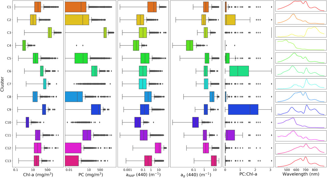
FIGURE 2. Ranges of C_chl, C_pc, a_nap (440), a_g (440), and PC:chl-a for each defined synthetic cluster along with median R_rs spectra. Additional IOP ranges can be found in Supplementary Material.

The 13 clusters were then condensed into seven manually defined OWTs with ecological relevance. Median R_rs spectra of the seven OWTs are shown in Figure 3, where “Mild” represents low to medium biomass mixed blooms (C2, C5, C11), “NAP” represents waters with relatively high non-algal particle loads (C1, C12), “CDOM” represents waters with relatively high CDOM absorption (C8, C13), “Euk” represents eukaryotic algal blooms (C7), “Cy” represents cyanobacteria blooms (C6, C9), “Scum” represents Microcystis floating scum conditions (C3), and “Oligo” represents oligotrophic to slightly mesotrophic waters (C4, C10). The resulting median R_rs spectra from each manually defined OWT are shown in Figure 4 and match exceptionally well with in-situ water types in Kravitz et al. (2020; their Figure 4) for productive South African waters.

FIGURE 3

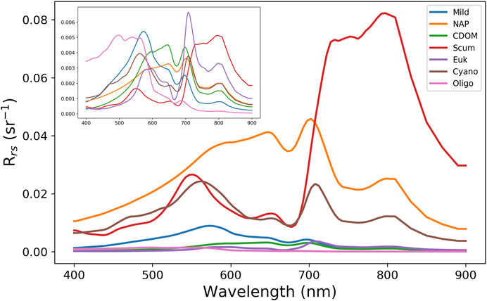
FIGURE 3. Median R_rs spectra of the seven manually defined OWTs derived from the set of 13 clusters. The inset shows the same spectra on a standardized scale, achieved by removing the mean and scaling to unit variance in order to better show shape variation.

FIGURE 4

FIGURE 4. A technical flowchart showing the summarized data development and training stages of ML algorithms to retrieve water quality products (“WQ Products”). S_x indicates one of the seven band configurations used in data preparation. K represents the specific iteration of k-fold cross validation.

Machine Learning Models

K-Nearest Neighbors

The K-nearest neighbor (KNN) algorithm (Altman, 1992) is a non-parametric, lazy learning model, that can be used for regression (KNR) and classification (KNC). The model is “lazy” in that all training data are used in the testing phase. This allows for faster training times, but slower and costlier testing and prediction. The core of the KNN model is based on identifying similarity between datapoints, which is done by calculating distance or proximity of all points to each other, and assuming similar datapoints are close to each other. The model is tuned by choosing the optimal number for K, which defines the number of training samples closest in distance to the new point, followed by a value prediction. How distance between points is calculated can also be defined. KNN has become popular for its simplicity and fast training with minimal tuning; however, predictions take much longer with increasing training data or number of features.

Random Forest

The random forest (RF) algorithm (Ho, 1998; Breiman, 2001) is an extension of the decision tree model, which, in simple terms, constructs a series of yes/no questions about the data until an answer is reached and can be used for classification (RFC) or regression (RFR). RF is an ensemble method that builds tens to thousands of decision trees based on random sampling of training subsets and features, and averages (or majority voting for classification) all the results for a final product. There are a number of tunable hyperparameters that generally differ in how the questions are formed and define the depth of the trees. Training can be computationally expensive with extremely large datasets; however, prediction is much faster than can be achieved using KNN.

XGBoost

The extreme gradient boosting (XGBoost) framework (Chen and Guestrin, 2016) advances the RF model by including gradient boosted decision trees. This ensemble method builds new, weak models sequentially by minimizing errors from previous models and increasing the influence of higher performing models (boosting), until no further model improvements can be made. Gradient boosting then uses the gradient descent algorithm to minimize the loss when adding new models. XGBoost runs exceptionally well on tabulated data for classification or regression purposes and has dominated data science competitions in recent years due to its efficiency and power.

Multi-Layer Perceptron

The multi-layer perceptron (MLP) is a type of classical artificial neural network (ANN) that is capable of learning any non-linear mapping function and can be thought of as a universal approximation algorithm. The fundamental units of MLPs are artificial neurons, each with their own weighting and activation functions. The activation function maps the summed weighted inputs to the output of the neuron. Individual neurons can be merged into networks of neurons, generally in the form of a visible input layer and subsequent hidden layers, including the output layer. The activation function of the output layer constrains the model for the specific type of problem (i.e., regression or classification). With increasing computational resources, deep multi-layer networks composed of multiple layers of hundreds of neurons can now be constructed for highly complex problems.

Cross Validation

Model Inputs and Outputs

The primary input to each ML algorithm is the visible and near infrared channel TOA reflectances or R_rs of the specific sensor and band configuration. The modeled synthetic data were resolved to six multispectral and hyperspectral sensor specifications: Sentinel 3 Ocean and Land Colour Imager (S3-OLCI), Sentinel 2 multi-spectral imager (S2-MSI) at the sensor’s 60, 20, and 10 m band configurations, Landsat 8 operational land imager (L8-OLI), the moderate resolution imaging spectroradiometer (MODIS), and a hypothetical hyperspectral configuration based on the hyperspectral imager for the coastal ocean (HICO). As a means of dimensionality reduction, the seventh configuration consisted of the scores from the first ten EOF modes from a singular value decomposition (SVD) of the entire dataset for HICO bands. In this instance, the ten scores were used as input to the ML model, replacing the channel reflectances. See Table 1 for a list of all sensor band configurations.

TABLE 1

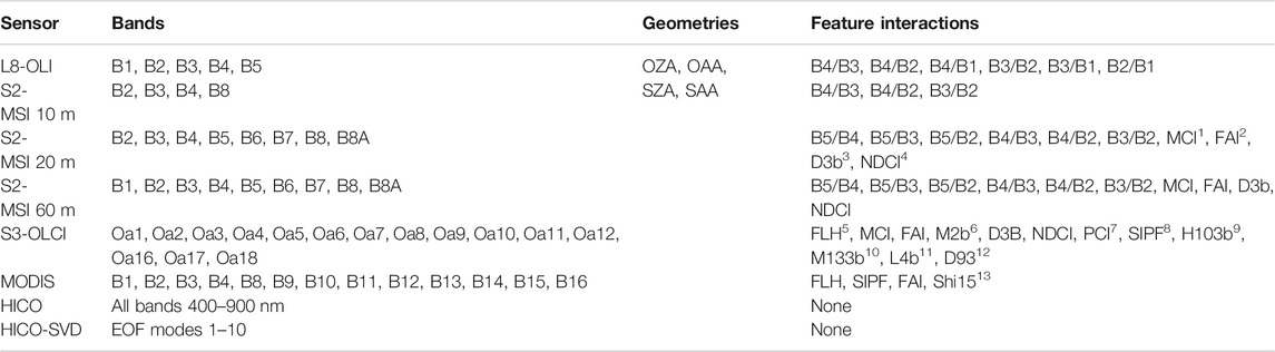
TABLE 1. Inputs for ML models. Inputs are the same for the four ML models used in this study, except for Sun and sensor geometries, which were only used on TOA models. References from 1 to 13 (Gower et al., 2008; Hu, 2009; Dall’Olmo and Gitelson, 2005; Mishra and Mishra, 2012; Gower et al., 1999; Moses et al., 2009; Qi et al., 2014; Matthews et al., 2012; Hunter et al., 2010; Mishra et al., 2013; Liu et al., 2017; Dekker, 1993; Shi et al., 2015):

Inputs to each model consist of three sets of features: 1) the visible and near infrared (NIR) bands of the specific sensor configuration, 2) the Sun and sensor geometry if the model is applied to TOA reflectance, and 3) a selection of feature interactions, which include band ratios and spectral derivative type indices (Table 1). Feature tuning and extraction can have dramatic effects on resulting model errors or accuracies. Generally, interactions among variables can supplement the individual predictor variables to enhance the feature space to improve the predictive capability of the models. This has been confirmed for aquatic cases (Ruescas et al., 2018; Hafeez et al., 2019) where including band interactions such as band ratios or line height models has improved model performance. Model outputs are concentrations of chl-a, PC, and NAP in mg/m³, as well as a_phy in m⁻¹, and the OWT.

The R_rs dataset contains roughly 70,000 samples, while the TOA reflectance dataset contains roughly 260,000 samples. For each dataset, models were evaluated using k-fold cross validation where the data were split into 80% for training and 20% for testing for five folds in order to avoid sampling bias (Figure 4). Performance metrics used in the evaluation consist of both linear and log-transformed root mean squared error (RMSE and RMSELE, respectively), relative RMSE (rRMSE), bias, and median absolute percent error (MAPE).

Hyper-Parameter Tuning

To obtain results of the highest fidelity possible, ML models require optimization of their respective hyper-parameters before training of the actual ML model for product retrieval. The hyper-parameters govern the training process itself and define the model architecture. These parameters are not updated during the learning process and are used to configure the model in various ways. In this study, hyper-parameter tuning was accomplished using a grid search, which builds a model for each possible combination of all hyper-parameters provided, evaluates each model, and selects the architecture with the lowest mean squared error (MSE) for regression models, or accuracy for classification models. The best performing combination of hyper-parameters is then applied to train the ML model using the entire dataset. Computational requirements for extensive hyper-parameter tuning can be very high, especially when dealing with more complex or deep models. The models used here were trained with minimal hyper-parameter tuning, as conducting an exhaustive grid search exercise for every trained model explored in this study would be very computationally expensive. However, a brief hyper-parameter tuning exercise was performed to optimize each of the models’ most sensitive hyperparameters. Final model hyper-parameters are listed in the Supplementary Material. A technical roadmap of the data development and training stages is shown in Figure 4. All the analyses were performed using a personal laptop equipped with 16 GB of RAM.

Results

Surviving L_w at TOA

The average percent contributions of the surviving water signal at L_tot for the seven manually defined OWTs derived above for specific visible and NIR bands are shown in Figure 5. The high inter- and intra-variability of the percent contribution of the L_w signal is evident. Relatively low contribution from the 443 nm band is common amongst OWTs. This region encompasses high amounts of absorption amongst the different aquatic optical constituents as well as significant interference from atmospheric molecular Rayleigh scattering. Consequently, this band only reaches above 20% contribution in extremely scattering conditions containing relatively low amounts of blue absorption due to decreased phytoplankton and CDOM. There is a general increase in surviving aquatic signal with increased inorganic sediment, as well as with a more dominant phytoplankton component. The fraction of L_w at TOA is also relatively elevated in OWTs comprising greater concentrations of PC, particularly the red edge band. When cyanobacteria dominate, L_w at TOA fractions have the potential to reach 40% for red/NIR bands with chl-a concentrations as low as 10 mg/m³, while maxing out at an average of roughly 60% for the 709 nm band just above 100 mg/m³ (data not shown). When eukaryotic algae dominate, average surviving L_w at TOA fraction only exceeds 20% for the NIR bands and at highly elevated chl-a concentrations. This relationship is also apparent when comparing subdued L_w at TOA fractions of the eukaryotic bloom OWT (“Euk”), which represents high biomass eukaryotic algae blooms, vs. the “Cy” OWT dominated by cyanobacteria and containing much higher PC:chl-a ratios (Figure 6). OWTs consisting of relatively high mineral concentrations (“NAP” OWT) yield broadly elevated surviving L_w at TOA, with fractions ranging from 20 to 60% for the green to NIR bands.

FIGURE 5

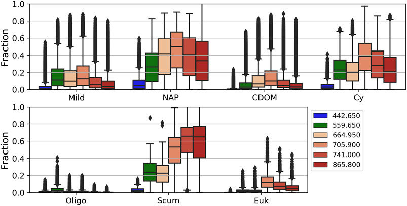
FIGURE 5. Fraction of surviving L_w at L_tot for specific wavelengths for each derived OWT.

FIGURE 6

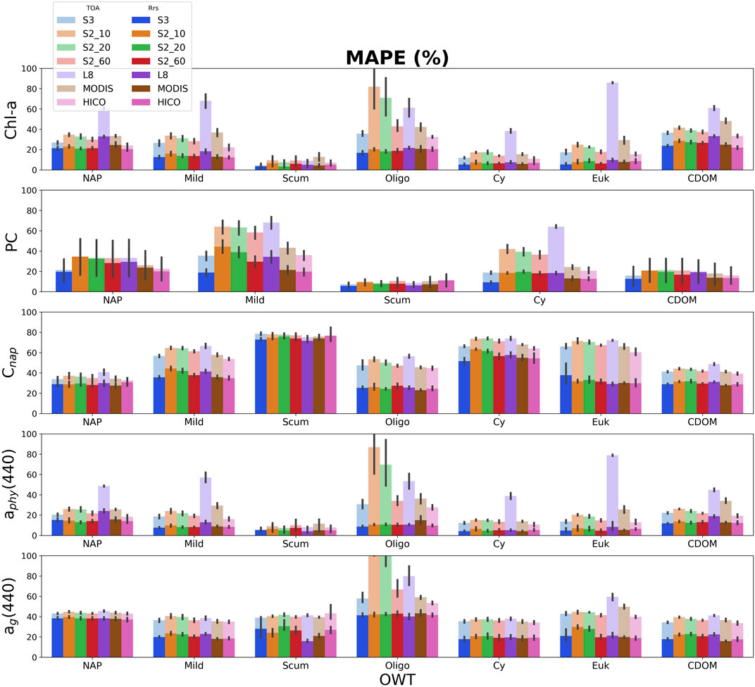
FIGURE 6. Median absolute percent error (MAPE) for MLP derived products (from top-to-bottom: chl-a, PC, and NAP concentrations, absorption of phytoplankton, and a_g at 440 nm). Retrieval errors using R_rs are in solid bright colors, while retrieval errors using TOA reflectance are stacked in corresponding opaque colors. Lower MAPE corresponds to better performance. Error bars represent the standard deviation for the five-fold cross validation.

Model Performance Against Synthetic Dataset

Evaluation of overall model performance applied to TOA reflectance or R_rs spectral data, per sensor, can be found in Supplementary Appendix C for retrieval of chl-a, PC, and NAP concentrations, and a_phy(440). The MLP overwhelmingly outperforms the other ML models in almost every case in terms of MAPE and RMSELE when evaluated against the entire dataset using R_rs data. A lower MAPE/RMSELE would signify better performance (Supplementary Appendix Figure C1). When applied to TOA reflectance, MLP still generally performs the best, although with exceptions in specific cases. The KNR model generally performs the worst for retrievals when applied to both R_rs and TOA reflectance. Considering the variability of these products within the synthetic dataset, the MLP shows promising predictive capabilities for all trophic states.

Figure 6 shows the MAPE of the MLP algorithm retrievals by OWT for each sensor using both R_rs and TOA reflectance data. Significant differences can be observed in the capability of the MLP algorithm for chl-a, PC, and NAP concentration retrievals, as well as retrievals for absorption at 440 nm by phytoplankton and CDOM, due to the different band configurations. The OWT can also significantly affect retrieval performance differently among sensors. When using R_rs data, product retrievals by sensor do not show much intra-variability within OWTs, and on average, yield errors ranging from 20 to 40% amongst OWTs. Exceptions to this include errors >50% for C_nap retrieval, and <20% for chl-a and PC in OWTs dominated by cyanobacteria (Scum and Cy). Phytoplankton absorption at 440 nm is also retrievable with <20% error at R_rs amongst the different band configurations. S3-OLCI shows considerably better retrieval performance of PC than other multi-spectral sensors, in-line with HICO retrieval performance.

Examining product retrieval errors using TOA reflectance by sensor shows more intra-variability within OWTs as compared to R_rs. OWTs that result in lower proportions of surviving L_w signal at TOA, such as the Oligo or Euk water types, experience the greatest difference in product retrieval error when comparing retrievals at R_rs or TOA. When comparing sensor configurations, L8-OLI generally observes the largest discrepancies between product retrievals at R_rs and TOA, most significantly for pigment retrievals and a_phy (440). That said, L8 produces smaller errors at TOA in oligotrophic to mesotrophic waters (Oligo OWT) when compared to the S2-MSI 10 m and 20 m band configurations. Other than for the Oligo OWT, the difference in error between a_g(440) retrievals at R_rs and TOA are relatively consistent between sensor configurations.

Case Study Application

Hartbeespoort Dam, South Africa

To assess the spatial integrity of retrieval products as well as test cross-sensor consistency, a semi-quantitative examination of productive freshwater scenes was undertaken. Figure 7 shows the results of MLP products retrievals using S2-MSI in the 10 m band configuration and L8 TOA reflectances (refer to Table 1 for band configurations). The scene focuses on Hartbeespoort Dam, South Africa, on October 27, 2016. Hartbeespoort Dam is a small, optically complex reservoir that experiences frequent cyanobacteria and floating aquatic macrophyte blooms. The dam is traditionally a very difficult remote sensing target due to its small size and the optically complex nature of the water. While both sensor configurations have similar, limited spectral resolution, L8-OLI provides the advantage of an additional coastal/aerosol band at 440 nm, while S2-MSI at 10 m provides the advantage of a band situated at the red edge of 705 nm. Values of same-day in-situ matchup points for chl-a are overlayed on the product as a qualitative validation. Information regarding sample collection can be found in Kravitz et al. (2020).

FIGURE 7

FIGURE 7. MLP product retrievals over Hartbeespoort Dam on October 27, 2016. The left column shows retrievals using S2 10 m configuration while the right column is the L8 retrievals. All products are derived from TOA reflectance. On the chl-a panels, in-situ sampling points (red dots) are labeled with the station name followed by the measured quantity of chl-a, in units of mg/m³ (e.g., H1--44 indicates station H1 with a measured in-situ chl-a concentration of 44 mg/m³). In-situ data are from Kravitz et al. (2020).

Unfortunately, only in-situ chl-a could be quantified; however, other products are also show to illustrate product relationships (Figure 7). Strong consistency between the two sensor retrievals is apparent. L8 slightly underestimates chl-a outside of the intense bloom in the western part of the dam relative to the S2 retrieval. The PC and a_phy(440) retrievals, although not validated with in-situ data, depict realistic relationships and ranges associated with the chl-a product. Strong consistency between the two sensors is also evident. Inter-comparison of products also depicts the de-coupling of PC and chl-a estimation, as evidenced by strong spatial consistency between chl-a and a_phy(440), while PC is more drastically concentrated in the Western basin, and substantially lower in the Eastern basin. The scene demonstrates the capability for extremely dynamic ranges of water quality product retreivals. Water type classification using the two configurations is also remarkably consistent. Depicting a gradient of scum conditions, to cyanobacteria dominated conditions, to milder sub-surface blooms in the Eastern basin. This can also be visualized in the RGB as fading of the intensity of the green color, where the absorption of the water becomes stronger due to less phytoplankton biomass. S2 appears to differentiate scum and high cyanobacteria concentrations more effectively than L8. This is potentially the result of a combination between the inclusion of the red-edge band utilized for S2, as well as smaller pixel size. AC over intense bloom waters such as these are error prone and can lead to large uncertainties in retrieval products (Kravitz et al., 2020). As the AC and product retrieval are essentially performed together in the inversion, the strong water-leaving signal at TOA allows for very reasonable product retrieval estimates.

Figure 8 displays another instance of same-day chl-a retrievals at Hartbeespoort Dam on March 29, 2017. A large water hyacinth bloom had begun spreading from the North-Eastern basin which can be visualized in the RGB image and is consequently flagged out in product retrievals. This poses a very difficult scenario for medium resolution sensors, with potential for strong signal contamination for less productive water pixels from adjacent bright vegetation pixels. Chl-a product retrieval estimates correlate very well with in-situ measurements, even adjacent to the water hyacinth. Product estimations of C_nap, although not validated with in-situ data, show a realistic de-coupling of organic and inorganic material, with high NAP concentrations displayed in the sediment-laden South Eastern arm of the dam.

FIGURE 8

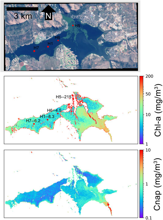
FIGURE 8. MLP product retrievals over Hartbeespoort Dam on March 29, 2017 using L8 TOA reflectance data. For the chl-a panel, in-situ sampling points (red dots) are labeled with the station name followed by the measured quantity of chl-a, in units of mg/m³. In-situ data are from Kravitz et al. (2020).

Lake Erie, United States

A separate semi-quantitative validation of MLP retrieval products was conducted for the western basin of Lake Erie, USA. Figures 9,10 show product retrievals during a mild cyanobacteria bloom on August 13, 2018 using S2 TOA reflectances in the 60 m and 10 m band configurations, respectively. Retrieval products are qualitatively validated with in-situ measurements of chl-a, PC, C_nap, and a_g(440) collected and distributed by the National Oceanographic and Atmospheric Administration (NOAA) Great Lakes Environmental Research Laboratory (GERL) and National Centers for Environmental Information (NCEI) (https://www.glerl.noaa.gov/res/HABs_and_Hypoxia/habsMon.html). Comparison of the two figures demonstrates the capability of multi-parameter inversion using only four bands in the 10 m configuration (Figure 10), while the 60 m configuration uses nine bands in the vis/NIR (Figure 9). Despite the five spectral band difference, product consistency is very strong and respectably correlated with in-situ measurements. The higher spatial resolution in the 10 m configuration also demonstrates the de-coupling of water quality products for a slick of disturbed water emanating from the lower western basin. The high spatial resolution captures the elevated dissolved organic and non-algal content in the disturbed water.

FIGURE 9

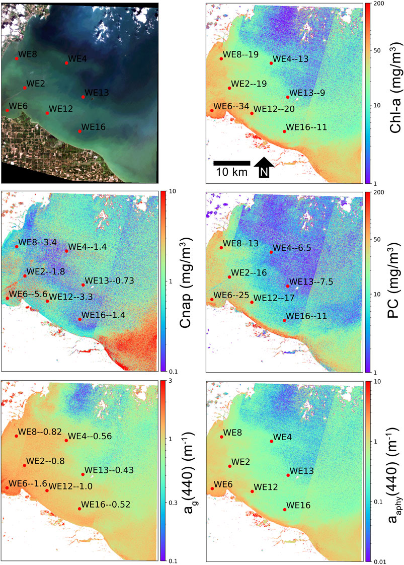
FIGURE 9. MLP product retrievals over the western basin of Lake Erie on August 13, 2018 using S2 60 m band configuration TOA reflectance data. In-situ sampling points (red dots) are labeled with the station name followed by the measured quantity of that particular variable, in units shown on the y-axis. In-situ data are from NOAA GERL and NCEI.

FIGURE 10

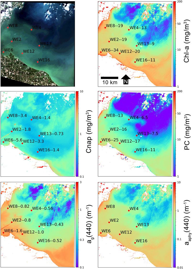
FIGURE 10. MLP product retrievals over the western basin of Lake Erie on August 13, 2018 using S2 10 m band configuration TOA reflectance data. In-situ sampling points (red dots) are labeled with the station name followed by the measured quantity of that particular variable, in units shown on the y-axis. In-situ data are from NOAA GERL and NCEI.

A short time-series analysis was conducted at station WE4 of Lake Erie during the bloom period of 2018 between June and October. In-situ field data are plotted along with product retrievals for S3, S2 in both 10 m and 60 m configurations, and L8, all using TOA reflectance data (Figure 11). All non-cloudy images available for each sensor during the time period were downloaded from either the United States Geological Survey (USGS) Earth Explorer (https://earthexplorer.usgs.gov/), or the European Space Agency (ESA) Copernicus Open Access Hub (https://scihub.copernicus.eu/). Considering the highly dynamic nature of bloom and water dynamics in the western basin, the multi-spectral sensors were able to adequately track the progress of two subsequent cyanobacteria blooms during the time period. Other than some outlying instances of apparent model failure using S3, which would inquire further inspection, Figure 11 demonstrates the capability of a multi-sensor approach to fill temporal gaps due to clouds and revisit times.

FIGURE 11

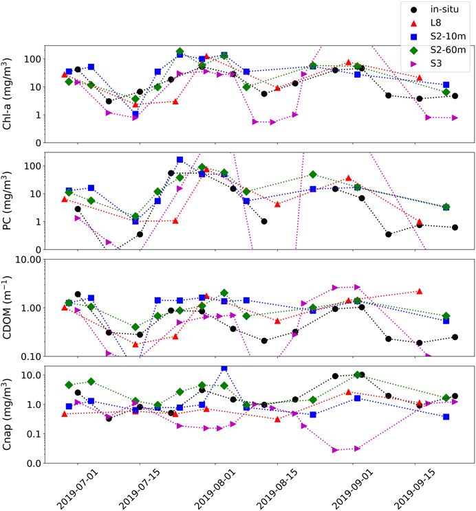
FIGURE 11. Time-series of station WE4 from western Lake Erie. Product retrievals are derived from MLP from S3, S2, and L8 using TOA reflectance data (colors) plotted with in-situ data (black) from NOAA GERL and NCEI.

Figure 12 displays the results of MLP product retrievals using L8-OLI and S2-MSI plotted against same-day in-situ field data for three images of South African waters, which only include chl-a validation, and two images of Lake Erie, which also include PC, a_g(440), and C_nap, for a total of 72 chl-a matchups and 46 matchups for each of PC, a_g(440), and C_nap, totaling 216 total point matchups. Although it is not conventional to aggregate multiple sensors and their associated products, the figure provides an estimation of total error, as calculated using the MAPE, for the three sensor configurations on a limited number of validation points. A combined MAPE of 52% was achieved for the four products at three multi-spectral sensor configurations using TOA reflectance. The error adequately corresponds to results achieved using synthetic data in Figure 6 for these water types, as well as results from other studies using ML trained on in-situ data (Balasubramanian et al., 2020; Pahlevan et al., 2020).

FIGURE 12

FIGURE 12. Measured vs. estimated products; chl-a (N = 72), PC (N = 46), a_g(440) (N = 46), and C_nap (N = 46) for same day matchups from L8 and S2.

Discussion

Machine Learning Models

Four out-of-the-box ML models were trained using synthetic data and applied to EO data using the Python programming language. We note that the aim of this study was not to produce an optimal, finalized retrieval model for operational use, but rather to explore the capacity of a range of well documented ML models to make adequate predictions of water quality variables, trained from synthetic optical and radiometric data. ML has proven an extremely powerful tool that is now more accessible and easier to implement than ever before. This study confirms other reports of ANNs outperforming other “shallow” ML models such as decision trees or support vector machines (SVM) (Peterson et al., 2018; Hafeez et al., 2019). Other ML techniques utilized in recent aquatic work such as feature fusion (Peterson et al., 2019) were also implemented to a degree in this study. Multiple “feature interactions” in the form of band ratios or line height indices were included in model training along with sensor visible and NIR bands. Ruescas et al. (2018) found increasing model performance by including more feature interactions for a ML model for CDOM retrieval. Although the results are not shown here, we trained a subset of ML models with and without the inclusion of feature interactions; the significant increase in performance when feature interactions were included led us to include them for all models.

Pahlevan et al. (2020) and Balasubramanian et al. (2020) found that a mixture density network (MDN), which is essentially an ANN with the final layer mapped to a mixture of distributions, produced extremely robust results for chl-a and suspended solid material. MDNs would theoretically be the optimal choice for aquatic parameter retrievals, as one can design a highly efficient deep neural network (DNN) while also addressing the signal ambiguity problem of optical remote sensing through the addition of a mixture of parameterized Gaussians. Such an approach was attempted here; however, it took considerably longer for training and cross validation, and produced roughly similar results to the MLP model, such that it was discarded. Future work, with access to higher computational resources, should include training of deeper NNs and the inclusion of mixture distributions.

Shallow ML models such as Random Forest and XGBoost require far less parameterization and computational resources but still provide relatively robust results. We note that all models were both trained and validated using mainly the synthetic database with only the MLP model validated against a limited in-situ dataset. Future work will entail validating products against available in-situ data. It is speculated that performance will decline somewhat when validated against field data due to spatial inconsistencies and uncertainty introduced by field methods.

Product Consistency

Pahlevan et al. (2020) note AC to still be one of the major challenges for operational inland and coastal remote sensing. The present study explores the capability of product retrievals from TOA reflectances. We find that water types for turbid or productive inland waters have substantially higher percentages of surviving water-leaving radiances reaching the satellite sensor than oligotrophic waters or waters dominated by eukaryotic algae (Figure 5). The separation of MLP performance by OWT confirms that water types with stronger bulk scattering signals have smaller discrepancy between product retrievals from TOA reflectance and R_rs (Figure 6). An OWT based framework could be used to run AC only on oligotrophic pixels where AC processors are more ideally suited, with product retrievals made from TOA in more productive or scattering water types. Due to uncertainties inherent to current AC processors, especially for smaller water bodies, the product maps shown here (e.g., Figures 7–10) were made using TOA reflectance data. Nevertheless, promising AC processors have been developed using a combined synthetic data/NN approach (Fan et al., 2017), and the dataset developed here could be used in future to train an appropriate AC.

The water bodies shown in this manuscript have the potential to experience high spatial and temporally dynamic blooms. Sensor requirements for operational monitoring of such waters are recommended to be <60 m spatial resolution with daily to tri-weekly revisit times (Hestir et al., 2015; Mouw et al., 2015; Muller-Karger et al., 2018). The case studies presented in Case Study Application Section demonstrate the fine-scale spatial distributions of cyanobacteria blooms. MLP products at different spatial resolutions demonstrate how spatial smoothing from just 10–60 m can cause significant differences in product retrievals. Reasonable comparisons of in-situ data against highly consistent product maps between S2 10 m and 60 m configurations provide a promising justification of the capability of ML to exploit information from just a few sensor bands. Extreme temporal dynamics can additionally be visualized in the short time-series shown in Figure 11, where a multi-sensor approach was adequately able to trace fine temporal dynamics of cyanobacteria blooms in Lake Erie.

Product Integrity

The magnitude and fraction of the water-leaving radiance surviving to TOA can also have a significant impact on the resulting sensor signal-to-noise ratio (SNR). There is a trade-off in sensor design concerning spatial and spectral resolution and resulting sensor radiometric quality. For example, sensor configurations such as S2-MSI or L8-OLI sacrifice SNR for the sake of higher spatial resolution. Narrower band widths can also compromise SNR. Numerous investigations have concluded that errors in both AC and geophysical retrievals only become acceptable (<100%) at SNRs of 300 – 500 at visible wavelengths and >100 at NIR wavelengths for water quality applications (Moses et al., 2015; Wang and Gordon, 2018; Qi et al., 2017; Jorge et al., 2017). Some studies suggest SNR for NIR bands to be >600 if used in AC schemes (Wang and Gordon, 2018; Qi et al., 2017). A brief examination of typical SNR values for S2-MSI for the OWTs defined here is presented in Figure 13. The SNR in this instance applies solely to the water-leaving radiance reaching TOA (L_w) rather than to the total radiance signal at TOA, which includes the atmosphere (L_tot), that the aforementioned studies primarily use. Using SNR for L_w provides an SNR more relevant to the investigator as it pertains directly to the signal of interest (Kudela et al., 2019). Kudela et al. (2019) proposed a set of theoretical SNR thresholds described as a theoretical research limit (SNR = 2), a theoretical validation limit (SNR = 8), and a theoretical calibration limit (SNR = 50). The SNR ranges depicted in Figure 13 follow similar patterns and relationships as in Figure 5 for that of surviving L_w at TOA. Only water types with a strong bulk scattering signal such as cyanobacteria- or NAP dominated waters appear to reach a theoretical validation limit of 8, on average (Figure 13). Waters types with more subdued signal strength have difficulty reaching even a theoretical research limit of SNR of 2 in visible bands. Thus, unless dealing with extremely scattering waters, MSI SNRs are considerably lower than the recommended radiometric requirements for aquatic application, which can lead to large uncertainties in product retrieval. The synthetic dataset approach could be used in future to perform robust sensor and algorithm specific uncertainty analysis per OWT.

FIGURE 13

FIGURE 13. SNR for water-leaving radiance (L_w) for S2-MSI developed using the ESA Sentinel 2 radiometric uncertainty tool (Gorroño et al., 2017; 2018) for the OWTs defined in this study. The black, red, and blue dashed lines represent the theoretical research, validation, and calibration limits described in Kudela et al. (2019).

The adjacency effect (AE), whereby strong spatial heterogeneity from surrounding terrestrial sources contaminates the water signal, has the potential to induce considerable errors in retrieved products (Bulgarelli et al., 2017). Contamination by green terrestrial vegetation at TOA was incorporated into the synthetic modeling in an attempt to mitigate this issue. Figure 14 shows an S2 scene over a small dam in South Africa that was found to be affected by considerable adjacency by Kravitz et al. (2020). The predicted contribution of adjacency to water pixels based on a simple RF model trained using the synthetic dataset is illustrated. The plot shows realistic gradation of increasing adjacency contribution towards the edges of the dam in the darker waters, as well as in instances near bright surface cyanobacteria blooms. Areas of intense algal surface bloom would be less affected by green vegetation adjacency since they exhibit similar reflectance patterns in the red and NIR, and would themselves be potentially contaminating nearby “less bright” water pixels. While more quantitative validation is required, the fact that the model demonstrates reasonable patterns of the AE gives confidence that other retrieval products would be inherently corrected for this effect. Future work should incorporate more sources of adjacency and could also include other sources of signal contamination such as Sun glint.

FIGURE 14

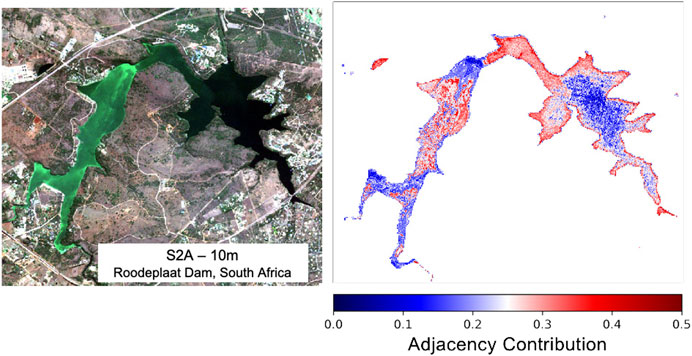
FIGURE 14. Percent adjacency contribution derived using RF regression over Roodeplaat Dam, South Africa, using TOA reflectance data.

Outlook

While this study is more proof-of-concept than finalized product, the results suggest the potential for using a synthetic dataset and ML approach to develop operational global freshwater monitoring products. Expansion of the synthetic dataset by incorporating more diverse phytoplankton IOPs and other sources of signal contamination is the logical next step. While the amount of synthetic data generated here (∼260,000 TOA spectra) is quite small with respect to current advances in Big Data analytics, the development of extremely large synthetic datasets containing tens and hundreds of millions of datapoints from which advanced deep learning networks can be trained, would be feasible with access to high powered computing resources. Validation of models using global in-situ datasets would then be the final step to compare product outputs trained from synthetic data to outputs trained on field data as in Pahlevan et al. (2020) and Balasubramanian et al. (2020). That said, it is very promising that the model performance described here relates so well to the results detailed in the aforementioned studies. Further research should also include parameterized sensitivity studies identifying the most optimal spectral and radiometric resolutions that ML can exploit. Having a large, high quality synthetic dataset would also be an asset for sensitivity studies pertaining to upcoming satellite missions such as NASA’s Surface, Biology, and Geology (SBG) mission.

This study suggests that both L8 and S2 at its various sensor configurations contain enough spectral information at TOA, to produce reasonable estimates of various aquatic products for productive water bodies. Highly consistent product outputs were found for S2 at 60 m and 10 m resolutions, which is significant considering the five additional NIR spectral bands in the 60 m configuration. This observation has potential implications for future sensor design as it suggests that more resources could be invested in increasing SNR or spatial resolutions of sensors while spectral resolution remains fairly low, at least for the water types investigated here. Finally, our findings suggest that relevant bands for assessing wide ranging trophic levels should at least include a short wavelength blue band around 440 nm as in L8 for more oligotrophic instances and highly absorbing scenarios, a band around 620 nm to aid in cyanobacteria detection and quantification, and a band in the red edge around 710 nm to capture the phytoplankton scattering peak.

Conclusion

A state-of-the-art synthetic dataset of R_rs and at-sensor reflectances for various sensor configurations with coincident measurements of associated IOPs and optical constituent concentrations was developed using novel techniques suited to high biomass, complex optical systems and cyanobacteria dominated waters. The parameterization of the RTM describing the synthetic dataset utilizes our most current understanding of optical properties and relationships related to eutrophic and cyanobacteria dominated waters and includes four prominent novel aspects: 1) two-layered, size and type-specific phytoplankton IOPs; 2) mixed assemblage chl-a fluorescence; 3) assemblage based modeled PC concentrations; and 4) paired sensor-specific TOA reflectances, which includes green vegetation adjacency. R_rs spectra modeled through the RTM were compiled into 13 distinct clusters using a functional data analysis and k-means clustering approach, and the 13 clusters were then condensed into seven manually defined OWTs. The water types are similar to those discovered using in-situ data by Spyrakos et al. (2018) and Kravitz et al. (2020). Manual inspection of synthetic OWTs showed relationships and ranges in the concentrations of water constituents and IOPs that were similar to in-situ derived OWTs. Four types of current ML architectures were tested and trained using the synthetic dataset. Major points of interest resulting from the training and application of machine learning models in this study can be summarized as follows:

1. Surviving L_w fraction at TOA is significantly increased by increased bulk scattering such as in NAP or cyanobacteria dominated waters.

2. An artificial neural network produced the most promising results among all sensors and retrieval products when compared to other machine learning methods.

3. The 620 nm band of OLCI, which aligns with the maximum absorption peak of PC, appears to provide a significant advantage over other multispectral sensors for the quantification of cyanobacteria.

4. The 443 nm band present in L8-OLI, but not in the S2-MSI 10 m and 20 m configurations, appears to aid significantly in pigment retrieval in oligotrophic waters.

5. The red-edge band, present in MSI and OLCI, aids significantly in pigment retrieval in bloom waters.

6. Water types containing higher fractions of surviving L_w at TOA experience significantly smaller differences in product retrieval errors when comparing retrieval results from TOA reflectance and R_rs.

7. Application to EO imagery provides realistic concentration gradients of chl-a, PC, NAP, and absorption due to CDOM at 440 nm for wide ranging trophic scenarios for small inland water bodies using TOA reflectance data, corroborated by in-situ field data.

8. Product retrievals from low spectral resolution configurations such as L8-OLI and S2-MSI at 10 m resolution produce as consistent results as product retrievals from higher spectral resolution configurations such as S2-MSI at 60 m, OLCI, and MODIS.

With a combination of current and past sensor spatial resolutions ranging from 10 m to 4 km scales, a synergistic evaluation of water constituents, with known uncertainties by OWT, may assist in improving global-scale capability for monitoring fine scale ecological dynamics of coastal and inland waters. The synthetic dataset produced and interrogated here represents the first step towards this goal. It is by no means an exhaustive compilation of all possible natural values and relationships found in inland waters; however, it works as a proof-of-concept to show the capability of these techniques for creating accurate simulations of real-world aquatic environments.

Data Availability Statement

The raw data supporting the conclusion of this article will be made available by the authors, without undue reservation.

Author Contributions

JK: Conceptualization, Methodology, Software, Formal Analysis, Investigation, Data Curation, Writing - Original Draft, Writing - Review and Editing, Visualization, Project Administration, MM: Resources, Writing - Review and Editing, Supervision, Funding acquisition, SB: Resources, Supervision, Funding Acquisition, LL: Software, Writing- Review and Editing, Supervision, SF: Supervision, Funding Acquisition.

Funding

Financial support for this project was provided through the South Africa Water Research Commission Grant K5/2518 and Grant K5/2458, NRF SANAP Grant 105539 and 110735, UCT Vice Chancellor's Future Leaders 2030 Award, and Royal Society/African Academy of Sciences Future Leaders-Africa Independent Researcher Fellowship.

Conflict of Interest

Author MM was employed by the company CyanoLakes (Pty) Ltd.

The remaining authors declare that the research was conducted in the absence of any commercial or financial relationships that could be construed as a potential conflict of interest.

Supplementary Material

The Supplementary Material for this article can be found online at: https://www.frontiersin.org/articles/10.3389/fenvs.2021.587660/full#supplementary-material.

References

Altman, N. S. (1992). An introduction to kernel and nearest-neighbor nonparametric regression. Am. Stat. 46 (3), 175–185. doi:10.1080/00031305.1992.10475879

CrossRef Full Text | Google Scholar

Arabi, B., Salama, M., Wernand, M., and Verhoef, W. (2016). MOD2SEA: a coupled atmosphere-hydro-optical model for the retrieval of chlorophyll-a from remote sensing observations in complex turbid waters. Remote Sensing 8 (9), 722. doi:10.3390/rs8090722

CrossRef Full Text | Google Scholar

Babin, M., Morel, A., and Gentili, B. (1996). Remote sensing of sea surface sun-induced chlorophyll fluorescence: consequences of natural variations in the optical characteristics of phytoplankton and the quantum yield of chlorophyll a fluorescence. Int. J. ;Remote Sensing 17 (12), 2417–2448. doi:10.1080/01431169608948781

CrossRef Full Text | Google Scholar

Balasubramanian, S. V., Pahlevan, N., Smith, B., Binding, C., Schalles, J., Loisel, H., et al. (2020). Robust algorithm for estimating total suspended solids (TSS) in inland and nearshore coastal waters, Remote Sensing Environ., 246, 111768. doi:10.1016/j.rse.2020.111768

CrossRef Full Text | Google Scholar

Ball, J. E., Anderson, D. T., and Chan, C. S. (2017). Comprehensive survey of deep learning in remote sensing: theories, tools, and challenges for the community. J. Appl. Remote Sensing 11 (4), 042609. doi:10.1117/1.jrs.11.042609

CrossRef Full Text | Google Scholar

Beaulieu, J. J., DelSontro, T., and Downing, J. A. (2019). Eutrophication will increase methane emissions from lakes and impoundments during the 21st century. Nat. Commun. 10 (1), 1–5. doi:10.1038/s41467-019-09100-5

PubMed Abstract | CrossRef Full Text | Google Scholar

Behrenfeld, M. J., Westberry, T. K., Boss, E. S., O'Malley, R. T., Siegel, D. A., Wiggert, J. D., et al. (2009). Satellite-detected fluorescence reveals global physiology of ocean phytoplankton. Biogeosciences 6 (5), 779. doi:10.5194/bg-6-779-2009

CrossRef Full Text | Google Scholar

Bernard, S., Probyn, T. A., and Quirantes, A. (2009). Simulating the optical properties of phytoplankton cells using a two-layered spherical geometry. Biogeosci. Discuss. 6 (1).

Google Scholar

Bernard, S., Shillington, F. A., and Probyn, T. A. (2007). The use of equivalent size distributions of natural phytoplankton assemblages for optical modeling. Opt. Exp. 15 (5), 1995–2007.

Bidigare, R. R., Ondrusek, M. E., Morrow, J. H., and Kiefer, D. A. (1990). In-vivo absorption properties of algal pigments. Int. Soc. Opt. Photon. 1302, 290–302.

Google Scholar

Binding, C. E., Greenberg, T. A., and Bukata, R. P. (2011). Time series analysis of algal blooms in Lake of the Woods using the MERIS maximum chlorophyll index. J. Plankton Res. 33 (12), 1847–1852. doi:10.1093/plankt/fbr079

CrossRef Full Text | Google Scholar

Blondeau-Patissier, D., Gower, J. F. R., Dekker, A. G., Phinn, S. R., and Brando, V. E. (2014). A review of ocean color remote sensing methods and statistical techniques for the detection, mapping and analysis of phytoplankton blooms in coastal and open oceans. Prog. Oceanogr. 123, 123–144. doi:10.1016/j.pocean.2013.12.008

CrossRef Full Text | Google Scholar

Breiman, L. (2001). Random forests. Machine Learn. 45 (1), 5–32. doi:10.1023/a:1010933404324

CrossRef Full Text | Google Scholar

Brewin, R. J. W., Tilstone, G. H., Jackson, T., Cain, T., Miller, P. I., Lange, P. K., et al. (2017). Modelling size-fractionated primary production in the Atlantic Ocean from remote sensing. Prog. Oceanogr. 158, 130–149. doi:10.1016/j.pocean.2017.02.002

CrossRef Full Text | Google Scholar

Bricaud, A., Roesler, C., and Zaneveld, J. R. V. (1995). In situ methods for measuring the inherent optical properties of ocean waters. Limnol. Oceanogr. 40 (2), 393–410. doi:10.4319/lo.1995.40.2.0393

CrossRef Full Text | Google Scholar

Brockmann, C., Doerffer, R., Peters, M., Kerstin, S., Embacher, S., and Ruescas, A. (2016). Evolution of the C2RCC neural network for Sentinel 2 and 3 for the retrieval of ocean colour products in normal and extreme optically complex waters. Living Planet. Symp. 740 (54), 393.

Google Scholar

Bukata, R. P. (1995). The effects of chlorophyll, suspended mineral, and dissolved organic carbon on volume reflectance. Opt. Prop. Remote Sensing 64, 135–166.

Google Scholar

Bulgarelli, B., Kiselev, V., and Zibordi, G. (2017). Adjacency effects in satellite radiometric products from coastal waters: a theoretical analysis for the northern Adriatic Sea. Appl. Opt. 56 (4), 854–869. doi:10.1364/ao.56.000854

PubMed Abstract | CrossRef Full Text | Google Scholar

Bulgarelli, B., Kiselev, V., and Zibordi, G. (2014). Simulation and analysis of adjacency effects in coastal waters: a case study. Appl. Opt. 53 (8), 1523–1545. doi:10.1364/ao.53.001523

PubMed Abstract | CrossRef Full Text | Google Scholar

Carlson, R. E., and Simpson, J. (1996). A coordinator’s guide to volunteer lake monitoring methods, North Am. Lake Manag. Soc. 96. 305.

Google Scholar

Chen, T., and Guestrin, C. (2016). Xgboost: a scalable tree boosting system, in Proceedings of the 22nd ACM SIGKDD international conference on knowledge discovery and data mining, 785–794.

Google Scholar

Dall'Olmo, G., and Gitelson, A. A. (2006). Effect of bio-optical parameter variability and uncertainties in reflectance measurements on the remote estimation of chlorophyll-a concentration in turbid productive waters: modeling results. Appl. Opt. 45 (15), 3577–3592. doi:10.1364/ao.45.003577

PubMed Abstract | CrossRef Full Text | Google Scholar

Dall’Olmo, G., and Gitelson, A. A. (2005). Effect of bio-optical parameter variability on the remote estimation of chlorophyll-a concentration in turbid productive waters: experimental results. Appl. Opt. 44 (3), 412–422.

PubMed AbstractGoogle Scholar

Dekker, A. G. (1993). Detection of optical water quality parameters for eutrophic waters by high resolution remote sensing.

Doerffer, R., and Schiller, H. (2008). MERIS lake water algorithm for BEAM—MERIS algorithm theoretical basis document. V1.0, 10 June 2008. Geesthacht, Germany: GKSS Research Center.

D. R. Mishra, I. Ogashawara, and A. A. Gitelson (2017). in Bio-optical modeling and remote sensing of inland waters (New York, NY: Elsevier).

Evers-King, H., Bernard, S., Lain, L. R., and Probyn, T. A. (2014). Sensitivity in reflectance attributed to phytoplankton cell size: forward and inverse modelling approaches. Opt. Expr. 22 (10), 11536–11551. doi:10.1364/oe.22.011536

CrossRef Full Text | Google Scholar

Fan, Y., Li, W., Gatebe, C. K., Jamet, C., Zibordi, G., Schroeder, T., et al. (2017). Atmospheric correction over coastal waters using multilayer neural networks. Rem. Sensing Environ. 199, 218–240. doi:10.1016/j.rse.2017.07.016

CrossRef Full Text | Google Scholar

Fischer, J., and Kronfeld, U. (1990). Sun-stimulated chlorophyll fluorescence 1: influence of oceanic properties. Int. J. Remote Sensing 11 (12), 2125–2147. doi:10.1080/01431169008955166

CrossRef Full Text | Google Scholar

Ganf, G., Oliver, R., and Walsby, A. (1989). Optical properties of gas-vacuolate cells and colonies of Microcystis in relation to light attenuation in a turbid, stratified reservoir (Mount Bold Reservoir, South Australia). Mar. Freshw. Res. 40 (6), 595–611. doi:10.1071/mf9890595

CrossRef Full Text | Google Scholar

Gholizadeh, M., Melesse, A., and Reddi, L. (2016). A comprehensive review on water quality parameters estimation using remote sensing techniques. Sensors 16 (8), 1298. doi:10.3390/s16081298

CrossRef Full Text | Google Scholar

Ghorbanzadeh, O., Blaschke, T., Gholamnia, K., Meena, S., Tiede, D., and Aryal, J. (2019). Evaluation of different machine learning methods and deep-learning convolutional neural networks for landslide detection. Remote Sensing 11 (2), 196. doi:10.3390/rs11020196

CrossRef Full Text | Google Scholar

Gilerson, A., Zhou, J., Hlaing, S., Ioannou, I., Amin, R., Gross, B., et al. (2007). Fluorescence contribution to reflectance spectra for a variety of coastal waters. Coast. Ocean Rem. Sensing 6680, 66800C.

Google Scholar

Gilerson, A., Zhou, J., Hlaing, S., Ioannou, I., Gross, B., Moshary, F., et al. (2008). Fluorescence component in the reflectance spectra from coastal waters. II. Performance of retrieval algorithms. Opt. Express 16 (4), 2446–2460. doi:10.1364/oe.16.002446

PubMed Abstract | CrossRef Full Text | Google Scholar

Gorroño, J., Fomferra, N., Peters, M., Gascon, F., Underwood, C., Fox, N., et al. (2017). A radiometric uncertainty tool for the Sentinel 2 mission. Rem. Sensing 9 (2), 178. doi:10.3390/rs9020178

CrossRef Full Text | Google Scholar

Gorroño, J., Hunt, S., Scanlon, T., Banks, A., Fox, N., Woolliams, E., et al. (2018). Providing uncertainty estimates of the Sentinel-2 top-of-atmosphere measurements for radiometric validation activities. Eur. J. Remote Sensing 51 (1), 650–666. doi:10.1080/22797254.2018.1471739

CrossRef Full Text | Google Scholar

Govindjee, G. (2004). Chlorophyll a fluorescence: a bit of basics and history. Chlorophyll a fluorescence: a signature of photosynthesis. Dordrecht: Springer, 1–42.

Gower, J. F. R., Doerffer, R., and Borstad, G. A. (1999). Interpretation of the 685nm peak in water-leaving radiance spectra in terms of fluorescence, absorption and scattering, and its observation by MERIS. Int. J. Remote Sensing 20 (9), 1771–1786. doi:10.1080/014311699212470

CrossRef Full Text | Google Scholar

Gower, J., King, S., and Goncalves, P. (2008). Global monitoring of plankton blooms using MERIS MCI. Int. J. Remote Sensing 29 (21), 6209–6216. doi:10.1080/01431160802178110

CrossRef Full Text | Google Scholar

Greene, R. M., Geider, R. J., Kolber, Z., and Falkowski, P. G. (1992). Iron-induced changes in light harvesting and photochemical energy conversion processes in eukaryotic marine algae. Plant Physiol. 100 (2), 565–575. doi:10.1104/pp.100.2.565

PubMed Abstract | CrossRef Full Text | Google Scholar

Hafeez, S., Wong, M., Ho, H., Nazeer, M., Nichol, J., Abbas, S., et al. (2019). Comparison of machine learning algorithms for retrieval of water quality indicators in case-II waters: a case study of Hong Kong. Remote Sensing 11 (6), 617. doi:10.3390/rs11060617

CrossRef Full Text | Google Scholar

Hestir, E. L., Brando, V. E., Bresciani, M., Giardino, C., Matta, E., Villa, P., et al. (2015). Measuring freshwater aquatic ecosystems: the need for a hyperspectral global mapping satellite mission. Rem. Sensing Environ. 167, 181–195. doi:10.1016/j.rse.2015.05.023

CrossRef Full Text | Google Scholar

Hieronymi, M., Müller, D., and Doerffer, R. (2017). The OLCI Neural Network Swarm (ONNS): a bio-geo-optical algorithm for open ocean and coastal waters. Front. Mar. Sci. 4, 140. doi:10.3389/fmars.2017.00140

CrossRef Full Text | Google Scholar

Ho, J. C., Michalak, A. M., and Pahlevan, N. (2019). Widespread global increase in intense lake phytoplankton blooms since the 1980s. Nature, 574, 667. doi:10.1038/s41586-019-1648-7

PubMed Abstract | CrossRef Full Text | Google Scholar

Ho, T. K. (1998). The random subspace method for constructing decision forests. IEEE Trans. Pattern Anal. Mach. Intell. 20 (8), 832–844.

Google Scholar

Hu, C. (2009). A novel ocean color index to detect floating algae in the global oceans. Rem. Sensing Environ. 113 (10), 2118–2129. doi:10.1016/j.rse.2009.05.012

CrossRef Full Text | Google Scholar

Hu, C., Chen, Z., Clayton, T. D., Swarzenski, P., Brock, J. C., and Muller–Karger, F. E. (2004). Assessment of estuarine water-quality indicators using MODIS medium-resolution bands: initial results from Tampa Bay, FL. Rem. Sensing Environ. 93 (3), 423–441. doi:10.1016/j.rse.2004.08.007

CrossRef Full Text | Google Scholar

Hunter, P. D., Tyler, A. N., Carvalho, L., Codd, G. A., and Maberly, S. C. (2010). Hyperspectral remote sensing of cyanobacterial pigments as indicators for cell populations and toxins in eutrophic lakes. Rem. Sensing Environ. 114 (11), 2705–2718. doi:10.1016/j.rse.2010.06.006

CrossRef Full Text | Google Scholar

Huot, Y., Brown, C. A., and Cullen, J. J. (2005). New algorithms for MODIS sun-induced chlorophyll fluorescence and a comparison with present data products. Limnol. Oceanogr. Methods 3 (2), 108–130. doi:10.4319/lom.2005.3.108

CrossRef Full Text | Google Scholar

Huot, Y., Brown, C. A., and Cullen, J. J. (2007). Retrieval of phytoplankton biomass from simultaneous inversion of reflectance, the diffuse attenuation coefficient, and Sun-induced fluorescence in coastal waters. J. Geophys. Res. Oceans 112 (C6), 94. doi:10.1029/2006jc003794

CrossRef Full Text | Google Scholar

Johnsen, G., and Sakshaug, E. (2007). Biooptical characteristics of PSII and PSI in 33 species (13 pigment groups) of marine phytoplankton, and the relevance for pulse-amplitude-modulated and fast-repetition-rate fluorometry 1. J. Phycol. 43 (6), 1236–1251. doi:10.1111/j.1529-8817.2007.00422.x

CrossRef Full Text | Google Scholar

Jorge, D. S., Barbosa, C. C., De Carvalho, L. A., Affonso, A. G., Lobo, F. D. L., and Novo, E. M. D. M. (2017). Snr (signal-to-noise ratio) impact on water constituent retrieval from simulated images of optically complex amazon lakes. Remote Sens. 9 (7), 644.

Jupp, D., Kirk, J., and Harris, G. (1994). Detection, identification and mapping of cyanobacteria—using remote sensing to measure the optical quality of turbid inland waters. Mar. Freshw. Res. 45 (5), 801–828. doi:10.1071/mf9940801

CrossRef Full Text | Google Scholar

Kravitz, J., Matthews, M., Bernard, S., and Griffith, D. (2020). Application of Sentinel 3 OLCI for chl-a retrieval over small inland water targets: successes and challenges. Remote Sensing Environ. 237, 111562. doi:10.1016/j.rse.2019.111562

CrossRef Full Text | Google Scholar

Kudela, R. M., Hooker, S. B., Houskeeper, H. F., and McPherson, M. (2019). The influence of signal to noise ratio of legacy airborne and satellite sensors for simulating next-generation coastal and inland water products. Remote Sensing 11 (18), 2071. doi:10.3390/rs11182071

CrossRef Full Text | Google Scholar

Kutser, T., Metsamaa, L., and Dekker, A. G. (2008). Influence of the vertical distribution of cyanobacteria in the water column on the remote sensing signal. Coast. Shelf Sci. 78 (4), 649–654. doi:10.1016/j.ecss.2008.02.024

CrossRef Full Text | Google Scholar

Kutser, T., Metsamaa, L., Strömbeck, N., and Vahtmäe, E. (2006). Monitoring cyanobacterial blooms by satellite remote sensing. Estuarine Coast. Shelf Sci. 67 (1‐2), 303–312.

Kutser, T. (2004). Quantitative detection of chlorophyll in cyanobacterial blooms by satellite remote sensing. Limnol. Oceanogr. 49 (6), 2179–2189. doi:10.4319/lo.2004.49.6.2179

CrossRef Full Text | Google Scholar

Kutser, T., Soomets, T., Toming, K., Uiboupin, R., Arikas, A., Vahter, K., et al. (2018). Assessing the Baltic sea water quality with Sentinel-3 OLCI imagery, in 2018 IEEE/OES Baltic International Symposium (BALTIC), IEEE, 1–6.

Google Scholar

Lain, L., and Bernard, S. (2018). The fundamental contribution of phytoplankton spectral scattering to ocean colour: implications for satellite detection of phytoplankton community structure. Appl. Sci. 8 (12), 2681. doi:10.3390/app8122681

CrossRef Full Text | Google Scholar

Lain, L. R., Bernard, S., and Evers-King, H. (2014). Biophysical modelling of phytoplankton communities from first principles using two-layered spheres: equivalent Algal Populations (EAP) model. Opt. express 22 (14), 16745–16758.

PubMed Abstract | CrossRef Full Text | Google Scholar

Lain, L. R., Bernard, S., and Matthews, M. W. (2016). Biophysical modelling of phytoplankton communities from first principles using two-layered spheres: equivalent Algal Populations (EAP) model: erratum. Opt. Express 24 (24), 27423–27424. doi:10.1364/oe.24.027423

PubMed Abstract | CrossRef Full Text | Google Scholar

Lee, Z. P. (2003). Models, parameters, and approaches that used to generate wide range of absorption and backscattering spectra. Ocean Color Algorithm Working Group IOCCG. doi:10.1920/wp.cem.2003.1303

CrossRef Full Text | Google Scholar

Lee, Z. (2006). Remote sensing of inherent optical properties: fundamentals, tests of algorithms, and applications.

Li, L., Li, L., and Song, K. (2015). Remote sensing of freshwater cyanobacteria: an extended IOP Inversion Model of Inland Waters (IIMIW) for partitioning absorption coefficient and estimating phycocyanin. Remote Sensing Environ. 157, 9–23. doi:10.1016/j.rse.2014.06.009

CrossRef Full Text | Google Scholar

Li, Y., Zhang, H., Xue, X., Jiang, Y., and Shen, Q. (2018). Deep learning for remote sensing image classification: a survey. WIREs Data Min. Knowl. Discov. 8 (6), e1264. doi:10.1002/widm.1264

CrossRef Full Text | Google Scholar

Liu, G., Simis, S. G., Li, L., Wang, Q., Li, Y., Song, K., et al. (2017). A four-band semi- analytical model for estimating phycocyanin in inland waters from simulated MERIS and OLCI data. IEEE Trans. Geosci. Remote Sensing 56 (3), 1374–1385.

Google Scholar

Lu, Y., Li, L., Hu, C., Li, L., Zhang, M., Sun, S., et al. (2016). Sunlight induced chlorophyll fluorescence in the near-infrared spectral region in natural waters: interpretation of the narrow reflectance peak around 761 nm. J. Geophys. Res. Oceans 121 (7), 5017–5029. doi:10.1002/2016jc011797

CrossRef Full Text | Google Scholar

Ma, L., Liu, Y., Zhang, X., Ye, Y., Yin, G., and Johnson, B. A. (2019). Deep learning in remote sensing applications: a meta-analysis and review. ISPRS J. Photogram. Rem. sensing 152, 166–177. doi:10.1016/j.isprsjprs.2019.04.015

CrossRef Full Text | Google Scholar

Martins, V., Barbosa, C., de Carvalho, L., Jorge, D., Lobo, F., and Novo, E. (2017). Assessment of atmospheric correction methods for Sentinel-2 MSI images applied to Amazon floodplain lakes. Rem. Sensing 9 (4), 322. doi:10.3390/rs9040322

CrossRef Full Text | Google Scholar

Matthews, M., and Bernard, S. (2013). Characterizing the absorption properties for remote sensing of three small optically-diverse South African reservoirs. Rem. Sensing 5 (9), 4370–4404. doi:10.3390/rs5094370

CrossRef Full Text | Google Scholar

Matthews, M. W. (2011). A current review of empirical procedures of remote sensing in inland and near-coastal transitional waters. Int. J. Rem. Sensing 32 (21), 6855–6899. doi:10.1080/01431161.2010.512947

CrossRef Full Text | Google Scholar

Matthews, M. W., Bernard, S., and Robertson, L. (2012). An algorithm for detecting trophic status (chlorophyll-a), cyanobacterial-dominance, surface scums and floating vegetation in inland and coastal waters. Rem. Sensing Environ. 124, 637–652. doi:10.1016/j.rse.2012.05.032

CrossRef Full Text | Google Scholar

Maxwell, A. E., Warner, T. A., and Fang, F. (2018). Implementation of machine-learning classification in remote sensing: an applied review. Int. J. Remote Sensing 39 (9), 2784–2817. doi:10.1080/01431161.2018.1433343

CrossRef Full Text | Google Scholar

Metsamma, L., Kutser, T., and Strömbeck, N. (2006). Recognising cyanobacterial blooms based on their optical signature: a modelling study. Boreal Environ. Res. 11 (6), 493–506.

Google Scholar

Mishra, S., Mishra, D. R., Lee, Z., and Tucker, C. S. (2013). Quantifying cyanobacterial phycocyanin concentration in turbid productive waters: a quasi-analytical approach. Rem. Sensing Environ. 133, 141–151. doi:10.1016/j.rse.2013.02.004

CrossRef Full Text | Google Scholar

Mishra, S., and Mishra, D. R. (2012). Normalized difference chlorophyll index: a novel model for remote estimation of chlorophyll-a concentration in turbid productive waters. Rem. Sensing Environ. 117, 394–406. doi:10.1016/j.rse.2011.10.016

CrossRef Full Text | Google Scholar

Mobley, C. D., Sundman, L. K., and Boss, E. (2002). Phase function effects on oceanic light fields. Appl. Opt. 41 (6), 1035–1050. doi:10.1364/ao.41.001035

PubMed Abstract | CrossRef Full Text | Google Scholar

Moore, T. S., Campbell, J. W., and Dowell, M. D. (2009). A class-based approach to characterizing and mapping the uncertainty of the MODIS ocean chlorophyll product. Rem. Sensing Environ. 113 (11), 2424–2430. doi:10.1016/j.rse.2009.07.016

CrossRef Full Text | Google Scholar

Moore, T. S., Campbell, J. W., and Hui Feng, H. (2001). A fuzzy logic classification scheme for selecting and blending satellite ocean color algorithms. IEEE Trans. Geosci. Rem. Sensing 39 (8), 1764–1776. doi:10.1109/36.942555

CrossRef Full Text | Google Scholar

Moore, T. S., Dowell, M. D., Bradt, S., and Ruiz Verdu, A. (2014). An optical water type framework for selecting and blending retrievals from bio-optical algorithms in lakes and coastal waters. Rem. Sensing Environ. 143, 97–111. doi:10.1016/j.rse.2013.11.021

CrossRef Full Text | Google Scholar

Moses, S. A., Janaki, L., Joseph, S., and Joseph, J. (2015). Water quality prediction capabilities of WASP model for a tropical lake system. Lakes Reserv. Res. Manag. 20 (4), 285–299. doi:10.1111/lre.12110

CrossRef Full Text | Google Scholar

Moses, W. J., Gitelson, A. A., Berdnikov, S., and Povazhnyy, V. (2009). Estimation of chlorophyll-a concentration in case II waters using MODIS and MERIS data—successes and challenges. Environ. Res. Lett. 4 (4), 045005. doi:10.1088/1748-9326/4/4/045005

CrossRef Full Text | Google Scholar

Mouw, C. B., Greb, S., Aurin, D., DiGiacomo, P. M., Lee, Z., Twardowski, M., et al. (2015). Aquatic color radiometry remote sensing of coastal and inland waters: challenges and recommendations for future satellite missions. Remote Sensing Environ. 160, 15–30. doi:10.1016/j.rse.2015.02.001

CrossRef Full Text | Google Scholar

Muller-Karger, F. E., Hestir, E., Ade, C., Turpie, K., Roberts, D. A., Siegel, D., et al. (2018). Satellite sensor requirements for monitoring essential biodiversity variables of coastal ecosystems. Ecol. Appl. 28 (3), 749–760. doi:10.1002/eap.1682

PubMed Abstract | CrossRef Full Text | Google Scholar

Odermatt, D., Gitelson, A., Brando, V. E., and Schaepman, M. (2012). Review of constituent retrieval in optically deep and complex waters from satellite imagery. Rem. Sensing Environ. 118, 116–126. doi:10.1016/j.rse.2011.11.013

CrossRef Full Text | Google Scholar

Ogashawara, I. (2020). Determination of phycocyanin from space—a Bibliometric analysis. Rem. Sensing 12 (3), 567. doi:10.3390/rs12030567

CrossRef Full Text | Google Scholar

Organelli, E., Claustre, H., Bricaud, A., Barbieux, M., Uitz, J., D'Ortenzio, F., et al. (2017). Bio-optical anomalies in the world's oceans: an investigation on the diffuse attenuation coefficients for downward irradiance derived from Biogeochemical Argo float measurements. J. Geophys. Res. Oceans 122 (5), 3543–3564. doi:10.1002/2016jc012629

CrossRef Full Text | Google Scholar

Pahlevan, N., Smith, B., Schalles, J., Binding, C., Cao, Z., Ma, R., et al. (2020). Seamless retrievals of chlorophyll-a from Sentinel-2 (MSI) and Sentinel-3 (OLCI) in inland and coastal waters: a machine-learning approach, Rem. Sensing Environ. 240, 111604. doi:10.1016/j.rse.2019.111604

CrossRef Full Text | Google Scholar

Palmer, S. C. J., Hunter, P. D., Lankester, T., Hubbard, S., Spyrakos, E., Tyler, A. N., et al. (2015a). Validation of Envisat MERIS algorithms for chlorophyll retrieval in a large, turbid and optically-complex shallow lake. Rem. Sensing Environ. 157, 158–169. doi:10.1016/j.rse.2014.07.024

CrossRef Full Text | Google Scholar

Palmer, S. C. J., Odermatt, D., Hunter, P. D., Brockmann, C., Présing, M., Balzter, H., et al. (2015c). Satellite remote sensing of phytoplankton phenology in Lake Balaton using 10 years of MERIS observations. Rem. Sensing Environ. 158, 441–452. doi:10.1016/j.rse.2014.11.021

CrossRef Full Text | Google Scholar

Palmer, S. C., Kutser, T., and Hunter, P. D. (2015b). Remote sensing of inland waters: Challenges, progress and future directions.

Peterson, K., Sagan, V., Sidike, P., Cox, A., and Martinez, M. (2018). Suspended sediment concentration estimation from Landsat Imagery along the Lower Missouri and Middle Mississippi Rivers using an extreme learning machine. Rem. Sensing 10 (10), 1503. doi:10.3390/rs10101503

CrossRef Full Text | Google Scholar

Peterson, K. T., Sagan, V., Sidike, P., Hasenmueller, E. A., Sloan, J. J., and Knouft, J. H. (2019). Machine learning-based ensemble prediction of water-quality variables using feature-level and decision-level fusion with proximal remote sensing. Photogram. Eng. Rem. Sensing 85 (4), 269–280. doi:10.14358/pers.85.4.269

CrossRef Full Text | Google Scholar

Peterson, K. T., Sagan, V., and Sloan, J. J. (2020). Deep learning-based water quality estimation and anomaly detection using Landsat-8/Sentinel-2 virtual constellation and cloud computing. GIScience Rem. Sensing 57 (4), 510–525. doi:10.1080/15481603.2020.1738061

CrossRef Full Text | Google Scholar

Qi, L., Hu, C., Duan, H., Cannizzaro, J., and Ma, R. (2014). A novel MERIS algorithm to derive cyanobacterial phycocyanin pigment concentrations in a eutrophic lake: theoretical basis and practical considerations. Rem. Sensing Environ. 154, 298–317. doi:10.1016/j.rse.2014.08.026

CrossRef Full Text | Google Scholar

Qi, L., Lee, Z., Hu, C., and Wang, M. (2017). Requirement of minimal signal-to-noise ratios of ocean color sensors and uncertainties of ocean color products. J. Geophys. Res. Oceans 122 (3), 2595–2611. doi:10.1002/2016jc012558

CrossRef Full Text | Google Scholar

Quirantes, A., and Bernard, S. (2004). Light scattering by marine algae: two-layer spherical and nonspherical models. J. Quant. Spectrosc. Radiat. Transf. 89 (1), 311–321. doi:10.1016/j.jqsrt.2004.05.031

CrossRef Full Text | Google Scholar

Ramsay, J. O., and Silverman, B. (2006). Functional data analysis. Hoboken.

CrossRef Full Text

Randolph, K., Wilson, J., Tedesco, L., Li, L., Pascual, D. L., and Soyeux, E. (2008). Hyperspectral remote sensing of cyanobacteria in turbid productive water using optically active pigments, chlorophyll a and phycocyanin. Rem. Sensing Environ. 112 (11), 4009–4019. doi:10.1016/j.rse.2008.06.002

CrossRef Full Text | Google Scholar

Roesler, C. S., and Perry, M. J. (1995). In situ phytoplankton absorption, fluorescence emission, and particulate backscattering spectra determined from reflectance. J. Geophys. Res. 100 (C7), 13279–13294. doi:10.1029/95jc00455

CrossRef Full Text | Google Scholar

Ruescas, A., Hieronymi, M., Mateo-Garcia, G., Koponen, S., Kallio, K., and Camps-Valls, G. (2018). Machine learning regression approaches for colored dissolved organic matter (CDOM) retrieval with S2-MSI and S3-OLCI simulated data. Rem. Sensing 10 (5), 786. doi:10.3390/rs10050786

CrossRef Full Text | Google Scholar

Ruiz-Verdu, R., Koponen, S., Heege, T., Doerffer, R., Brockmann, C., Kallio, K., et al. (2008). Development of MERIS lake water algorithms: validation results from Europe.

Sagan, V., Peterson, K. T., Maimaitijiang, M., Sidike, P., Sloan, J., Greeling, B. A., et al. (2020). Monitoring inland water quality using remote sensing: potential and limitations of spectral indices, bio-optical simulations, machine learning, and cloud computing. Earth-Science Rev. 10, 3187.

Google Scholar

Shi, K., Zhang, Y., Zhu, G., Liu, X., Zhou, Y., Xu, H., et al. (2015). Long-term remote monitoring of total suspended matter concentration in Lake Taihu using 250 m MODIS-Aqua data. Rem. Sensing Environ. 164, 43–56. doi:10.1016/j.rse.2015.02.029

CrossRef Full Text | Google Scholar

Simis, S. G. H., Huot, Y., Babin, M., Seppälä, J., and Metsamaa, L. (2012). Optimization of variable fluorescence measurements of phytoplankton communities with cyanobacteria. Photosynth. Res. 112 (1), 13–30. doi:10.1007/s11120-012-9729-6

PubMed Abstract | CrossRef Full Text | Google Scholar

Simis, S. G. H., and Kauko, H. M. (2012). In vivo mass-specific absorption spectra of phycobilipigments through selective bleaching. Limnol. Oceanogr. Methods 10 (4), 214–226. doi:10.4319/lom.2012.10.214

CrossRef Full Text | Google Scholar

Simis, S. G. H., Peters, S. W. M., and Gons, H. J. (2005). Remote sensing of the cyanobacterial pigment phycocyanin in turbid inland water. Limnol. Oceanogr. 50 (1), 237–245. doi:10.4319/lo.2005.50.1.0237

CrossRef Full Text | Google Scholar

Simis, S. G. H., Ruiz-Verdú, A., Domínguez-Gómez, J. A., Peña-Martinez, R., Peters, S. W. M., and Gons, H. J. (2007). Influence of phytoplankton pigment composition on remote sensing of cyanobacterial biomass. Rem. Sensing Environ. 106 (4), 414–427. doi:10.1016/j.rse.2006.09.008

CrossRef Full Text | Google Scholar

Smith, M. E., Lain, L. R., and Bernard, S. (2018). An optimized Chlorophyll a switching algorithm for MERIS and OLCI in phytoplankton-dominated waters. Rem. Sensing Environ. 215, 217–227. doi:10.1016/j.rse.2018.06.002

CrossRef Full Text | Google Scholar

Spyrakos, E., O'Donnell, R., Hunter, P. D., Miller, C., Scott, M., Simis, S. G., et al. (2018). Optical types of inland and coastal waters. Limnol. Oceanogr. 63 (2), 846–870. doi:10.1002/lno.10674

CrossRef Full Text | Google Scholar

Stumpf, R. P., Davis, T. W., Wynne, T. T., Graham, J. L., Loftin, K. A., Johengen, T. H., et al. (2016). Challenges for mapping cyanotoxin patterns from remote sensing of cyanobacteria. Harmful Algae 54, 160–173. doi:10.1016/j.hal.2016.01.005

PubMed Abstract | CrossRef Full Text | Google Scholar

Twardowski, M. S., Boss, E., Macdonald, J. B., Pegau, W. S., Barnard, A. H., and Zaneveld, J. R. V. (2001). A model for estimating bulk refractive index from the optical backscattering ratio and the implications for understanding particle composition in case I and case II waters. J. Geophys. Res. 106 (C7), 14129–14142. doi:10.1029/2000jc000404

CrossRef Full Text | Google Scholar

Vaillancourt, R. D., Brown, C. W., Guillard, R. R., and Balch, W. M. (2004). Light backscattering properties of marine phytoplankton: relationships to cell size, chemical composition and taxonomy. J. Plankt. Res. 26 (2), 191–212. doi:10.1093/plankt/fbh012

CrossRef Full Text | Google Scholar

Vantrepotte, V., Loisel, H., Dessailly, D., and Mériaux, X. (2012). Optical classification of contrasted coastal waters. Rem. Sensing Environ. 123, 306–323. doi:10.1016/j.rse.2012.03.004

CrossRef Full Text | Google Scholar

Walsby, A. E., Hayes, P. K., and Boje, R. (1995). The gas vesicles, buoyancy and vertical distribution of cyanobacteria in the Baltic Sea. Eur. J. Phycol. 30 (2), 87–94. doi:10.1080/09670269500650851

CrossRef Full Text | Google Scholar

Wang, M., and Gordon, H. R. (2018). Sensor performance requirements for atmospheric correction of satellite ocean color remote sensing. Opt. Expr. 26 (6), 7390–7403. doi:10.1364/oe.26.007390

CrossRef Full Text | Google Scholar

Watanabe, F. S., Miyoshi, G. T., Rodrigues, T. W., Bernardo, N. M., Rotta, L. H., Alcântara, E., et al. (2020). Inland water's trophic status classification based on machine learning and remote sensing data. Rem. Sens. Appl. 54, 100326.

CrossRef Full Text | Google Scholar

Whitmire, A. L., Boss, E., Cowles, T. J., and Pegau, W. S. (2007). Spectral variability of the particulate backscattering ratio. Opt. Expr. 15 (11), 7019–7031. doi:10.1364/oe.15.007019

CrossRef Full Text | Google Scholar

Xi, H., Hieronymi, M., Röttgers, R., Krasemann, H., and Qiu, Z. (2015). Hyperspectral differentiation of phytoplankton taxonomic groups: a comparison between using remote sensing reflectance and absorption spectra. Rem. Sensing 7 (11), 14781–14805. doi:10.3390/rs71114781

CrossRef Full Text | Google Scholar

Yacobi, Y. Z., Köhler, J., Leunert, F., and Gitelson, A. (2015). Phycocyanin-specific absorption coefficient: eliminating the effect of chlorophylls absorption. Limnol. Oceanogr. Methods 13 (4), 157–168. doi:10.1002/lom3.10015

CrossRef Full Text | Google Scholar

Zhou, W., Wang, G., Sun, Z., Cao, W., Xu, Z., Hu, S., et al. (2012). Variations in the optical scattering properties of phytoplankton cultures. Opt. Expr. 20 (10), 11189–11206. doi:10.1364/oe.20.011189

CrossRef Full Text | Google Scholar