LCZ Generator: A Web Application to Create Local Climate Zone Maps

1. Introduction

Urbanization and climate change may be the two most important trends to shape global development in the decades ahead. On the one hand, cities serve as engines of change, drive economic progress and pull more people out of poverty than at any other time in history. On the other hand, climate change could undercut all of this by exacerbating resource scarcity and putting (vulnerable) communities at risk from a myriad of environmental challenges (e.g., heat waves, droughts, floods, air quality, etc.) (Baklanov et al., 2018). The magnitude of this risk will increase in the coming decades as it is predicted that global urban land will increase significantly (Chen et al., 2020), and by 2050, almost 70% of the world's population will be urban dwellers (UN, 2019). On top, as earth's climate will continue to change over the coming decades, projected global warming and aggravated hydro-climatic extremes will hit urban centers especially hard, being a major threat to the health and well-being of human populations and urban ecosystems (Costello et al., 2009).

Successful mitigation and adaptation to climate change will depend centrally on what happens in cities, as urban areas house the majority of people, assets and infrastructure, and are responsible for about 70% of the world's energy-related CO₂ emissions (Lucon et al., 2014). At the international level, cities are becoming of increasing concern: the new United Nations Agenda and Sustainable Development Goals have a clear focus on urban resilience, climate, and environment sustainability of smart cities. The Intergovernmental Panel on Climate Change (IPCC) held its first “cities and climate change” conference in 2018, and announced a special report on cities which will be part of the panel's seventh assessment cycle (Bai et al., 2018). Finally, of the four challenges identified by the World Meteorological Organization (WMO) World Weather Research Program, two are urban related: high-impact weather, including impacts in cities, and urbanization (Creutzig et al., 2016; Masson et al., 2020).

Despite this new focus on cities as a critical scale for climate change management, we know very little about most cities on the planet—being generally ignorant of their extent, how they are constructed and how they are occupied (Demuzere et al., 2020a). First and foremost, climate-relevant urban data consistent in coverage, scale, and content are needed to support risk assessment and its management and to enable effective knowledge transfer between cities. The right data at the right scale are an essential prerequisite for developing fit-for-purpose urban planning policies (Georgescu et al., 2015). A number of projects have mapped the global urban extent at finer and finer detail (e.g., Pesaresi et al., 2013; Corbane et al., 2017; Esch et al., 2017; Gong et al., 2020), but these efforts need to be complemented by a wider range of information-rich intra-urban classes that describe different types of urban land covers and land uses: the Local Climate Zone (LCZ) typology is a good example of such classification scheme (Stewart and Oke, 2012; Demuzere et al., 2020a; Reba and Seto, 2020).

Local Climate Zones refer to a classification system that exists out of 17 classes, 10 of which can be described as urban (Figure 1). The system is originally designed to provide a framework for urban heat island studies, allowing the standardized exchange of urban temperature observations (Stewart and Oke, 2012). The LCZ classes are formally defined as “regions of uniform surface cover, structure, material, and human activity that span hundreds of meters to several kilometers in horizontal scale,” exclude “class names and definitions that are culture or region specific,” and are characterized by “a characteristic screen-height temperature regime that is most apparent over dry surfaces, on calm, clear nights, and in areas of simple relief” (Stewart and Oke, 2012). Its universality has important advantages, as it allows a systematic comparability of global intra- and inter-urban heat island studies (e.g., Bechtel et al., 2019a), provides a common platform for knowledge exchange and the description of urban canopy parameters in urban ecosystem processes, and supports model applications, especially for cities with little or insufficient data infrastructure (Stewart and Oke, 2012; Ching et al., 2018; Brousse et al., 2019, 2020b; Demuzere et al., 2020a; Varentsov et al., 2020).

FIGURE 1

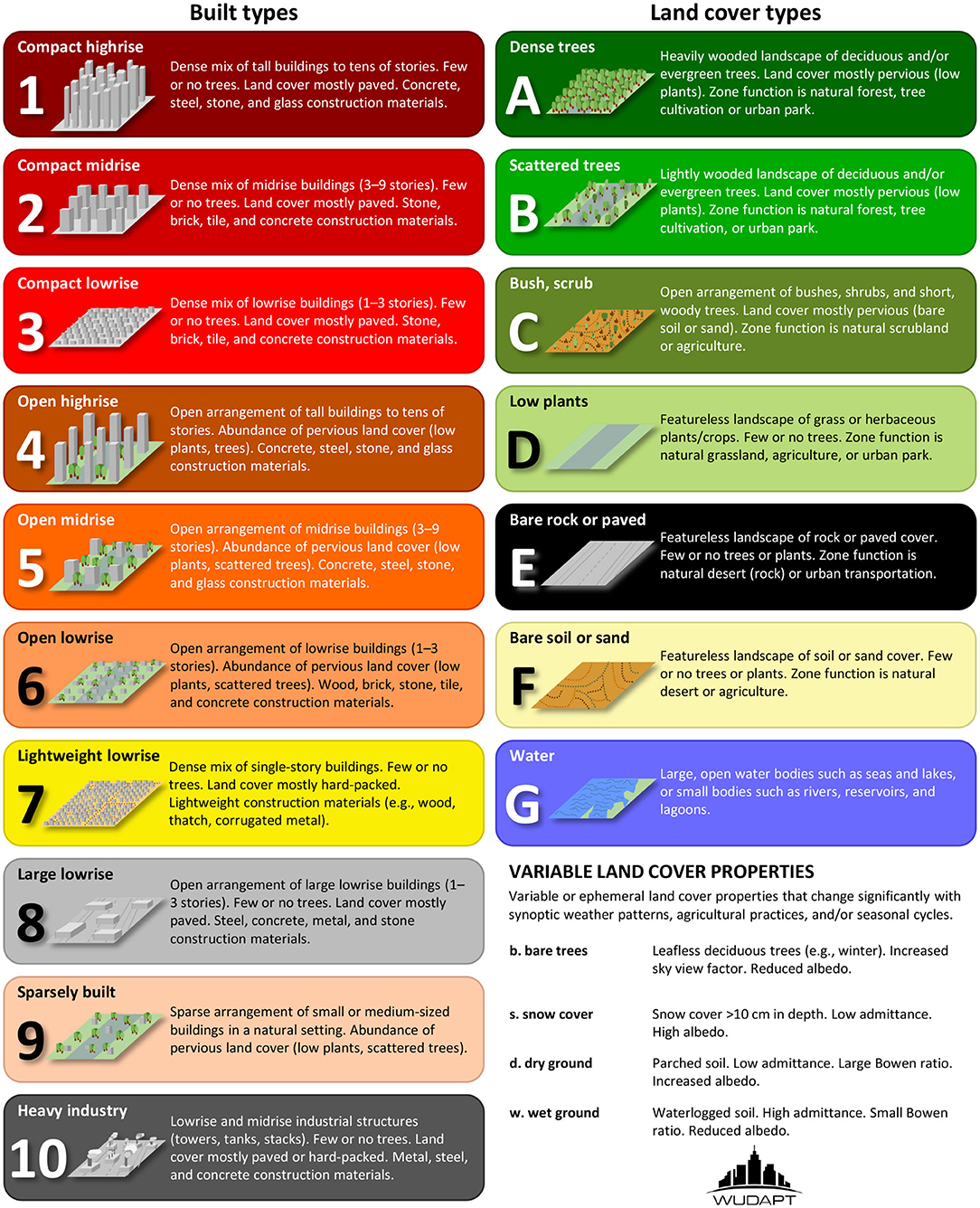
Figure 1. Urban (1–10) and natural (A–G) Local Climate Zone definitions (Stewart and Oke, 2012; Demuzere et al., 2020a).

In the early 2010s, Bechtel (2011) and Bechtel and Daneke (2012) first proposed mapping entire cities into Local Climate Zones. This procedure was formalized by Bechtel et al. (2015), relying on an “off-line” workflow that integrates training areas (TAs, a set of LCZ labeled polygons) and Landsat 8 (L8) imagery within the SAGA software package (Conrad et al., 2015) over a limited spatial domain. More specifically, each TA is identified using Google Earth images aided by the visual and numerical information provided in Stewart and Oke (2012). The TA dataset is then used to extract spectral information from L8 images, which in turn is used in a supervised random forest classifier to categorize the entire region of interest into LCZ types. This procedure was afterwards adopted by the World Urban Database and Access Portal Tools (WUDAPT) community project to create consistent LCZ maps of global cities (Ching et al., 2018).

While this framework is valuable (currently ~150 cities mapped), it will not result in a database that could support urban decision-making globally in a reasonable time frame. Therefore, Demuzere et al. (2019b,c, 2020a) developed a number of strategies to expand LCZ coverage rapidly. The first recognizes that much of the information contained in TA data for one city is transferable to other cities for which no TA data is available. The second employs Google's Earth Engine (EE)—a cloud-based platform for planetary-scale analysis (Gorelick et al., 2017)—to use its computational power, access to a range of geospatial datasets (Landsat, Sentinel, and others) and a large number of predefined algorithms. Among others, this cloud-based approach resulted in high-resolution Local Climate Zone maps for global cities, Europe and the continental United States of America (Bechtel et al., 2019a,b; Demuzere et al., 2019a,b,c, 2020a,b; Brousse et al., 2020a).

The LCZ Generator web application described here further simplifies this process, as it provides an online platform that maps a city of interest into LCZs, solely expecting a valid TA file and some metadata as input. The application integrates all of the above-mentioned developments and procedures, and simultaneously provides an automated accuracy assessment, TA data derivatives and a novel approach to identify suspicious TAs. As this contribution explains all front- and back-end procedures, databases and underlying datasets in detail, it serves as the primary “User Guide” for this web application.

2. LCZ Generator design

The LCZ Generator web application consists out of three major steps (Figure 2). In a first step, personal and training information needs to be submitted via the web application (section 2.1). Upon successful submission, the LCZ classification and quality control is launched in the back-end, to produce a quality-controlled LCZ map, metadata statistics, and labels for suspicious polygons (sections 2.2 and 2.3). In a third and final step, compressed results are sent to the user via e-mail, and simultaneously added to the online submission table (section 2.4). Each of these steps are discussed in more detail in the following sections.

FIGURE 2

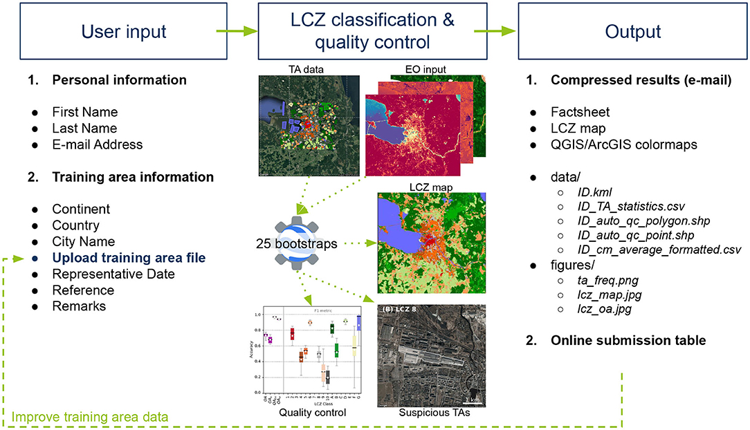
Figure 2. The LCZ Generator flowchart.

2.1. User Input

When accessing the LCZ Generator, the user is directed to a submission form that consists out of two sections: personal information and TA information (Table 1). The personal information consists out of the author's first and last name and e-mail address. The name information refers to the primary author of the TA file, which can be acknowledged in case it is used by others. The e-mail is required since the results of the LCZ Generator are sent via e-mail. If the author consents, the author's first and last name are displayed in the publicly accessible submission table and factsheet (see section 2.4).

TABLE 1

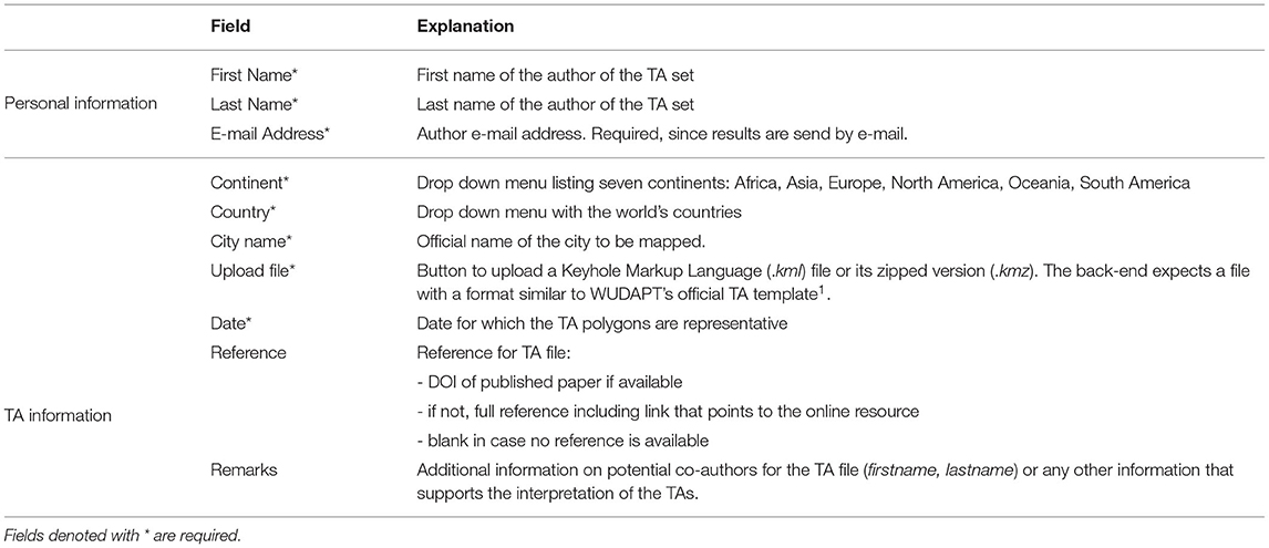
Table 1. Overview of the front-end input fields.

The second section of the submission form queries about the TA file. A user can select the continent and country via a drop-down menu, and provide the name of the city of interest. The date field refers to the date for which the training polygons are representative. This is not necessarily the date on which the TA file is created, but rather the date of the imagery (e.g., in Google Earth, see Bechtel et al., 2015) on which the labeled TAs are developed. The non-required “Reference” and “Remarks” fields allow the user to provide additional metadata about the TA file. The former can be the Digital Object Identifier (DOI) in case the TA set is published in a (peer-reviewed) paper, a reference to an online resource, or left blank if none of the previous are available. The latter allows free text and can e.g., be used to list additional authors that contributed to the creation of the TA file, or any other information that is relevant to understand the content of the TA file.

Key to the submission is the TA file itself, that can be uploaded via a button and can have any name. Yet upon submission, a file-check is done to make sure it has not been uploaded before and is compatible with the remainder of the LCZ Generator. First of all it is important that the file extension is .kml or .kmz [Keyhole Markup Language (.kml) or its zipped version (.kmz) respectively]. In case of .kmz, the file is unzipped to .kml. Second, it is checked whether the TA file can be read, and contains one or more LCZ folders, as provided in the default WUDAPT LCZ .kml template¹. This strategy is chosen as users can provide any label to a LCZ class (e.g., “LCZ 2a,” “compact midrise 1,” “not sure about this one,” …), making it difficult for the application to assign an appropriate LCZ label required for the classification. If folders are available, the folder names are used to rename their underlying polygons. Third, if present, empty polygons are removed (e.g., “Style Place Holders” that were not deleted from the .kml template). Fourth, each polygon is provided with a unique ID, which is required to perform the automated TA quality control (see section 2.3). Finally, also the size of the region of interest (ROI) is checked. The ROI is defined as the outer extent of the TA polygons, currently with an additional buffer on all sides of 10 km. In order to maintain computational efficiency, the maximum allowed ROI size is currently set to 2.5° x 2.5°.

If any of the above checks fail, a red-framed message is returned to the user upon submission, instructing about ways to solve the issue. If all tests pass, a green-framed message is returned, and the LCZ Generator is launched in the back-end.

2.2. LCZ Classification and Quality Control

Before the TAs are used in the classification procedure, they undergo a final pre-processing step: the surface area of large polygons (>1.5 km²) is reduced to a radius of approximately 350 m, in line with Demuzere et al. (2019b,c, 2020a) and the minimum allowed surface area described in section 2.3. These large polygons typically represent homogeneous areas such as water bodies and forests, a characteristic that is neither needed nor wanted, as it leads to more imbalanced TA data and computational inefficiency of the classifier.

In addition to the TAs, one needs earth observation data and a supervised classifier (Bechtel et al., 2015). The default WUDAPT workflow relies on Landsat 8 data as input to the random forest classifier, embedded as an “LCZ classification tool” in SAGA GIS (Breiman, 2001; Bechtel et al., 2015; Conrad et al., 2015). Yet here, the LCZ Generator builds further upon the findings of Demuzere et al. (2019b,c, 2020a), Brousse et al. (2020a), in which additional earth observations are used, in combination with the TAs, as input to EE's implementation of the random forest classifier.

Currently, a total of 33 input features are available globally, on a 100 m resolution, and are stored in EE's online WUDAPT asset folder (3 TB of data) (Table 2). They consist out of 16 features derived from Landsat 8, 5 features from Sentinel-1, 8 features from Sentinel-2, and four additional features reflecting terrain and forest canopy height. Note that the list of input features used in Demuzere et al. (2019b, 2020a) is expanded with Sentinel-2 red edge bands to improve the mapping of wetlands (Forkuor et al., 2018; Kaplan and Avdan, 2018; Brousse et al., 2020a), and a Sentinel-2-based combinational shadow index (CSI) and shadow enhancement index (SEI) median composite (Sun et al., 2019). The system is designed in such a way that, whenever additional, new or improved global earth observation datasets become available, they can easily be added to the asset folder and activated in the classification procedure.

TABLE 2

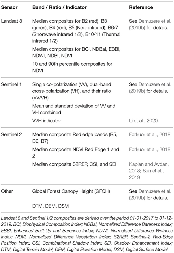
Table 2. Earth observation input features currently available for the LCZ Generator.

To ensure the quality of the resulting LCZ map, quality control is a vital step (Verdonck et al., 2017). Hence, an automated cross-validation approach using 25 bootstraps is applied (Bechtel et al., 2019a). In each bootstrap, 70% of the TA polygons are used to train and 30% to test; the polygons are selected by stratified (LCZ type) random sampling, maintaining the original LCZ class frequency distribution. This procedure is repeated 25 times allowing us to provide confidence intervals around the accuracy metrics. In addition, this approach also allows the creation of a probability map, which indicates how often (in %) the mode was mapped in the iterative procedure.

The resulting LCZ map provided to the user is based on all TAs (100% of the TA polygons) and input features. A filtered version is also provided using the morphological Gaussian filter described in more detail in Demuzere et al. (2020a). This is preferred over the WUDAPT's traditional majority post-classification, as it accounts for the distance from the center of the kernel and differences in the typical patch size between classes. For example, linear features like rivers are typically removed by the majority filter. The LCZ map, its Gaussian-filtered version and the probability map are provided to the user as a single .tif with three bands: “lcz,” “lczFilter,” and “classProbability,” respectively.

The accuracy metrics used follow previous work (see Demuzere et al., 2020a, and references therein): overall accuracy (OA), overall accuracy for the urban LCZ classes only (OA_u), overall accuracy of the built vs. natural LCZ classes only (OA_bu), a weighted accuracy (OA_w), and the class-wise metric F1. The overall accuracy denotes the percentage of correctly classified pixels. OA_u reflects the percentage of classified pixels from the urban LCZ classes only, and OA_bu is the overall accuracy of the built vs. natural LCZ classes only, ignoring their internal differentiation. The weighted accuracy (OA_w) is obtained by applying weights to the confusion matrix and accounts for the (dis)similarity between LCZ types (Bechtel et al., 2017, 2020). For example, LCZ 4 is most similar to the other open urban types (LCZs 5 and 6), leaving these pairs with higher weights compared to e.g., an urban and natural LCZ class pair. This results in penalizing confusion between dissimilar types more than confusion between similar classes. Finally, the class-wise accuracy is evaluated using the F1 metric, which is a harmonic mean of the user's and producer's accuracy (Verdonck et al., 2017). Accuracy results are provided to the user in two ways: average confusion matrix over the 25 bootstraps (_cm_average_formatted.csv), including Overall, User and Producer Accuracy (in %) and a boxplot figure (_cm_oa_boxplot.jpg) depicting the range of all accuracy metrics over all bootstraps.

2.3. Automated TA Quality Control

Sections 2.1 and 2.2 are at the core of the LCZ Generator application, explaining how a user's TA dataset combined with a wealth of earth observation input feeds the random forest classifier, resulting in a quality-controlled LCZ map. Yet an additional automated 3-step TA quality control is added, that aims to facilitate the revision of the original TA submission and resulting LCZ map, since previous work by Bechtel et al. (2017, 2019a) and Verdonck et al. (2019) highlighted that multiple iterations can significantly improve the overall accuracy of the LCZ map, and are thus recommended.

Stewart and Oke (2012) suggested that the typical horizontal scale of a Local Climate Zone—reflecting an area of uniform surface cover, structure, and material—spans hundreds of meters to several kilometers. In addition, the number of TAs selected for each zone can be an indicator for zones which are hard to classify, and the WUDAPT protocol suggests to digitize compact and simple TA sets, characterized by a shape ratio close to one (Bechtel et al., 2019a; Verdonck et al., 2019). Therefore, a summary table (_TA_statistics.csv) is added to the output, providing, for each available LCZ class, the number of polygons (Count, C), the average and total surface area (Avg. / Total area, km²), the perimeter (km), the shape (-), and number of vertices (-).

Subsequently, a 3-step automated quality control (QC) is applied to label suspicious TA polygons. In a first step (qc_step1), polygons with a surface area below 0.04 km² (too small) or a shape ratio 3 (too complex shape) are flagged. In a second step (qc_step2), the non-parametric density-based spatial clustering of applications with noise (DBSCAN) (Ester et al., 1996; Schubert et al., 2017) is used to identify whether the average spectral value of a polygon of LCZ class i is considered as an outlier compared to the average spectral values of all other polygons of that class i. The method requires two parameters: ϵ, which is the maximum distance between two samples for one to be considered as in the neighborhood of the other, and MinPoints, the number of minimum samples in a neighborhood for a point to be considered as a core point. Here, ϵ is set to 0.3 and MinPoints to C_i/10, based on a number of iterations and expert judgement. Since this method is efficient on large, multi-dimensional datasets, it is applied simultaneously on all earth observation input features discussed in section 2.2.

A third and final QC step (qc_step3) considers all individual pixel values of all polygons in each LCZ class i compared to the polygon average approach from qc_step2. The same parameter values for ϵ and MinPoints are used, and the procedure is also applied on all available input features simultaneously. The pixel's latitude and longitude coordinates here serve as an unique identifier to tag suspicious points within polygons.

If polygons are identified as suspicious, the user receives two shapefiles containing the results of the automated quality control procedure. The first shapefile (ID_auto_qc_polygon.shp) contains all polygons flagged as suspicious in at least one of the tree steps. Since qc_step3 returns points, each polygon that intersects with at least one of these flagged points is added. All shapes in this file contain additional metadata fields characterizing their geometry (area, perimeter, shape, vertices) and a boolean value for each of the three QC steps: True (1) / False (0) in case a TA passed / failed one of the three QC tests. The second shapefile (ID_auto_qc_point.shp) contains the individual flagged points, which might provide additional insights into why certain polygons are flagged as suspicious. In case no polygons or points are labeled as suspicious, the same files are created yet only contain a point with a dummy identifier and a geometry indicating the center pixel of the ROI.

2.4. Generated Output

If the LCZ Generator successfully completes all processes, the user is notified via e-mail, that contains a compressed (.zip) archive as attachment. This archive (Table 3) contains the various outputs described in sections 2.2 and 2.3.

TABLE 3

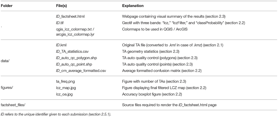
Table 3. File structure and contents of the compressed (.zip) results send to the user via e-mail.

The output is listed in an online search- and sortable submission table including information about the city, country, continent, date of the submission, overall accuracy, and a button (Show Factsheet) linking to the factsheet that provides a visual summary of all results. In case a user did not agree to display his/her name (see section 2.1), the Author field is left blank in both the submission table and factsheet. By checking one or multiple entries using the left-hand side check-boxes of the submission table, one can also download the corresponding .zip archive(s).

The submission table is structured as follows. If a user submitted multiple TAs for one city, only the submission having the best overall accuracy is displayed. In case multiple users submit TAs for the same city, only the best result is displayed, but this time for each individual user. A button (Show all submissions) allows the user to view and download all submissions including those where one author submitted multiple versions of TAs for the same city. This structure ensures that only results with the best possible quality are directly available for download, but also that this web application can be used for learning purposes and improving the TA creation technique without adding multiple previous submissions of minor quality to the table.

In the event the LCZ Generator fails after successfully submitting the TAs, the user is notified via e-mail as well. In this case, the developers automatically receive a message, and can use the log stored in the back-end to solve the issue.

2.5. Technical Information, Terms of Service, and Attribution Guidelines

2.5.1. Database

All data including the author and submission information, as well as the processing outputs are stored with a unique ID in a PostgreSQL database. The TAs are stored in a PostGIS table as individual polygons.

2.5.2. Versioning

The LCZ-Generator code will be versioned according to semantic versioning²: breaking changes to the application programming interface (API)—including changes to the input features (Table 2)—will be indicated by an incremented major version. After the release of version 1.0.0, and for each next release, all changes will be described in a changelog, available on the issue page (section 2.5.3). The version used for creating each LCZ map is stored for each submission and included in the corresponding factsheet.

2.5.3. Support

Guidance in how to use the LCZ Generator is provided via the “Getting started” and “Frequently Asked Questions (FAQ)” pages, accessible via the navigation bar of the web application. If users run into issues while using the LCZ Generator, they can open a public issue on the application's Github issue tracker³. In case security bugs are found, we ask the user to not create a public issue but instead reach out to us directly via lcz-generator@rub.de.

2.5.4. Terms of Service and Attribution Guidelines

The web application uses the CC BY-SA 4.0 license⁴ for all submissions made. The terms of service⁵ need to be accepted upon submission. In addition, attribution guidelines⁶ are provided on how to acknowledge the materials produced by the LCZ Generator, the authors of the TAs or any of the underlying methods used in the Generator's classification procedures. This information is also embedded at the end of the factsheet (see also section 3.1).

2.6. Test Samples

In this paper, the performance of the LCZ Generator web application is demonstrated via three new TA samples, compiled by three student assistants at the Ruhr University Bochum (Germany). The samples are from different urban ecoregions—which stratify urban areas based on general climate and vegetation characteristics, regional differences in urban topology, and the level of economic development (Schneider et al., 2010)—and include Saint Petersburg (Russia, “Temperate forest in Asia”), Bamako (Mali, “Tropical, sub-tropical Savannah in Africa”), and Havana (Cuba, “Tropical broadleaf forest in South America”). The TAs are a first version, and did not undergo a manual review by an experienced operator (Bechtel et al., 2019a).

3. Results

This section presents and discusses all contents of the resulting .zip archive in more detail. Note that all LCZ results in this paper are displayed with labels 1–10 for the urban classes, and A to G for the natural classes, in line with Stewart and Oke (2012) (Figure 1). However, all underlying files output by the LCZ generator use integers, with labels 11 to 17 for the natural classes.

3.1. Submission Table

Figure 3 provides a factsheet example for the city of Saint Petersburg. It summarizes author, submission, TA and LCZ map & accuracy information. In addition to the author's input discussed in section 2.1, the submission information also contains the submission date, the software version, and the ID. The software version tag is linked to the software's version in GitHub, so that at any point in time it is clear with which code and parameters each submission is produced (section 2.5.2). The TA information section lists the content of the ID_TA_statistics.csv, that is also linked. In addition, a figure is added that displays the number of TAs per available LCZ class. This figure is stored as ta_freq.png. Finally, the LCZ map & accuracy section provides quick access to all four overall accuracy scores, together with an image of the actual filtered LCZ map (stored as lcz_map.jpg). Hyperlinks to all underlying data files are provided as well, e.g., by clicking the “boxplot figure with accuracies” link, the author can directly see the full accuracy assessment, including information from all bootstraps and class-wise F1 scores.

FIGURE 3

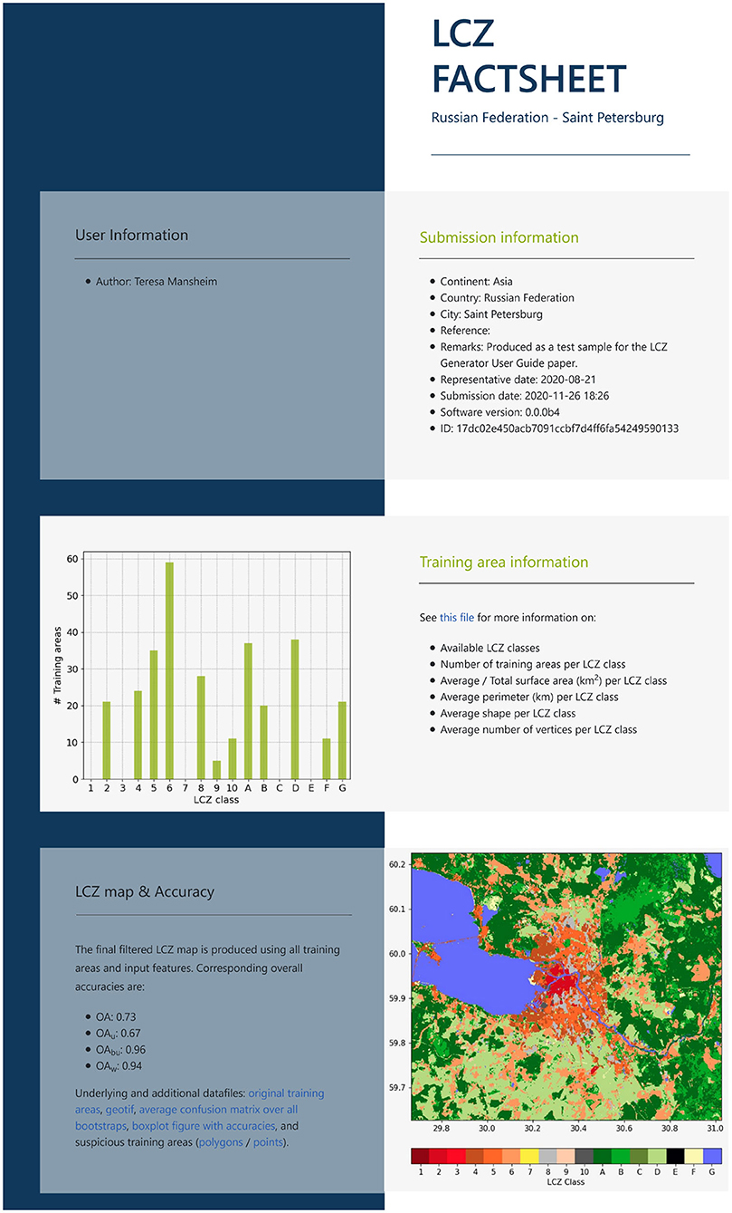
Figure 3. Factsheet example for Saint Petersburg. Note that in reality, the factsheet also contains a “Terms of Service” and “Attribution” section (see section 2.5.4). These sections are omitted here for clarity.

3.2. LCZ Map and Accuracies

Feeding the random forest in a bootstrapping manner with the submitted TAs (Figure 4) and the earth observation input features (Table 2) results in a raw and filtered LCZ map, a pixel probability map (Figure 5) and overall accuracy metrics (Figure 6). Combined with the information from the factsheet (Figure 3) and the ID_TA_statistics.csv file, one can directly assess the amount and distribution of TA polygons. For Saint Petersburg, a total of 310 TA polygons are available, with the highest / lowest frequencies for LCZ 6 (Open lowrise) and 14 (Low plants) / LCZ 9 (Sparsely built) and 10 (Heavy industry).

FIGURE 4

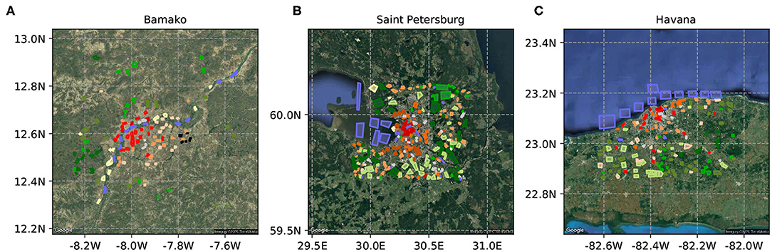
Figure 4. Training areas for (A) Bamako, (B) Saint Petersburg, and (C) Havana. Color scheme as in Figure 1.

FIGURE 5

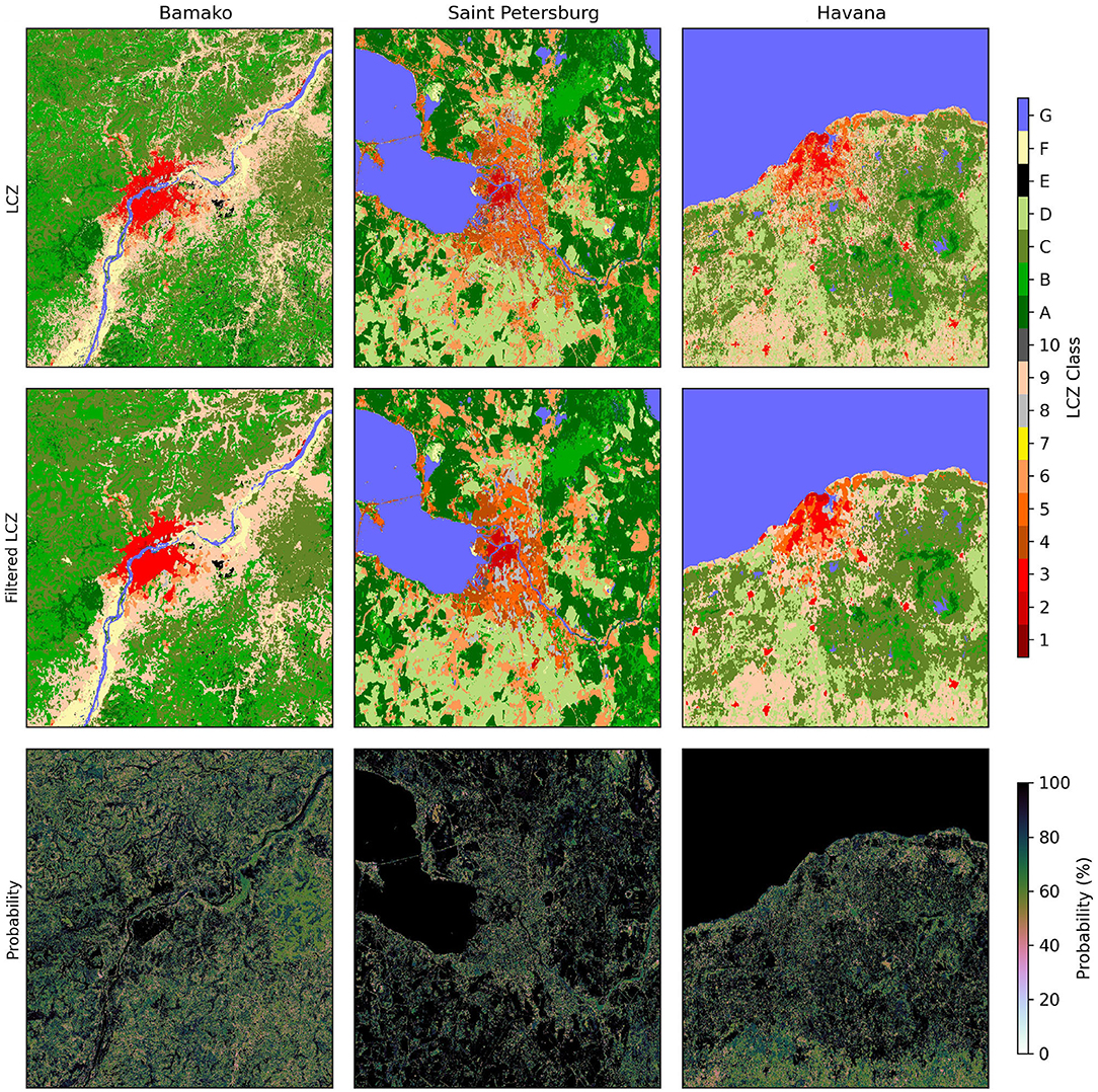
Figure 5. Information contained in the geotif output file, for all cities (columns): final LCZ map (Top), final filtered LCZ map (Middle), and probability map (Lower).

FIGURE 6

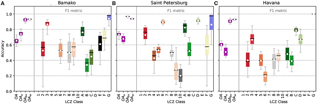
Figure 6. Accuracies for (A) Bamako, (B) Saint Petersburg, and (C) Havana. The purple colors in the box plots refer to the overall accuracy metrics, while the LCZ colored boxes reflect the class-wise F1 metric. Mean and median are depicted by a white dot and black line respectively, boxes indicate the interquartile range and whiskers the 5 to 95th quartile range.

The raw and filtered LCZ maps (Figure 5) differ mainly in their fine-scale heterogeneity: as single pixels do not constitute an LCZ class, the Gaussian filter procedure is able to remove this granularity. Since the Gaussian parameters (standard deviation and kernel size) are currently derived by experts, and expected to differ between cities and continents (Demuzere et al., 2020a), they deserve further attention and potential adjustments in future versions of the LCZ Generator. The probability maps in Figure 5 indicate how often (in %) the mode LCZ class was mapped during the bootstrapping procedure. In general, areas covered by TAs are often mapped as the same LCZ class more than 80% of the time (>20/25 iterations). Areas at the boundaries of the ROI, e.g., southern edge of the Havana domain, or east of Bamako, are often characterized by lower probability scores. Such information helps authors to identify where confusion exists in their ROI.

Finally, the accuracy of the lcz map can be assessed using the accuracy metrics discussed in section 2.2 and displayed in Figure 6. For all three cities, the average overall accuracy metrics reach values above 0.5, a minimum accuracy level proposed by Bechtel et al. (2019a) to pass the automated quality control. Lowest class-wise F1 metrics can be seen for LCZs 9 and 10 in Saint Petersburg (corresponding to the LCZs with the lowest TA polygon frequencies), and LCZ 6 in Havana. Note that no F1 metric is available for LCZ 7 in Bamako, even though one TA polygon is available in the TA set (Figure 4A). This is because a single polygon does not suffice to perform a quality assessment due to the stratified random sampling of the TAs in training and test data. This is in line with the results of the HUMan INfluence EXperiment (HUMINEX, Bechtel et al., 2017; Verdonck et al., 2019) indicating that, when the number of TAs for a specific zone is low, the representativeness of this TA might be low, leading to lower accuracies. This is often caused by (inexperienced) authors spending a lot of time searching for TAs for all seventeen LCZs, even though some of the zones are not large enough or occur too sparsely in the city to constitute a LCZ.

3.3. Automated TA Quality Control

In total, 36 (25%), 80 (25%), and 27 (16%) polygons are flagged as suspicious in at least one of the quality control steps, for Bamako, Saint Petersburg, and Havana, respectively. Some examples from all cities and for each quality control step are described in more detail below.

Figure 7 displays all polygons from Saint Petersburg flagged as suspicious during the first quality control step. Two polygons are flagged because they have a surface area below the 0.04 km² threshold (Figures 7C,H), the remainder because of their shape exceeding the maximum allowed value of 3. The latter polygons typically correspond to linear (narrow and very long) shapes, often pointing to rivers (LCZ 17, Figures 7E,G,I) or complex shapes not adhering to the guidelines of digitizing simple block shapes (Figures 7A,B). While these are not necessarily wrong, complex shapes may lead to a suboptimal sampling of the satellite input features, or may lead to a mixed spectral signature in case polygons are too narrow and/or are close to other land covers/uses (Verdonck et al., 2019). More information on best practices for digitizing TAs is available in Verdonck et al. (2019) and on the WUDAPT webpage⁷.

FIGURE 7

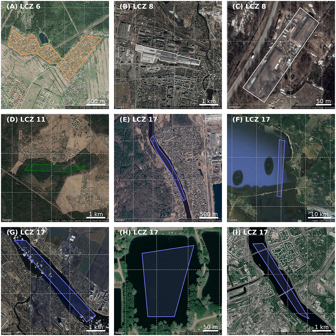
Figure 7. All TA polygons tagged as suspicious during the first quality control step, for Saint Petersburg. Color scheme as in Figure 1.

Some examples for the second quality control step are shown in Figure 8. They are all natural LCZ classes consisting out of LCZ 11 (or A, Dense trees), 12 (or B, Scattered trees), 16 (or F, Bare soil or sand) and 17 (or G, Water). The true color RGB satellite information reveals that the dense tree polygon (Figure 8A) might be closer to LCZ B (Scattered trees). This is supported by the spectral profiles in Figure 9A, with e.g., lower values for the forest canopy height (GFCH), and higher values for Landsat's red (L8_B4) and thermal infrared (L8_B10/B11) bands, when compared to the expected spectral value space for all LCZ 11 polygons. For the LCZ 12 polygons (Figures 8B,C), the true color satellite imagery reveals a rather heterogeneous landscape, covered by patches of dense and scattered trees, agricultural fields, bare soils, small settlements or sparsely built areas, and a small (seasonal) river. The latter two are captured by the higher than expected value for Landsat's NDWI (L8_NDWI) and a lower than expected enhanced built up and bare soil index (L8_EBBI), where lower EBBI values refer to built-up areas (As-syakur et al., 2012) (Figure 9B). The polygon in Figure 8D is labeled as bare soil or sand, even though the man-made land use pattern suggest this area to be farm land, which should thus be labeled as LCZ 14 (or D, Low plants). This is also visible from Landsat's median, 10 and 90th percentile normalized difference vegetation index values (L8_NDVI(_P10/_P90) being higher than the expected LCZ 16 values (Figure 9C). Lastly, the LCZ 17 polygons in Figures 9E,F represent two sections of the Niger river, characterized by strong fluctuations in water levels according to the rainy and dry seasons. Using the Global Surface Water Explorer⁸ (Pekel et al., 2016) or Google's timelapse tool⁹, one can infer that these polygons are mapped in sections of the river that are seasonal and thus only have water for some time of the year. This is supported by the Landsat's NDVI and NDWI values for the LCZ 17 polygons (Figures 9D, 10): while all LCZ 17 polygons are sampling from the Niger river (Figure 4A), the NDWI values for the polygons in Figures 8E,F are significantly lower than those from the other polygons. The same but opposite observation can be made for the NDVI values.

FIGURE 8

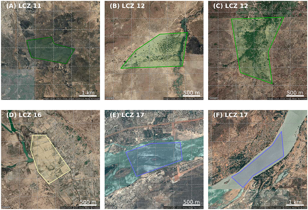
Figure 8. A selection of TA polygons tagged as suspicious during the second quality control step, for Bamako. Color scheme as in Figure 1.

FIGURE 9

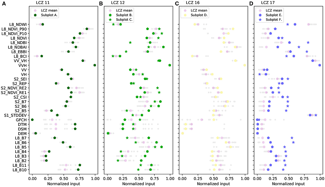
Figure 9. Normalized polygon-averaged spectral input values (gray dots), for all LCZ classes shown in Figure 8, for Bamako. Pink circles denote the mean over all polygons, other markers in corresponding LCZ colors refer to the polygons shown in Figure 8.

FIGURE 10

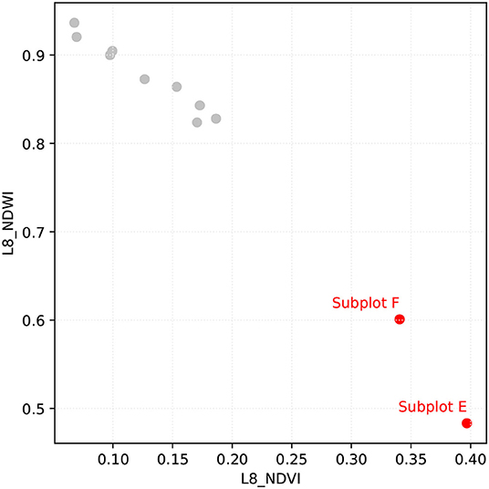
Figure 10. Average Landsat's NDVI and NDWI values for all LCZ 17 polygons, for Bamako. Suspicious polygons from subplots E and F in Figure 8 are shown in red.

The third quality control step performs a similar analysis as the second step, yet this time on the pixel level. Figure 11 displays a selected number of polygons over Havana, together with the pixels flagged as suspicious. The first polygon (Figure 11A) is labeled as LCZ 9 (Sparsely built), reflecting the small or medium-sized buildings widely spaced across a landscape with abundant vegetation. Yet the polygon also includes a water body large enough to be detected by the 100 m input feature pixels. Visualizing the NDWI values of these pixels against e.g., the combined shadow index derived from Sentinel-2 (S2_CSI) reveals the outlier position of these pixels (Figure 12A). A similar analysis can be done for the other selected polygons: the LCZ 14 polygon in Figure 11B mostly constitutes agricultural land, yet also contains a farm flagged as suspicious. The compact lowrise LCZ 3 polygon in Figure 11C contains a park in the middle surrounded by trees, being flagged as suspicious. Figure 11D is labeled as LCZ 13 (Bush and scrub) even though it should probably be LCZ D (Low plants). The flagged dots in this case refer to areas with seasonal waters, which can again be visualized using Google Earth's historical imagery tool. Finally, Figures 11E,F are two additional examples of compact lowrise polygons. And even though some of the spectral signatures tend to be outliers compared to all other pixel values for this LCZ class (Figures 12E,F), it is not self-evident to pin-point the exact reasons for the polygons to be flagged. In Figure 11E, a pixel is flagged with abundant vegetation, yet elsewhere in the polygon similar areas can be found that are not flagged. The polygon in Figure 11F represents a homogeneous neighborhood in terms of urban form, yet here the flagged pixel is on top of a large-scale warehouse, potentially large enough to influence the pixel's spectral values with its different radiative characteristics.

FIGURE 11

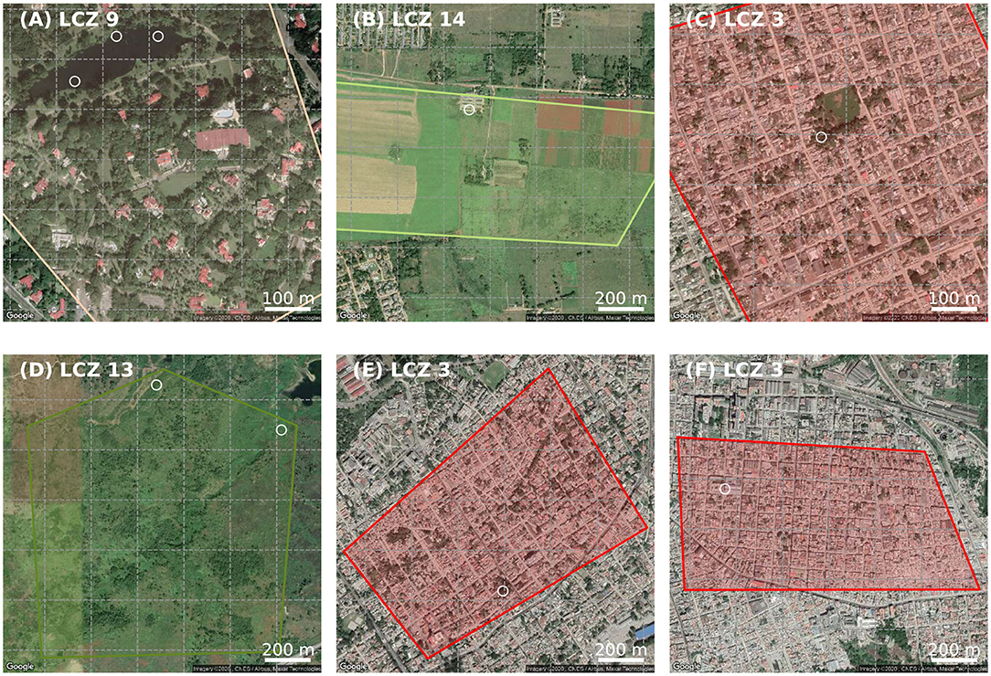
Figure 11. As Figure 8, but for the third quality control step, for Havana. White circles refer to the centroids of the actual pixels flagged in this quality control step.

FIGURE 12

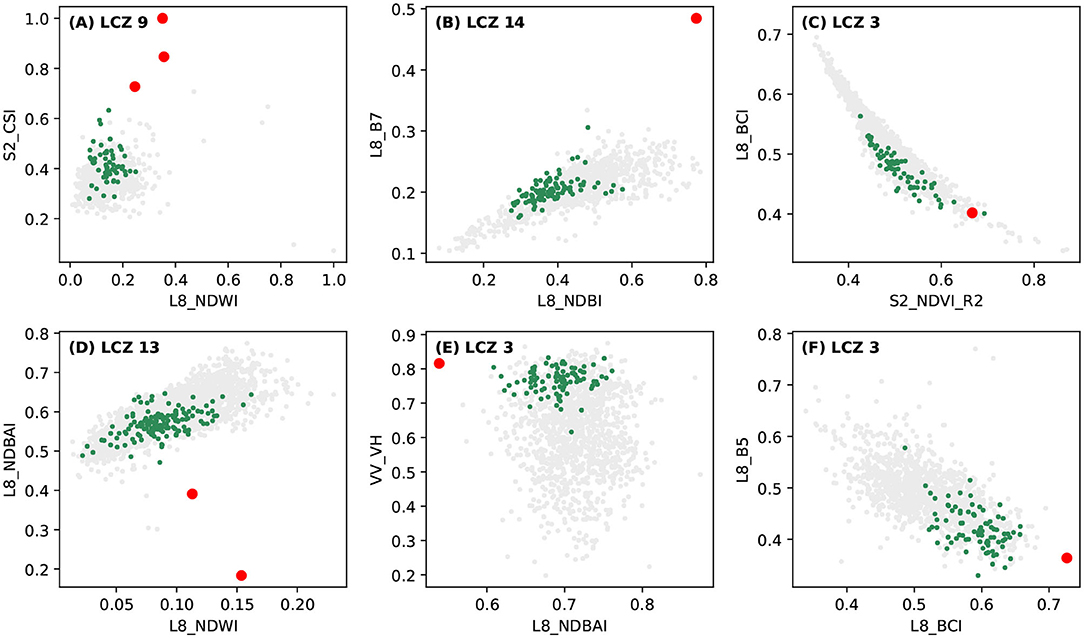
Figure 12. Spectral values for all pixels in one LCZ class, corresponding to the subplots of Figure 11 (gray dots). Pixels flagged as outliers by DBSCAN are shown in red. Remaining pixels from the pixel's parent polygon are shown in green.

4. Discussion and conclusions

Since their introduction in 2012 (Stewart and Oke, 2012), Local Climate Zones (LCZs) emerged as a new standard for characterizing urban landscapes, providing a holistic classification approach that takes into account micro-scale land-cover and associated physical properties (Demuzere et al., 2020a). This is reflected by the growing number of scientific publications having “LCZ” or “Local Climate Zones” listed as keywords: according to Web of Science, as of February 4 2021, a total of 139 papers were published, 38 of them in 2020 alone. The default LCZ mapping procedure, adopted as Level 0 (lowest level of detail) by the WUDAPT grass-root effort, and relying only on open-source data (Landsat 8) and software (SAGA GIS, Conrad et al., 2015), was certainly instrumental to this success (Bechtel et al., 2015; Ching et al., 2018). However, some features of this default procedure inhibit global up-scaling in a reasonable time, e.g., the need to download and pre-process Landsat 8 data from the United States Geological Survey (USGS) Earth Explorer, the processing of the LCZ classifier embedded in SAGA GIS on your local computer, the unavailability of an automated cross-validation, and the manual review by an experienced operator before the data is made publicly available (Bechtel et al., 2015, 2019a).

The LCZ Generator addresses these shortcomings, by adopting well-tested and -documented cloud-based LCZ mapping strategies using Google's earth engine (Gorelick et al., 2017; Brousse et al., 2019, 2020a,b; Demuzere et al., 2019b,c, 2020a,c; Varentsov et al., 2020). The result of this is an online platform, that maps a city of interest into LCZs, solely expecting a valid TA file and some metadata as input. The web application simultaneously provides an automated accuracy assessment, in line with the cross-validation procedure detailed in Bechtel et al. (2019a). To date, this bootstrap-based accuracy assessment was not available in the SAGA GIS context, often leading to insufficiently robust accuracy assessments during the production of LCZ maps (Verdonck et al., 2017). In addition, the novel 3-step TA quality control facilitates the revision of the original TAs, allowing the user to revise the initial submission, and re-submit to the LCZ Generator, as previous work highlighted the importance of additional iterations (Bechtel et al., 2017, 2019a; Verdonck et al., 2019). Results in this study reveal for example that users should be more careful when digitizing TAs (e.g., compact shapes, scales, and borders), and should take into account seasonal properties of the underlying land cover/use. Note however that this TA quality control implementation is still experimental, and was successfully tested on a limited number of TA samples only. The LCZ Generator can assist in this respect to gather more TA samples in order to populate a spectral LCZ library across urban (eco)regions (Jackson et al., 2010; Schneider et al., 2010; Demuzere et al., 2019c), enabling a better assessment of spectral outliers.

The LCZ Generator should be considered as a dynamic application, that will be updated whenever new scalable mapping techniques and globally-available input features become available. In case updates occur in the future, they will be tracked via the software version number and described in the changelog available on the Github Issue page. For example, some successfully tested the use of object-based image analysis (Collins and Dronova, 2019; Simanjuntak et al., 2019), others obtained promising results using (residual) convolutional neural networks (Qiu et al., 2019, 2020; Yoo et al., 2019; Liu and Shi, 2020; Rosentreter et al., 2020; Zhu et al., 2020). Yet to date, the feasibility of such procedures for large-scale LCZ mapping has not yet been demonstrated (Demuzere et al., 2020a). Many others have developed GIS-based approaches using datasets from e.g., city administrations or derived from crowd-sourced cartographic services such as OpenStreetMap (Lelovics et al., 2014; Quan et al., 2017; Samsonov and Trigub, 2017; Wang et al., 2018; Hidalgo et al., 2019; Quan, 2019; Oliveira et al., 2020; Zhou et al., 2020). The latter study also proposes an extension to the default WUDAPT accuracy assessment, by integrating GIS data (e.g., building footprints and heights, and pervious surface fraction). While all these efforts are considered valuable, they have one thing in common limiting their implementation into the LCZ Generator: the underlying datasets are to date not globally available.

We anticipate that the LCZ Generator will ease the production, quality assessment and dissemination of LCZ maps and related products. This easy-to-use and accessible online platform should therefore continue to support researchers and practitioners in using the LCZ framework for a variety of applications, such as urban heat (risk) assessment studies (Demuzere et al., 2020a, and references therein), climate sensitive design and urban planning (policies) (Perera and Emmanuel, 2016; Vandamme et al., 2019; Maharoof et al., 2020), anthropogenic heat and building carbon emissions (Wu et al., 2018; Santos et al., 2020), quality of life (Sapena et al., 2021), multi-temporal urban land change (Vandamme et al., 2019; Wang et al., 2019), and urban health issues (Brousse et al., 2019, 2020a). This development will in addition accelerate the key aim of WUDAPT, that is “to capture consistent information on urban form and function for cities worldwide that can support urban weather, climate, hydrology and air quality modeling” (Ching et al., 2018, 2019). Examples of modeling systems currently using LCZ information are the Surface Urban Energy and Water Balance Scheme (SUEWS, Alexander et al., 2016), ENVI-met (Bande et al., 2020), the urban multi-scale environmental predictor (UMEP, Lindberg et al., 2018), MUKLIMO_3 (Bokwa et al., 2019; Gál et al., 2021), COSMO-CLM and the WUDAPT-TO-COSMO tool (Wouters et al., 2016; Brousse et al., 2019, 2020b; Varentsov et al., 2020), and the Weather Research and Forecasting model (WRF, Brousse et al., 2016; Hammerberg et al., 2018; Wong et al., 2019; Patel et al., 2020; Zonato et al., 2020). While WRF currently uses the WUDAPT-to-WRF tool to ingest LCZ information (Brousse et al., 2016), its next release expected in spring 2021 should offer this compatibility by default (A. Zonato, personal communication).

To conclude, and in line with the assessment of Creutzig et al. (2019), we firmly believe that this LCZ Generator has the potential to become a key part in mainstreaming and harmonizing urban data collection, upscale urban climate solutions and effect change at the global scale.

Data Availability Statement

Publicly available datasets were analyzed in this study. This data can be found at: https://lcz-generator.rub.de.

Author Contributions

The authors jointly devised the concept of the LCZ Generator. MD developed the LCZ-related codes. JK developed the database and front- and back-end. MD developed all visualizations. MD led the writing with contributions from JK and BB.

Funding

This work was conducted in the context of project ENLIGHT, funded by the German Research Foundation (DFG) under grant No. 437467569.

Conflict of Interest

The authors declare that the research was conducted in the absence of any commercial or financial relationships that could be construed as a potential conflict of interest.

Acknowledgments

We thank USGS and NASA for the free Landsat data, and the Copernicus programme of ESA for the Sentinel data, all acquired and processed via Google's earth engine. We acknowledge support by the Open Access Publication Funds of the Ruhr-Universität Bochum (RUB, Germany). Moreover, we thank RUB's student assistants Christian Moede, Lara van der Linden, and Teresa Mansheim for the training areas used in this study.

Footnotes

1. ^http://www.wudapt.org/wp-content/uploads/2020/08/WUDAPT_L0_Training_template.kml

2. ^https://semver.org/

3. ^https://github.com/RUBclim/LCZ-Generator-Issues

4. ^https://creativecommons.org/licenses/by-sa/4.0/

5. ^https://lcz-generator.rub.de/tos

6. ^https://lcz-generator.rub.de/attribution

7. ^http://www.wudapt.org/create-lcz-training-areas/

8. ^https://global-surface-water.appspot.com/map

9. ^https://earthengine.google.com/timelapse/

References

Alexander, P., Bechtel, B., Chow, W., Fealy, R., and Mills, G. (2016). Linking urban climate classification with an urban energy and water budget model: multi-site and multi-seasonal evaluation. Urban Clim. 17, 196–215. doi: 10.1016/j.uclim.2016.08.003

CrossRef Full Text | Google Scholar

As-syakur, A. R., Adnyana, I. W. S., Arthana, I. W., and Nuarsa, I. W. (2012). Enhanced built-UP and bareness index (EBBI) for mapping built-UP and bare land in an urban area. Remote Sens. 4, 2957–2970. doi: 10.3390/rs4102957

CrossRef Full Text | Google Scholar

Bai, X., Dawson, R. J., Ürge-Vorsatz, D., Delgado, G. C., Barau, A. S., Dhakal, S., et al. (2018). Six research priorities for cities. Nature 555, 23–25. doi: 10.1038/d41586-018-02409-z

CrossRef Full Text | Google Scholar

Baklanov, A., Grimmond, C., Carlson, D., Terblanche, D., Tang, X., Bouchet, V., et al. (2018). From urban meteorology, climate and environment research to integrated city services. Urban Clim. 23, 330–341. doi: 10.1016/j.uclim.2017.05.004

CrossRef Full Text | Google Scholar

Bande, L., Manandhar, P., Ghazal, R., and Marpu, P. (2020). Characterization of local climate zones using ENVI-met and site data in the city of Al-Ain, UAE. Int. J. Sustain. Dev. Plann. 15, 751–760. doi: 10.18280/ijsdp.150517

CrossRef Full Text | Google Scholar

Bechtel, B. (2011). “Multitemporal Landsat data for urban heat island assessment and classification of local climate zones,” in 2011 Joint Urban Remote Sensing Event (Munich: IEEE), 129–132.

Google Scholar

Bechtel, B., Alexander, P., Böhner, J., Ching, J., Conrad, O., Feddema, J., et al. (2015). Mapping local climate zones for a worldwide database of the form and function of cities. ISPRS Int. J. Geo Inform. 4, 199–219. doi: 10.3390/ijgi4010199

CrossRef Full Text | Google Scholar

Bechtel, B., Alexander, P. J., Beck, C., Böhner, J., Brousse, O., Ching, J., et al. (2019a). Generating WUDAPT Level 0 data – Current status of production and evaluation. Urban Clim. 27, 24–45. doi: 10.1016/j.uclim.2018.10.001

CrossRef Full Text | Google Scholar

Bechtel, B., and Daneke, C. (2012). Classification of local climate zones based on multiple earth observation data. IEEE J. Sel. Top. Appl. Earth Observ. Remote Sens. 5, 1191–1202. doi: 10.1109/JSTARS.2012.2189873

CrossRef Full Text | Google Scholar

Bechtel, B., Demuzere, M., Mills, G., Zhan, W., Sismanidis, P., Small, C., et al. (2019b). SUHI analysis using Local Climate Zones—A comparison of 50 cities. Urban Clim. 28:100451. doi: 10.1016/j.uclim.2019.01.005

CrossRef Full Text | Google Scholar

Bechtel, B., Demuzere, M., Sismanidis, P., Fenner, D., Brousse, O., Beck, C., et al. (2017). Quality of crowdsourced data on urban morphology–The Human Influence Experiment (HUMINEX). Urban Sci. 1:15. doi: 10.3390/urbansci1020015

CrossRef Full Text | Google Scholar

Bechtel, B., Demuzere, M., and Stewart, I. D. (2020). A weighted accuracy measure for land cover mapping: comment on Johnson et al. Local Climate Zone (LCZ) map accuracy assessments should account for land cover physical characteristics that affect the local thermal environment. Remote Sens. 2019, 11, 2420. Remote Sens. 12:1769. doi: 10.3390/rs12111769

CrossRef Full Text | Google Scholar

Bokwa, A., Geletič, J., Lehnert, M., Žuvela-Aloise, M., Hollósi, B., Gál, T., et al. (2019). Heat load assessment in Central European cities using an urban climate model and observational monitoring data. Energy Build. 201, 53–69. doi: 10.1016/j.enbuild.2019.07.023

CrossRef Full Text | Google Scholar

Breiman, L. (2001). Random forests. Mach. Learn. 45, 5–32. doi: 10.1023/A:1010933404324

CrossRef Full Text | Google Scholar

Brousse, O., Georganos, S., Demuzere, M., Dujardin, S., Lennert, M., Linard, C., et al. (2020a). Can we use Local Climate Zones for predicting malaria prevalence across sub-Saharan African cities? Environ. Res. Lett. 15:124051. doi: 10.1088/1748-9326/abc996

CrossRef Full Text | Google Scholar

Brousse, O., Georganos, S., Demuzere, M., Vanhuysse, S., Wouters, H., Wolff, E., et al. (2019). Urban Climate Using Local Climate Zones in Sub-Saharan Africa to tackle urban health issues. Urban Clim. 27, 227–242. doi: 10.1016/j.uclim.2018.12.004

CrossRef Full Text | Google Scholar

Brousse, O., Martilli, A., Foley, M., Mills, G., and Bechtel, B. (2016). WUDAPT, an efficient land use producing data tool for mesoscale models? Integration of urban LCZ in WRF over Madrid. Urban Clim. 17, 116–134. doi: 10.1016/j.uclim.2016.04.001

CrossRef Full Text | Google Scholar

Brousse, O., Wouters, H., Demuzere, M., Thiery, W., Van de Walle, J., and Lipzig, N. P. M. (2020b). The local climate impact of an African city during clear–sky conditions—Implications of the recent urbanization in Kampala (Uganda). Int. J. Climatol. 40, 4586–4608. doi: 10.1002/joc.6477

CrossRef Full Text | Google Scholar

Chen, G., Li, X., Liu, X., Chen, Y., Liang, X., Leng, J., et al. (2020). Global projections of future urban land expansion under shared socioeconomic pathways. Nat. Commun. 11, 1–12. doi: 10.1038/s41467-020-14386-x

PubMed Abstract | CrossRef Full Text | Google Scholar

Ching, J., Aliaga, D., Mills, G., Masson, V., See, L., Neophytou, M., et al. (2019). Pathway using WUDAPT's Digital Synthetic City tool towards generating urban canopy parameters for multi-scale urban atmospheric modeling. Urban Clim. 28:100459. doi: 10.1016/j.uclim.2019.100459

CrossRef Full Text | Google Scholar

Ching, J., Mills, G., Bechtel, B., See, L., Feddema, J., Wang, X., et al. (2018). WUDAPT: an urban weather, climate, and environmental modeling infrastructure for the anthropocene. Bull. Am. Meteorol. Soc. 99, 1907–1924. doi: 10.1175/BAMS-D-16-0236.1

CrossRef Full Text | Google Scholar

Collins, J., and Dronova, I. (2019). Urban landscape change analysis using local climate zones and object-based classification in the Salt Lake Metro Region, Utah, USA. Remote Sens. 11:1615. doi: 10.3390/rs11131615

CrossRef Full Text | Google Scholar

Conrad, O., Bechtel, B., Bock, M., Dietrich, H., Fischer, E., Gerlitz, L., et al. (2015). System for Automated Geoscientific Analyses (SAGA) v. 2.1.4. Geosci. Model Dev. 8, 1991–2007. doi: 10.5194/gmdd-8-2271-2015

CrossRef Full Text | Google Scholar

Corbane, C., Pesaresi, M., Politis, P., Syrris, V., Florczyk, A. J., Soille, P., et al. (2017). Big earth data analytics on Sentinel-1 and Landsat imagery in support to global human settlements mapping. Big Earth Data 1, 118–144. doi: 10.1080/20964471.2017.1397899

CrossRef Full Text | Google Scholar

Costello, A., Abbas, M., Allen, A., Ball, S., Bell, S., Bellamy, R., et al. (2009). Managing the health effects of climate change. Lancet 373, 1693–1733. doi: 10.1016/S0140-6736(09)60935-1

PubMed Abstract | CrossRef Full Text | Google Scholar

Creutzig, F., Agoston, P., Minx, J. C., Canadell, J. G., Andrew, R. M., Quéré, C. L., et al. (2016). Urban infrastructure choices structure climate solutions. Nat. Clim. Change 6:1054. doi: 10.1038/nclimate3169

CrossRef Full Text | Google Scholar

Creutzig, F., Lohrey, S., Bai, X., Baklanov, A., Dawson, R., Dhakal, S., et al. (2019). Upscaling urban data science for global climate solutions. Global Sustain. 2:e2. doi: 10.1017/sus.2018.16

CrossRef Full Text | Google Scholar

Demuzere, M., Bechtel, B., Middel, A., and Mills, G. (2019a). European LCZ map. Figshare.

Google Scholar

Demuzere, M., Bechtel, B., Middel, A., and Mills, G. (2019b). Mapping Europe into local climate zones. PLOS ONE 14:e0214474. doi: 10.1371/journal.pone.0214474

PubMed Abstract | CrossRef Full Text | Google Scholar

Demuzere, M., Bechtel, B., and Mills, G. (2019c). Global transferability of local climate zone models. Urban Clim. 27, 46–63. doi: 10.1016/j.uclim.2018.11.001

CrossRef Full Text | Google Scholar

Demuzere, M., Hankey, S., Mills, G., Zhang, W., Lu, T., and Bechtel, B. (2020a). Combining expert and crowd-sourced training data to map urban form and functions for the continental US. Sci. Data 7:264. doi: 10.1038/s41597-020-00605-z

PubMed Abstract | CrossRef Full Text | Google Scholar

Demuzere, M., Hankey, S., Mills, G., Zhang, W., Lu, T., and Bechtel, B. (2020b). CONUS-WIDE LCZ map and Training Areas. Figshare.

Google Scholar

Demuzere, M., Mihara, T., Redivo, C. P., Feddema, J., and Setton, E. (2020c). Multi-temporal LCZ maps for Canadian functional urban areas.

Google Scholar

Esch, T., Heldens, W., Hirne, A., Keil, M., Marconcini, M., Roth, A., et al. (2017). Breaking new ground in mapping human settlements from space -The Global Urban Footprint-. ISPRS J. Photogrammetr. Remote Sens. 134, 30–42. doi: 10.1016/j.isprsjprs.2017.10.012

CrossRef Full Text | Google Scholar

Ester, M., Kriegel, H. P., Sander, J., and Xu, X. (1996). “A density-based algorithm for discovering clusters in large spatial databases with noise,” in Proceedings of the 2nd International Conference on Knowledge Discovery and Data Mining (Portland, OR), 226–231.

Google Scholar

Forkuor, G., Dimobe, K., Serme, I., and Tondoh, J. E. (2018). Landsat-8 vs. Sentinel-2: examining the added value of sentinel-2's red-edge bands to land-use and land-cover mapping in Burkina Faso. GIScience Remote Sens. 55, 331–354. doi: 10.1080/15481603.2017.1370169

CrossRef Full Text | Google Scholar

Gál, T., Mahó, S. I., Skarbit, N., and Unger, J. (2021). Numerical modelling for analysis of the effect of different urban green spaces on urban heat load patterns in the present and in the future. Comput. Environ. Urban Syst. 87:101600. doi: 10.1016/j.compenvurbsys.2021.101600

CrossRef Full Text | Google Scholar

Georgescu, M., Chow, W. T. L., Wang, Z. H., Brazel, A., Trapido-Lurie, B., Roth, M., et al. (2015). Prioritizing urban sustainability solutions: coordinated approaches must incorporate scale-dependent built environment induced effects. Environ. Res. Lett. 10:061001. doi: 10.1088/1748-9326/10/6/061001

CrossRef Full Text | Google Scholar

Gong, P., Li, X., Wang, J., Bai, Y., Chen, B., Hu, T., et al. (2020). Annual maps of global artificial impervious area (GAIA) between 1985 and 2018. Remote Sens. Environ. 236:111510. doi: 10.1016/j.rse.2019.111510

CrossRef Full Text | Google Scholar

Gorelick, N., Hancher, M., Dixon, M., Ilyushchenko, S., Thau, D., and Moore, R. (2017). Google Earth Engine: planetary-scale geospatial analysis for everyone. Remote Sens. Environ. 202, 18–27. doi: 10.1016/j.rse.2017.06.031

CrossRef Full Text | Google Scholar

Hammerberg, K., Brousse, O., Martilli, A., and Mahdavi, A. (2018). Implications of employing detailed urban canopy parameters for mesoscale climate modelling: a comparison between WUDAPT and GIS databases over Vienna, Austria. Int. J. Climatol. 38, e1241–e1257. doi: 10.1002/joc.5447

CrossRef Full Text | Google Scholar

Hidalgo, J., Dumas, G., Masson, V., Petit, G., Bechtel, B., Bocher, E., et al. (2019). Comparison between local climate zones maps derived from administrative datasets and satellite observations. Urban Clim. 27, 64–89. doi: 10.1016/j.uclim.2018.10.004

CrossRef Full Text | Google Scholar

Jackson, T. L., Feddema, J. J., Oleson, K. W., Bonan, G. B., and Bauer, J. T. (2010). Parameterization of urban characteristics for global climate modeling. Ann. Assoc. Am. Geogr. 100, 848–865. doi: 10.1080/00045608.2010.497328

CrossRef Full Text | Google Scholar

Kaplan, G., and Avdan, U. (2018). Sentinel-1 and Sentinel-2 data fusion for wetlands mapping: Balikdami, Turkey. Int. Arch. Photogrammetr. Remote Sens. Spatial Inform. Sci. ISPRS Arch. 42, 729–734. doi: 10.5194/isprs-archives-XLII-3-729-2018

CrossRef Full Text | Google Scholar

Lelovics, E., Unger, J., Gál, T., and Gál, C. V. (2014). Design of an urban monitoring network based on Local Climate Zone mapping and temperature pattern modelling. Clim. Res. 60, 51–62. doi: 10.3354/cr01220

CrossRef Full Text | Google Scholar

Li, X., Zhou, Y., Gong, P., Seto, K. C., and Clinton, N. (2020). Developing a method to estimate building height from Sentinel-1 data. Remote Sens. Environ. 240:111705. doi: 10.1016/j.rse.2020.111705

CrossRef Full Text | Google Scholar

Lindberg, F., Grimmond, C., Gabey, A., Huang, B., Kent, C. W., Sun, T., et al. (2018). Urban Multi-scale Environmental Predictor (UMEP): an integrated tool for city-based climate services. Environ. Model. Softw. 99, 70–87. doi: 10.1016/j.envsoft.2017.09.020

CrossRef Full Text | Google Scholar

Liu, S., and Shi, Q. (2020). Local climate zone mapping as remote sensing scene classification using deep learning: a case study of metropolitan China. ISPRS J. Photogrammetr. Remote Sens. 164, 229–242. doi: 10.1016/j.isprsjprs.2020.04.008

CrossRef Full Text | Google Scholar

Lucon, O., Ürge-Vorsatz, D., Ahmed, A. Z., Akbari, H., Bertoldi, P., Cabeza, L. F., et al. (2014). “Chapter 9 – Buildings,” in Climate Change 2014: Mitigation of Climate Change. IPCC Working Group III Contribution to AR5 (Cambridge: Cambridge University Press).

Google Scholar

Maharoof, N., Emmanuel, R., and Thomson, C. (2020). Compatibility of local climate zone parameters for climate sensitive street design: influence of openness and surface properties on local climate. Urban Clim. 33:100642. doi: 10.1016/j.uclim.2020.100642

CrossRef Full Text | Google Scholar

Masson, V., Heldens, W., Bocher, E., Bonhomme, M., Bucher, B., Burmeister, C., et al. (2020). City-descriptive input data for urban climate models: model requirements, data sources and challenges. Urban Clim. 31:100536. doi: 10.1016/j.uclim.2019.100536

CrossRef Full Text | Google Scholar

Oliveira, A., Lopes, A., and Niza, S. (2020). Local Climate Zones in five Southern European cities: an improved GIS-based classification method based on free data from the Copernicus Land Monitoring Service. Urban Clim. 33:100631. doi: 10.1016/j.uclim.2020.100631

CrossRef Full Text | Google Scholar

Patel, P., Karmakar, S., Ghosh, S., and Niyogi, D. (2020). Improved simulation of very heavy rainfall events by incorporating WUDAPT urban land use/land cover in WRF. Urban Clim. 32:100616. doi: 10.1016/j.uclim.2020.100616

CrossRef Full Text | Google Scholar

Pekel, J.-F., Cottam, A., Gorelick, N., and Belward, A. S. (2016). High-resolution mapping of global surface water and its long-term changes. Nature 540, 418–422. doi: 10.1038/nature20584

PubMed Abstract | CrossRef Full Text | Google Scholar

Perera, N., and Emmanuel, R. (2016). A “Local Climate Zone” based approach to urban planning in Colombo, Sri Lanka. Urban Clim. 23, 188–203. doi: 10.1016/j.uclim.2016.11.006

CrossRef Full Text | Google Scholar

Pesaresi, M., Huadong, G., Blaes, X., Ehrlich, D., Ferri, S., Gueguen, L., et al. (2013). A global human settlement layer from optical HR/VHR RS data: concept and first results. IEEE J. Sel. Top. Appl. Earth Observ. Remote Sens. 6, 2102–2131. doi: 10.1109/JSTARS.2013.2271445

CrossRef Full Text | Google Scholar

Qiu, C., Mou, L., Schmitt, M., and Zhu, X. X. (2019). Local climate zone-based urban land cover classification from multi-seasonal Sentinel-2 images with a recurrent residual network. ISPRS J. Photogrammetr. Remote Sens. 154, 151–162. doi: 10.1016/j.isprsjprs.2019.05.004

PubMed Abstract | CrossRef Full Text | Google Scholar

Qiu, C., Tong, X., Schmitt, M., Bechtel, B., and Zhu, X. X. (2020). Multilevel feature fusion-based CNN for local climate zone classification from sentinel-2 images: benchmark results on the So2Sat LCZ42 dataset. IEEE J. Sel. Top. Appl. Earth Observ. Remote Sens. 13, 2793–2806. doi: 10.1109/JSTARS.2020.2995711

CrossRef Full Text | Google Scholar

Quan, J. (2019). Enhanced geographic information system-based mapping of local climate zones in Beijing, China. Sci. China Technol. Sci. 62, 2243–2260. doi: 10.1007/s11431-018-9417-6

CrossRef Full Text | Google Scholar

Quan, S. J., Dutt, F., Woodworth, E., Yamagata, Y., and Yang, P. P. J. (2017). Local climate zone mapping for energy resilience: a fine-grained and 3D approach. Energy Proc. 105, 3777–3783. doi: 10.1016/j.egypro.2017.03.883

CrossRef Full Text | Google Scholar

Reba, M., and Seto, K. C. (2020). A systematic review and assessment of algorithms to detect, characterize, and monitor urban land change. Remote Sens. Environ. 242:111739. doi: 10.1016/j.rse.2020.111739

CrossRef Full Text | Google Scholar

Rosentreter, J., Hagensieker, R., and Waske, B. (2020). Towards large-scale mapping of local climate zones using multitemporal Sentinel 2 data and convolutional neural networks. Remote Sens. Environ. 237:111472. doi: 10.1016/j.rse.2019.111472

CrossRef Full Text | Google Scholar

Samsonov, T., and Trigub, K. (2017). “Towards computation of urban local climate zones (LCZ) from openstreetmap data,” in Proceedings of the 14th International Conference on GeoComputation (Leeds), 1–9.

Google Scholar

Santos, L. G. R., Singh, V. K., Mughal, M. O., Nevat, I., Norford, L. K., and Fonseca, J. A. (2020). “Estimating building's anthropogenic heat: a joint local climate zone and land use classification method,” in eSIM 2021 Conference (Vancouver, BC), 12–19.

Google Scholar

Sapena, M., Wurm, M., Taubenböck, H., Tuia, D., and Ruiz, L. A. (2021). Estimating quality of life dimensions from urban spatial pattern metrics. Comput. Environ. Urban Syst. 85:101549. doi: 10.1016/j.compenvurbsys.2020.101549

CrossRef Full Text | Google Scholar

Schneider, A., Friedl, M. A., and Potere, D. (2010). Mapping global urban areas using MODIS 500-m data: new methods and datasets based on ‘urban ecoregions’. Remote Sens. Environ. 114, 1733–1746. doi: 10.1016/j.rse.2010.03.003

CrossRef Full Text | Google Scholar

Schubert, E., Sander, J., Ester, M., Kriegel, H. P., and Xu, X. (2017). DBSCAN revisited, revisited: why and how you should (still) use DBSCAN. ACM Trans. Database Syst. 42:19. doi: 10.1145/3068335

CrossRef Full Text | Google Scholar

Simanjuntak, R. M., Kuffer, M., and Reckien, D. (2019). Object-based image analysis to map local climate zones: the case of Bandung, Indonesia. Appl. Geogr. 106, 108–121. doi: 10.1016/j.apgeog.2019.04.001

CrossRef Full Text | Google Scholar

Stewart, I. D., and Oke, T. R. (2012). Local climate zones for urban temperature studies. Bull. Am. Meteorol. Soc. 93, 1879–1900. doi: 10.1175/BAMS-D-11-00019.1

CrossRef Full Text | Google Scholar

Sun, G., Huang, H., Weng, Q., Zhang, A., Jia, X., Ren, J., et al. (2019). Combinational shadow index for building shadow extraction in urban areas from Sentinel-2A MSI imagery. Int. J. Appl. Earth Observ. Geoinform. 78, 53–65. doi: 10.1016/j.jag.2019.01.012

CrossRef Full Text | Google Scholar

UN (2019). World Urbanization Prospects: The 2018 Revision. Population Division of the United Nations Department of Economic and Social Affairs.

Google Scholar

Vandamme, S., Demuzere, M., Verdonck, M.-L., Zhang, Z., and Coillie, F. V. (2019). Revealing Kunming's (China) historical urban planning policies through local climate zones. Remote Sens. 11:1731. doi: 10.3390/rs11141731

CrossRef Full Text | Google Scholar

Varentsov, M., Samsonov, T., and Demuzere, M. (2020). Impact of urban canopy parameters on a Megacity's modelled thermal environment. Atmosphere 11:1349. doi: 10.3390/atmos11121349

CrossRef Full Text | Google Scholar

Verdonck, M.-L., Demuzere, M., Bechtel, B., Beck, C., Brousse, O., Droste, A., et al. (2019). The Human Influence Experiment (Part 2): guidelines for improved mapping of local climate zones using a supervised classification. Urban Sci. 3:27. doi: 10.3390/urbansci3010027

CrossRef Full Text | Google Scholar

Verdonck, M.-L., Okujeni, A., van der Linden, S., Demuzere, M., De Wulf, R., and Van Coillie, F. (2017). Influence of neighborhood information on ‘Local Climate Zone’ mapping in heterogeneous cities. Int. J. Appl. Earth Observ. Geoinform. 62, 102–113. doi: 10.1016/j.jag.2017.05.017

CrossRef Full Text | Google Scholar

Wang, R., Cai, M., Ren, C., Bechtel, B., Xu, Y., and Ng, E. (2019). Detecting multi-temporal land cover change and land surface temperature in Pearl River Delta by adopting local climate zone. Urban Clim. 28:100455. doi: 10.1016/j.uclim.2019.100455

CrossRef Full Text | Google Scholar

Wang, R., Ren, C., Xu, Y., Lau, K. K.-L., and Shi, Y. (2018). Mapping the local climate zones of urban areas by GIS-based and WUDAPT methods: a case study of Hong Kong. Urban Clim. 24, 567–576. doi: 10.1016/j.uclim.2017.10.001

CrossRef Full Text | Google Scholar

Wong, M. M. F., Fung, J. C. H., Ching, J., Yeung, P. P. S., Tse, J. W. P., Ren, C., et al. (2019). Evaluation of uWRF performance and modeling guidance based on WUDAPT and NUDAPT UCP datasets for Hong Kong. Urban Clim. 28:100460. doi: 10.1016/j.uclim.2019.100460

CrossRef Full Text | Google Scholar

Wouters, H., Demuzere, M., Blahak, U., Fortuniak, K., Maiheu, B., Camps, J., et al. (2016). Efficient urban canopy parametrization for atmospheric modelling: description and application with the COSMO-CLM model (version 5.0_clm6) for a Belgian Summer. Geosci. Model Dev. 9, 3027–3054. doi: 10.5194/gmd-2016-58-supplement

CrossRef Full Text | Google Scholar

Wu, Y., Sharifi, A., Yang, P., Borjigin, H., Murakami, D., and Yamagata, Y. (2018). Mapping building carbon emissions within local climate zones in Shanghai. Energy Proc. 152, 815–822. doi: 10.1016/j.egypro.2018.09.195

CrossRef Full Text | Google Scholar

Yoo, C., Han, D., Im, J., and Bechtel, B. (2019). Comparison between convolutional neural networks and random forest for local climate zone classification in mega urban areas using {Landsat} images. ISPRS J. Photogrammetr. Remote Sens. 157, 155–170. doi: 10.1016/j.isprsjprs.2019.09.009

CrossRef Full Text | Google Scholar

Zhou, X., Okaze, T., Ren, C., Cai, M., Ishida, Y., and Mochida, A. (2020). Mapping local climate zones for a Japanese large city by an extended workflow of WUDAPT Level 0 method. Urban Clim. 33:100660. doi: 10.1016/j.uclim.2020.100660

CrossRef Full Text | Google Scholar

Zhu, X. X., Hu, J., Qiu, C., Shi, Y., Kang, J., Mou, L., et al. (2020). So2Sat LCZ42: a benchmark data set for the classification of global local climate zones [Software and Data Sets]. IEEE Geosci. Remote Sens. Magaz. 8, 76–89. doi: 10.1109/MGRS.2020.2964708

CrossRef Full Text | Google Scholar

Zonato, A., Martilli, A., Di Sabatino, S., Zardi, D., and Giovannini, L. (2020). Evaluating the performance of a novel WUDAPT averaging technique to define urban morphology with mesoscale models. Urban Clim. 31:100584. doi: 10.1016/j.uclim.2020.100584

CrossRef Full Text | Google Scholar