Collecting Microplastics in Gardens: Case Study (i) of Soil

Introduction

Accumulation of plastic wastes is increasing in marine and terrestrial ecosystems. Plastics are released into the environment in different sizes, ranging from macroscale to nanoscale. While macroplastics (>5 mm) can be collected and recycled, the severe environmental issue is related to microplastics (5 mm–1 μm) (Hartmann et al., 2016) and nanoplastics (<1,000 nm) (Gigault et al., 2018), both of which are seemingly difficult to be recycled. The primary source of the microplastics and nanoplastics is the direct plastic items from domestic and industrial usage, while the secondary source is their generation as a result of plastic degradation by abiotic or biotic processes (Arthur et al., 2009; Browne 2015). In the latter case, the fragmentation of the large plastics over the long term results in the continuous increase in the small-sized ones, including microplastics and nanoplastics (Andrady 2017). Unfortunately, microplastics and nanoplastics not only release potentially toxic chemicals (e.g., residual monomers and additives) but also exhibit high specific surface areas to adsorb/accumulate other environmental contaminants (Wright and Kelly 2017). Furthermore, microplastics and nanoplastics are highly durable and potentially susceptible to bioaccumulation, and their presence in the food chain has been documented (Liebezeit and Liebezeit 2014; Cox et al., 2019; Koelmans et al., 2019). Accumulation of plastic particles in living organisms may result in adverse effects, such as internal abrasions and blockages (Mattsson et al., 2017). Understanding the environmental fate and risk of microplastics requires their physicochemical characterization in terms of concentration, size, shape, ageing, and plastic types.

However, due to the limitations in their characterization, the source of microplastics and nanoplastics is still not fully understood. While the microplastics are found in the gardening mulch, where they come from is still an open question (Steinmetz et al., 2016; Zhang et al., 2018). For example, if they are not directly originating from the mulch itself during fabrication, plastic packaging (for transportation and market) might be another source of microplastics, similar to the opening of a plastic bag as previously reported (Sobhani et al., 2020a). Once the mulch is used in the gardens, some items might also release microplastics as extra sources, such as from the wrongdoing of leaving plastic bubble wraps to be mixed with the mulch or use of plastic landscape fabrics as mulch beds, which will be identified here.

Proper characterization of microplastics/nanoplastics is necessary to identify their source. Raman spectroscopy is among the most common techniques for chemical identification of plastics. Using the intensity of their unique characteristic peaks, an image can be generated to directly visualize the microplastics and nanoplastics via mapping, once the position information is available. For the Raman image, although confocal Raman spectroscopy can achieve the lateral resolution to less than 1 μm, its signal-to-noise ratio is sometimes low, especially for environmental samples (Sobhani et al., 2019; Sobhani et al., 2020a). The possible reasons for the low signal-to-noise ratio include the background noise, the fluorescence emission of organic matter, and the spectrum interference from other inorganic contamination and plastic additives (Ivleva et al., 2017). Our previous studies reported different approaches in order to increase the signal-to-noise ratio and the mapping certainty (Sobhani et al., 2020b; Fang et al., 2020; Fang et al., 2021c). By doing so, we intend to avoid false-positive and false-negative results, which is important for analyzing an environmental sample.

Finally, we tried to collect more Raman signals from multipeaks for images and merge them via logic-based algorithms. In this case, the image, in particular, the merged image by mapping multipeaks of the Raman scanning spectrum matrix, yields a signal-to-noise ratio significantly different from that of a single Raman spectrum or even an individual peak (Fang et al., 2021a; Fang et al., 2021b). We wonder if this approach can be applied to analyze the actual environmental sample when the signal-to-noise ratio is low.

As mentioned, analysis of the environmental microplastics/nanoplastics is still challenging, due to the complexity of the background of environmental samples. Once they are exposed to the environment, weathering, ageing, and fragmentation may change the particle surface properties. The formation of biofilms further complexes the analysis (Vroom et al., 2017). Usually, sample preparation is a time-consuming process requiring pretreatment. Chemical digestion and enzymatic degradation are available options for removing interference to enhance the signal-to-noise ratio (Ivleva et al., 2017).

In this report, we validate the multipeak mapping imaging and logic-based algorithm approach to directly collect microplastics that are released in our garden. Using this approach, due to the enhanced signal-to-noise ratio, we can simplify the sample preparation process. Thus, our sampling involves only using kitchenware to collect and categorize microplastics in the ranges of 5 mm–0.75 and 0.75 mm −100 μm and is carried out in our backyard garden. To collect small ones, such as those in the size range of 100–0.8 µm, we need sample pretreatment to further increase the signal-to-noise ratio, which should be conducted in the lab. We also recommend Raman spectroscopy to collect images of microplastics from the environmental samples.

Materials and Methods

Chemicals, Filters, and Other Materials

All chemicals, including ethanol, zinc chloride, sulphuric acid (H₂SO₄), and hydrogen peroxide (H₂O₂), were purchased from Sigma–Aldrich (Australia) and used as received.

Kitchenware was purchased from the local stores in Australia, including Woolworths and Harris Scarf. Two stainless filters were used, 1) a net with a grid pore size of 0.75 mm (diagonal size of ∼ 1.06 mm) and 2) a coffee filter with a grid pore size of 50 μm × 100 µm (diagonal size of ∼112 μm), as shown in Supplementary Figures S1, S2 (Supporting Information). The second filter was assigned to collect microplastics >100 µm in this report. The third filter made of a porous silver membrane with a pore diameter of ∼0.8 µm was purchased from Sterlitech (United States).

Using these filters, we can categorize the collected microplastics into three subgroups, 5–0.75 mm, 0.75 mm–100 μm, and 100–0.8 µm, respectively. There might be some overlaps in these size category boundaries, but they have a limited effect on our test. For example, the diagonal size of the square pore is slightly larger than its length and width. The pore size of the silver membrane is also an average one from the statistical point of view, as shown in Supplementary Figure S1 (Supporting Information).

All containers of glass, stainless steel, chinaware, or earthenware were used, including bowls and dishes. For stirring and sample transportation, a wood stick was used, as listed in Supplementary Figure S2 (Supporting Information). Table salt was used to help the microplastics float if the collection is conducted in the backyard garden, as discussed in the following sections. During the sampling process and test, cotton clothes were recommended, such as blue jeans and jackets, gloves, and metal shovels. All the processes were carried out on wooden tables and benches, if conducted in the backyard garden. All glass containers and stainless filters were washed with Milli Q (MQ) water and acetone before sample preparation in the lab.

Sample Preparation and Pretreatment

Sample Collection

Soil samples from a typical Australian garden were collected in summer (December 2020) from South Australia, Bellevue Heights, 5050. They are sandy as shown in Figure 1. For the sampling process, an area of 10 cm × 10 cm size with a depth of ∼2 cm (∼1 cm above and another ∼1 cm below, if the plastic layer is still identifiable) was sampled with a weight of ∼1,000 g, after removing large stones, plant roots, mulches, etc. The samples were air-dried.

FIGURE 1

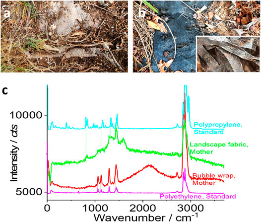
FIGURE 1. Two sampling sites (A, B) and the typical Raman spectra (C). Microplastics might be released from the buried “mother matrix,” including the white bubble wrap (A) and the black landscape fabrics (B). (C) The typical Raman spectrum collected from the “mother matrix.” For comparison, the standard Raman spectra of polyethylene and polypropylene are also presented.

In this study, two types of soil samples around the plastic items were collected, including 1) a white bubble wrap of polyethylene that has been buried under wood mulches for 7 years, due to inappropriate discarding and 2) a black landscape fabric of polypropylene (to control weeds) that has been used as a mulch bed for 7 years. The garden history suggested that the mulch was paved in the summer of 2013.

Sample Preparation On-Site in the Backyard Garden

Soil samples of ∼10 g were mixed with ∼100 ml of tap water. After removing the large items using stainless tweezers, a spoon of table salt (5–10 g) was added to increase the density of water and to help floating of the microplastics. After stirring with a wood stick to reach salt saturation, some salt precipitated at the bottom and was mixed with the soil, which is acceptable.

The floating items were collected with a filter of 0.75 mm first and then with another filter of 100 μm. These filtration processes can be conducted in the backyard garden directly.

The samples collected in the filters were washed with tap water at least 3 times. They were air-dried and transported to a glass slide for the Raman test, and the amount was calculated using microscopy, in duplicates.

Note that this sample preparation approach might not yield a 100% recovery of the microplastics, because 1) some microplastics and nanoplastics were still embedded in the soils and sediments and so they could not float on the water surface for collection and 2) during the sample preparation process, some microplastics were found to be released from large fragments (>5 mm), as shown in Supplementary Figure S3 (Supporting Information).

Sample Preparation Off-Site in the Lab

To increase the signal-to-noise ratio and to collect small microplastics, another sample preparation was carried out in the laboratory. In this case, the tap water was replaced with MQ water and table salt was replaced with zinc chloride. In the meantime, chemical washing was introduced using ethanol.

In brief, soil samples of ∼10 g were mixed with MQ water of ∼50 ml and saturated with zinc chloride. The floating items were collected with a filter of 0.75 mm first, followed by 100 μm and 0.8 μm filters. The collected samples were washed with MQ water three times and then with ethanol three times. They were air-dried and transported to the glass slide for the Raman test. For the sample filtered with a 0.8 μm porous silver membrane, this transport was found unnecessary, as indicated later.

For the Raman test, use of glass slides is a good choice owing to their clean background. Before the distribution of microplastics on its surface, the glass slide had been cleaned by dipping in a piranha solution (2:1 H₂SO₄: H₂O₂, v/v) (warning: this solution reacts vigorously with organic compounds).

Sample Pretreatment in the Lab

To further increase the signal-to-noise ratio, chemical digestion was introduced, particularly for the analysis of microplastics in the size range of 0.8–100 μm. In this case, the liquid obtained after filtering with a 100 μm filter was digested using H₂O₂ at 3% for 24 h at 50°C. Then, a similar protocol was followed, intended to enhance the Raman signal by decreasing the spectrum background by cleaning the surface.

Blank Samples

For the QA/QC control, blank samples were prepared, including the backyard garden and the laboratory. In the backyard garden, a blank sample was prepared in parallel without the soil sample to check the possible contamination from the table salt and tap water. In the laboratory, similarly, the blank sample was prepared using only MQ water. We did collect a tiny amount of microplastics (<10) in the blanks, which is not comparable with the amount of microplastics obtained from the garden, as reported herein. This blank sample was also validated in a commercial laboratory (Eurofins, Australia).

Raman Spectra

The Raman spectra were recorded in the air using a WITec confocal Raman microscope (Alpha 300RS, Germany) equipped with a 532 nm laser diode (<30 mW), as reported before (Sobhani et al., 2019; Sobhani et al., 2020b; Fang et al., 2020). In general, a charge-coupled device detector was used to collect Stokes–Raman signals under a 20×, 40×, or 100× objective lens at room temperature (∼24°C).

To map the image, a piezo-driven scanning stage was employed for each Raman signal collection at each pixel, which was varied by adjusting the moving speed and integration time, from 1 μm × 1 μm to 500 nm × 500 nm, 100 nm × 100 nm, or 40 nm × 40 nm, as indicated in the following. Note that the scanning duration was increased accordingly. For example, to image an area of 10 μm × 10 μm, the scanning duration is increased from 100 s (with a pixel size of 1 μm × 1 μm, to collect 100 spectra as a matrix) to 10,000 s (with a pixel size of 100 nm × 100 nm, to collect 10,000 spectra as a matrix) and to 62,500 s (with a pixel size of 40 nm × 40 nm, to collect 62,500 spectra as a matrix) if each pixel takes 1 s of integration to collect the Raman signal as a Raman spectrum.

For Raman image mapping, the different plastics exhibit different Raman activities and emit different intensities of Raman spectra, as suggested before (Sobhani et al., 2019). For example, the Raman signal at 2,890 cm⁻¹ was collected to image polyethylene, along with other characteristic peaks of fingerprint at 1,060, 1,120, 1,300, and 1,440 cm⁻¹. The intensities at different peaks were mapped as different images.

The collected Raman signal was analyzed using WITec Project software. By just collecting the net intensity of the unique/characteristic peaks for image mapping, the interference which might originate from the spectrum background noise (such as fluorescence), or organic matter, can be effectively avoided by subtracting the baseline of the collected Raman spectra (the peak area or sum, after automatic integration via software) at the selected peaks. The background has been generally subtracted using the collected signal at both sides of the selected Raman peak at the pixels as the spectrum background. To further avoid the “bias and false” imaging, an imaging-algorithm analysis is recommended.

Image Analysis: Logic-Based Algorithm

From the Raman spectra matrix, several images were simultaneously mapped from the same spectrum at different peaks, such as for polyethylene at 1,060, 1,120, 1,300, 1,440, and 2,890 cm⁻¹. At these peak positions, the intensity signal can be mapped as different colors of images. Two or more images as parent images, which correspond to two or more different characteristic peaks, can be merged as a daughter image, either by logic-OR or logic-AND.

For the algorithm analysis, we employed ImageJ software. In general, the parent Raman images are opened by the software and processed and merged with a calculator of logic-OR or logic-AND.

In the case of “logic-OR,” any mapped signal (or dot or pixel) from any image (parent images) will be fetched and merged into a new image (daughter image). Obviously, any “bias and false” noise from the parent images (mapped at two different Raman peaks) might be collected. However, the advantage is that it can significantly reduce signal loss.

In the case of “logic-AND,” the parent Raman images are opened by the software and converted from red-green-blue (RGB) to an 8-bit format. Then, the images are processed and merged with a calculator of logic-AND. After merging, the new image is painted to the selected color in the displaying value range of 0–100, which can be converted back to the RGB format as the daughter image. The image certainty is increased statistically.

Results and Discussion

Sampling and the Mother Matrix

In this study, we tested two soil samples and their sampling sites are shown in Figures 1A,B. The primary material is made of either polyethylene or polypropylene, as suggested by its Raman spectra from the “mother matrix” (brand new from the market) in Figure 1C. During the fabrication process of the “mother matrix,” some pigments or dyes might be formulated to control the color of the products and some additives might be introduced as well to enhance the properties. Consequently, from Figure 1C, it can be seen that it is difficult to get the exactly matched spectrum with the standard ones including polypropylene and polyethylene.

In the meantime, the broad peaks for black carbon, which appear at ∼1,360 and ∼1,580 cm⁻¹ (Dychalska et al., 2015), were observed from the black landscape fabrics. Fortunately, the prominent characteristic peaks for polypropylene (green) and polyethylene (red), along with the broad peak at 2,890 cm⁻¹ (that is assigned to the C-H bond), can be observed for the landscape fabrics and bubble wrap, as marked in Figure 1C. These peaks are marked with dashed lines and selected to identify microplastics as given in the following.

From the spectra shown in Figure 1C, we confirm that the items in Figures 1A,B and their mother matrices are mainly made of plastics, including polypropylene and polyethylene. We then tried to collect their degradation products, the released small fragments or microplastics, formed after 7 years in the garden. Note that these samples might not be representative and vary from gardens to gardens, depending on the ageing, weathering, soil properties, planting, etc. In this case study, however, we intend to collect the released microplastics from the mother matrices to monitor their breakdown fate in one garden.

Bubble Wraps

Microplastics in the Range of 5–0.75 mm, Without Pretreatment

Figure 2 shows the characterization of microplastics released from the bubble wrap in the size range from 0.75 to 5 mm, which is visible to our naked eyes and through a smartphone camera as well. As shown in Figure 2A, from the photo image taken with a smartphone, we can assign the floating items on the water surface to microplastics, which are transparent slight-white fragments. A general estimation is that there are ∼150 pieces of microplastics in a ∼10 g sample. This number is significant, and the potential contamination should be avoided. That is, the bubble wrap should be collected and should not be mixed with the mulch, as the wrongdoing shown here.

FIGURE 2

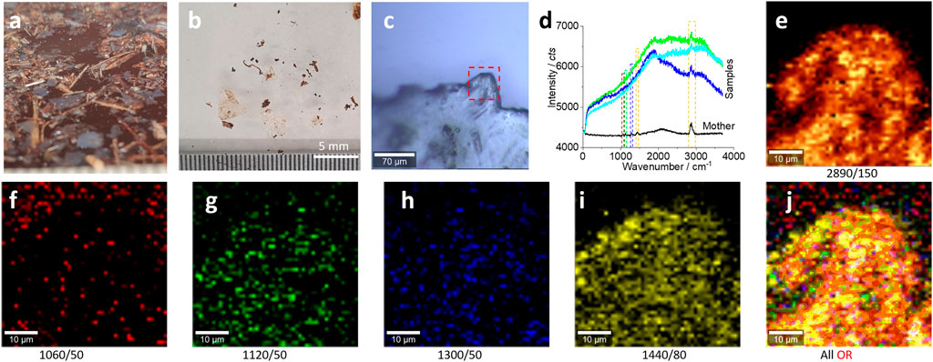
FIGURE 2. Microplastics (without pretreatment) in the range of 5–0.75 mm released from the bubble wrap and their characterizations. (A) The floating microplastics on the water surface, as transparent (slight white) films/fragments. After drying, the sample was distributed on a glass surface for the Raman test (B, C). (D) The typical Raman spectra collected from the squared area in (C) for images (E–J). All Raman spectra were collected with an objective lens of 20×, for a scanning area of 50 μm × 50 μm, with a pixel of 1 μm × 1 μm and integration time of 1 s. The intensity images (E–I) are mapped at the characterized peaks, as marked (and the peak width), with 10% color off-setting. (J) An image after merging all the intensity images (E–I) using logic-OR.

As shown in Figures 2B,C, the photo images were recorded during the Raman test process. The typical spectra are shown in Figure 2D. When compared with the spectra of the “mother matrix,” only the main peak at 2,890 cm⁻¹ can be identified clearly. Consequently, the mapped patterns in Figure 2E are well matched with the photo image squared in Figure 2C, suggesting the existence of the microplastics.

As can be seen from Figure 2D, the other characteristic peaks (squared) of polyethylene from the collected microplastics are weak. However, we can still map their intensities as images. Figures 2F–I show the generated intensity images at the selected peaks for polyethylene. We can see the matched patterns of images with those in Figure 2C, including the characteristic peaks at 1,060 cm⁻¹ (f), 1,120 cm⁻¹ (g), 1,300 cm⁻¹ (h), and 1,440 cm⁻¹ (i) (Sobhani et al., 2019). The reason for this successful image is that these images are generated from the Raman scanning spectrum matrix, which contains 50 × 50 spectra. When the peak intensity is obtained by integration, accumulation, and averaging of the peak area, the signal-to-noise ratio can be enhanced significantly. After mapping as an image, the signal-to-noise ratio of the image is different from that of a single spectrum (50 × 50 vs. 1), from the statistical point of view.

Using logic-OR, we can merge all these images into one (Fang et al., 2021c). The imaged pattern is much clear, as shown in Figure 2J. In effect, all the images in Figure 2E,G–J show the well-matched pattern with those in Figure 2C, except the image in Figure 2F. This is because the peak at 1,060 cm⁻¹ is intrinsically weaker than other peaks, as observed in Figure 1D.

From the results in Figure 2, we can see the success of the capture of microplastics, in the range of 0.75–5 mm, even without special pretreatment. When the size shrinks, the test results are different as reported in the following.

Microplastics in the Range of 0.75 mm–100 μm, Without Pretreatment

Figure 3A shows a photo image of the collected samples in the range of 5–0.75 mm (left) and 0.75 mm–100 µm (right). In this part, we focus our test on the microplastics in the range of 0.75 mm–100 μm. The sample was transported to a glass surface, as shown in Figure 3B. The photo image under the microscope is shown in Figure 3C for the Raman test.

FIGURE 3

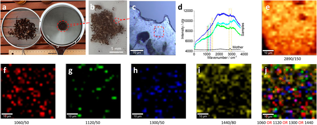
FIGURE 3. Microplastics (without pretreatment) in the size range of 0.75 mm–100 µm released from the bubble wrap and their characterizations. (A) The collected microplastics after drying using a net (left) to collect samples in the range of 5–0.75 mm and a coffee filter (right) to collect samples in the range of 0.75 mm–100 μm, respectively. The latter were distributed on a glass surface for the Raman test (B, C). (D) The typical Raman spectra collected from the squared area in (C) for images (E–J). All Raman spectra were collected with an objective lens of 20×, for an area of 50 μm × 50 μm, with a pixel of 1 μm × 1 μm and integration time of 1 s. The intensity images (E–I) are mapped at the characterized peaks, as marked [and the peak width as well, also squared in (D)], with 10% color off-setting. (J) A merged image of (F–I) using logic-OR.

Under the microscope, it is estimated that there are ∼136 pieces of microplastics in ∼10 g soil in the range of 100 μm–0.75 mm. This estimated amount is comparable with ∼150 pieces of microplastics in 10 g soil in the range of 5–0.75 mm, which can witness the degradation fate of the bubble wrap, from larger ones to smaller ones. In other words, we can collect microplastics (5 mm–100 µm) from our garden using kitchenware, that is, ∼28.6 pieces of microplastics per gram soil.

Similarly, the Raman spectra in Figure 3D can confirm the existence of plastics, particularly in Figure 3E, to map the peak at 2,890 cm⁻¹. The images in Figures 3F–J, which map other characteristic peaks of polyethylene in Figure 3D, further confirm the presence of plastics in the scanning area.

There might be some organic matter on the plastic surface, given the simple sample preparation was conducted on-site in our backyard garden. This might be the reason why there is a strong spectrum background in the Raman spectrum shown in Figure 3D and the reason why the images in Figures 3F–I just show a few bright dots. However, even though the signal of microplastics is weak and might be shielded by the background, as shown in Figures 3E–I, we can assume that the scanning area is mainly made of microplastics. This assumption can be observed clearly in Figure 3J, when the images (f–i) have been merged together to enhance the mapping certainty via enhancing the signal-to-noise ratio.

Therefore, Raman mapping is recommended for microplastic characterization. From the statistical point of view, the intensity image contains the signal from the Raman spectrum matrix, which includes 2,500 spectra here. Consequently, the signal-to-noise ratio for an image is different from that for an individual spectrum, even for a single peak from this individual spectrum. This is why the images in Figures 3E–J can analyze the microplastics, while the spectrum in Figure 3D is difficult to analyze.

Microplastics in the Range of 100–0.8 μm, With Pretreatment

The signal-to-noise ratio is weak in Figures 2D, 3D. When the size of microplastics shrinks, it becomes difficult to identify them. In order to increase the signal-to-noise ratio, we employed the sample pretreatment. To this end, we intend to decrease the noise by cleaning the surface of the microplastics, via digestion using H₂O₂ and washing using organic solvents such as ethanol. The results are presented in Figure 4. This pretreatment should be carried out in a laboratory rather than in the backyard. Without this kind of sample pretreatment, although we can still analyze the microplastics, as shown in Supplementary Figure S4 (Supporting Information), it is difficult to identify them due to the low signal-to-noise ratio.

FIGURE 4

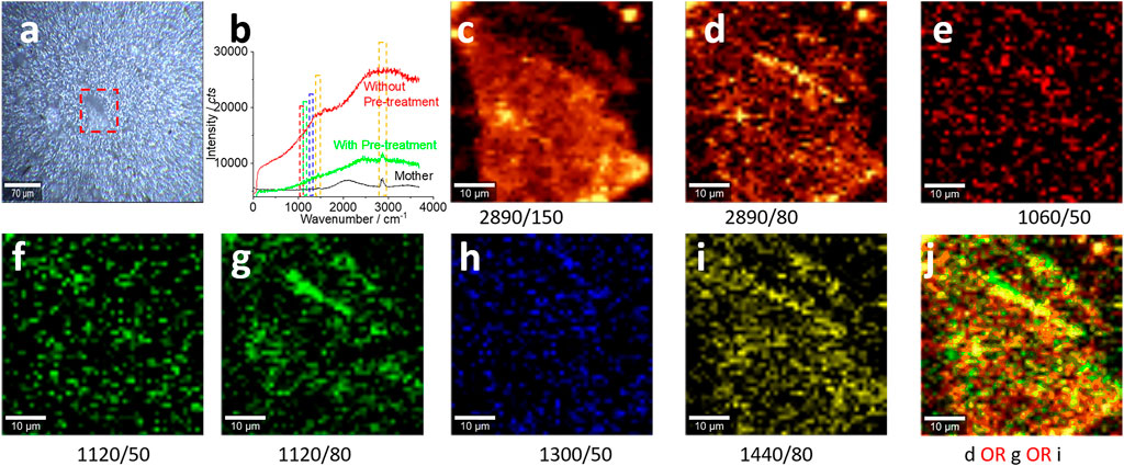
FIGURE 4. Microplastics (with pre-treatment) in the size range of 100–0.8 μm and their characterizations. (A) A photo image of the collected microplastics on the silver membrane surface for the Raman test in (B–J). All Raman spectra were collected with an objective lens of 20×, for an area of 50 μm × 50 μm, with a pixel of 1 μm × 1 μm and integration time of 1 s. The intensity images (C–I) are mapped at the characterized peaks, as marked (and the peak width as well), with 10% color off-setting. (J) A merged image using logic-OR.

Figure 4A shows a photo image by microscopy. The samples were not transported to the glass surface but localized on the silver membrane/filter surface. Figure 4B shows the enhanced spectrum after the sample pretreatment (green curve), particularly for the peak at 2,890 cm⁻¹. Compared to the spectrum collected before the sample pretreatment (black curve), the background fluorescence after the pretreatment is significantly decreased. In the meantime, the peak at 1,560 cm⁻¹ becomes apparent, which is assigned to black carbon (Dychalska et al., 2015). Consequently, the mapped images in Figures 4C–I are presented with a higher certainty, suggesting the success of the sample pretreatment.

When the Raman signal is weak, we should be careful in selecting the peak width to integrate the peak intensity with image generation. The reason is that the weak Raman signal can experience a gentle shift on the peak position. Consequently, by comparing the image in Figure 4C with that in Figure 4D, we can see the slightly changed pattern when the peak width is narrowed from 150 cm⁻¹ to 80 cm⁻¹. Similarly, an improvement from the image in Figure 4F to the image in Figure 4G is achieved by broadening the peak width from 50 to 80 cm⁻¹. Therefore, we require caution in the selection of the peak position and width to avoid signal loss.

Even so, the signal-to-noise ratio is still low. While we need to enhance the ratio further, we might also keep in mind that this issue is difficult to be avoided for the environmental sample. Ageing and weathering make the surface of microplastics covered with organic matter. From Figure 4A, we can even know the scanning area is occupied by the bubble wrap fragment, and the mapped images in Figures 4C–J only generate the blurred profile of the fragment. Due to the low signal-to-noise ratio, logic-OR, rather than logic-AND, is recommended to merge the images, as presented in Figure 4J. Logic-AND might lead to significant signal loss.

For confocal Raman spectroscopy, on the contrary, the Raman signal is mainly collected from the focusing plane, as discussed before (Sobhani et al., 2019). When the plastic fragment is thick and the surface is rough, under the confocal Raman spectroscopy, the top and the bottom parts of the same plastic fragments are not localized on the same focus plane (along the z-axle). If we focus on the top of the microplastic, the bottom part cannot be effectively mapped and thus will be omitted in the mapping image and vice versa; when focus is on the bottom part, the top cannot be mapped effectively. That is, the possible reason for the blurred mapping profile in Figure 4 is that the scanning area is not flat to be localized on the same plane.

We recommend mapping the image for microplastic analysis. The reason has been discussed above and summarized as follows: 1) The signal-to-noise ratio averaged from a matrix of the Raman spectrum is significantly higher than that from an individual Raman spectrum and a single peak. 2) The multipeak mapping can generate multi-images. While the individual image can be used to justify the microplastic, multi-images can be merged for cross-checking, such as by the logic-based algorithm, to increase the analysis certainty. 3) As obtained from the image, if the scanning area is uniformly made of the same material, position identification of one area can be expanded to the whole area, as shown inFigures 3J and 4J. That is, the blurred pattern with bright dots can be considered to represent a whole unique item within the available profile or boundary. Further research is needed here.

In Figure 4A, a window view is of 0.35 mm × 0.3 mm in size, containing ∼15 pieces of microplastics (per 0.105 mm²). The silver membrane is of a diameter of 13 mm (∼133 mm²), which has been employed to collect the microplastics in this range of 0.8–100 μm. Therefore, there are around 1.9 × 10⁴ pieces of microplastics in this range if they are uniformly collected and distributed on the silver filer surface. This number is much higher than that of the large pieces (∼286), suggesting the breakdown pathway from the “mother” item, a large bubble wrap at the very beginning. That is, after the large wrap has been subject to 7 year’s breakdown, which deteriorate the wrap, akin ant-chewing from the peripheral to form a sawtooth boundary, small pieces can be easily released as microplastics, as shown in Supplementary Figure S3 (Supporting Information).

This kind of test needs much research because of the difficulty to find nanoplastics, mainly due to the low signal-to-noise ratio. Therefore, the test for nanoplastics needs more research, particularly for the environmental samples.

Landscape Fabrics

Microplastics in the Range of 5–0.75 mm, Without Pretreatment

Similarly, we tried to collect microplastics released from landscape fabrics. In Figure 1B, we can see the original width of the fabric is ∼2 mm. The spectrum in Figure 1C suggests that the fabric is made of polypropylene mainly, with a background either from the black carbon (Dychalska et al., 2015) or from the fluorescence. After serving as the mulch bed to cover the soil ground for 7 years, fragments were released as microplastics, as shown in Figure 5.

FIGURE 5

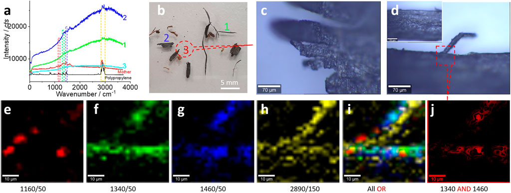
FIGURE 5. Microplastics (without pretreatment) in the range of 5–0.75 mm released from the landscape fabric and their characterizations. (A) The typical Raman spectra and the comparison with the spectra of standard polypropylene and the mother matrix. (B) The positions to collect the Raman spectra in (A). Among them, item #1 is zoomed in (D), #2 is a mulch, and #3 is zoomed in (C). In (D), the square area is scanned for the Raman mapping images (E–H) at the characteristic peaks, as marked (and the peak width), with 10% color off-setting. (I, J) The merged images of the selected Raman images using logic-OR or logic-AND, as indicated. The Raman spectra were collected with an objective lens of 20×, for an area of 50 μm × 50 μm, with a pixel of 2 μm × 2 μm and integration time of 2 s.

Figure 5A shows the typical Raman spectra recorded from the samples, which are positioned in Figure 5B. Figure 5B shows the typical fragments collected by us, where one is longer than 5 mm, considered as macroplastics, and the rest are generally categorized as microplastics, from fibers to irregular fragments, as shown in Figures 5C,D. The fractured parts in Figure 5C suggest the breakdown process of the fabric. This fracture can also be confirmed from the structure shown in Figure 5D, where another fiber (with a diameter or width of ∼12 μm) has been fractured from the fabric trunk. All these microplastics might be released and fractured from the original fabric with a width of ∼2 mm.

To further confirm the released microplastics, we scan the squared area in Figure 5D and map the Raman intensity images again. The selected peaks have the characteristics of polypropylene. In Figures 5E–H, the mapped pattern is well matched with that in Figure 5D, confirming the presence of microplastics of polypropylene. Because the surface of the microplastics had not been effectively cleaned, some organic matter or derived groups might interfere with the Raman test. This is the reason why the mapping images just yield the boundary or the profile. Another reason for the blurred image is that the confocal Raman spectra just collects the signal from the focus plane, which is localized at the boundary, as mentioned above.

Using logic-OR, we can merge all the obtained images and generate an image as shown in Figure 5I, further confirming the presence of microplastics of polypropylene. To increase the image certainty, we generated an image shown in Figure 5J, using logic-AND by merging two images (Figures 5f, g) with strong signals. By doing so, we can cross-check the existence of microplastics. In other words, the image certainty has been increased, from the statistical point of view again.

Microplastics in the Range of 0.75 mm–0.8 μm, Without Pretreatment

When the released polypropylene microplastics shrink in size, the Raman identification gets more complicated. Unlike the bubble wrap that is transparent/white which is easy to be identified and localized under the optical microscope for characterization, the black landscape fabric’s microplastics are mixed with soil, black matter, plant roots, etc. The signal-to-noise ratio is decreased, too. Overall, when the size shrinks, it becomes difficult to characterize the microplastics.

To simplify the analysis process, we fix the Raman mapping parameters, which have been employed in Figure 5, to generate two images individually and merge them together via logic-AND. The different sizes of microplastics are mapped in Figure 6, including the size range of 0.75 mm–100 μm (a, b) and 100–0.8 μm (c, d). The pattern of images in Figures 6B,D are well matched with the pattern in Figures 6A,C , suggesting the success of the capture of the microplastics.

FIGURE 6

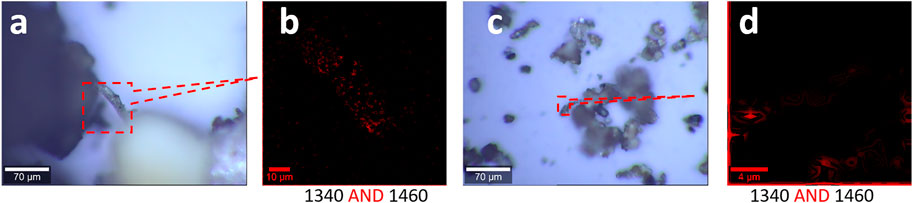
FIGURE 6. Microplastics (without pretreatment) in the range of 0.75 mm–0.8 μm released from the landscape fabric and their characterizations, including photo images (A, C) and Raman images (B, D). (A, B) Results in the size range of 0.75 mm–100 μm. (C, D) Results in the size range of 100–0.8 μm. The Raman spectra were collected with an objective lens of 40×, with a pixel of 1 μm × 1 μm and integration time of 1 s, with 10% color off-setting. Both Raman images are the merged image of the two images mapped at the marked peaks using logic-AND.

In general, we can collect the microplastics, although the image certainty varies. This mapping and merging approach via the logic algorithm is reckoned for microplastic analysis, in particular, when the signal is weak.

Microplastics in the Range of 100–0.8 μm, With Pretreatment

In order to increase the signal-to-noise ratio, again, we performed the pretreatment of the microplastics in the range of 100–0.8 μm, and the results are presented in Figure 7. Figures 7A,B show the effect of the focus plane, where (a) is focused on the top of the large fragments, while (b) is focused on the bottom of them and also the surface of the silver membrane that has been employed as the filter to collect the microplastics. The different focusing planes are the main reason why the confocal Raman spectroscopy cannot map all the fragments, as shown in Figures 7D–G.

FIGURE 7

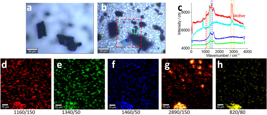
FIGURE 7. Microplastics (with pretreatment) in the range of 100–0.8 μm released from the landscape fabric and their characterizations. (A, B) The effect of the focusing position at the top (A) or at the bottom (B), where (B) is selected to collect the Raman signal by confocal Raman spectroscopy. (C) The typical Raman spectra collected from the marked positions in (B). All Raman spectra were collected with an objective lens of 40×, for an area of 85 μm × 85 μm, with a pixel of 1.75 μm × 1.75 μm and integration time of 1 s. The intensity images (D–G) are mapped at the characterized peaks, as marked (and the peak width), with 10% color off-setting. (H) The background that might be assigned to other items.

Compared with the sample without pretreatment shown in Figures 6C,D, for the analysis in the same size range, the samples in Figure 7 were not transported to the glass surface. Also, after the pretreatment, the microplastics have been concentrated to some degree and the identification of the microplastics becomes easier than that shown in Figure 6. As can be seen from Figure 6C, most of the items are usually soil and organic matter. However, in Figures 7A,B, most items are identified as microplastics. Figure 7C shows the Raman spectra that have been collected on the indicated positions in (b). Basically, the signal-to-noise ratio has been improved, compared with that before the pretreatment.

Even so, the mapping images in Figures 7D–G just show the profile of the fragments. Among these images, Figure 7G yielded a higher (more bright) signal-to-noise ratio, which is due to the strong signal at the peak of C-H. This pattern is matched with that in Figure 7B. Some extra-mapped “fragments” might be the false positives and false negatives produced due to the low signal-to-noise ratio. On the contrary, the resolution of the photo image in Figure 7B is not high enough to visualize all small microplastics and nanoplastics, while the Raman image can, which is the advantage of the Raman mapping (Fang et al., 2020; Fang et al., 2021c). Again, we recommend mapping, rather than of an individual Raman spectrum, to analyze microplastics particularly, when the signal-to-noise ratio is low, such as for the environmental samples, as shown here. As mentioned above, within the scanning area, identification of one position and assignment of the microplastic can be expanded to a whole fragment, such as the bright position mapped on the middle-bottom part of the images. The cross-check in Figures 7D–G can assume that the microplastics are presented at the middle-bottom part, which can be expanded to the whole fragment in Figure 7B to assume that the large fragment is made of plastic as well.

However, the image in Figure 7H might be assigned to other items, such as slat or other interference sources (Sobhani et al., 2019; Sobhani et al., 2020b), which needs more research.

We can also estimate the amount of the released microplastics, and the results are shown in Figure 8. Admittedly, the estimation suffers from significant variations, particularly for the small ones in the range of 100–0.8 μm, and the test for the nanoplastics (<0.8 μm) is not available here. Generally, small fragments (100–0.8 μm) attain a higher number than large ones. The reason has been discussed earlier and shown in Supplementary Figure S3 (Supporting Information). Furthermore, unlike the wrongly discarded bubble wrap that is just a small piece at the beginning as the “mother,” the landscape fabric can cover the whole garden. In this case, for a covered area of 1 m² in our garden, the released amount of microplastics can reach hundreds of millions, according to our estimation.

FIGURE 8

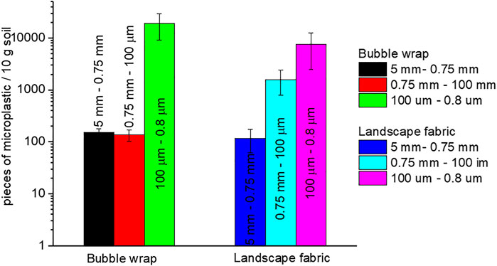
FIGURE 8. Amount of the released microplastics.

Conclusion

We demonstrate here that we can collect microplastics from our gardens, via a simplified sample preparation process of Raman imaging, as a case study. We consider the Raman imaging and logic-based algorithm to increase the signal-to-noise ratio and the image certainty. This approach is helpful in analyzing the weak signal of the environmental samples, particularly when the signal is almost shielded by the background.

We also show that the release of microplastics in our garden is profound, either due to the wrongly discarded plastic items such as bubble wrap or due to the use of plastic items such as landscape fabrics as the mulch bed. Although the nanoplastic characterization is not available in this study, the released amount is expected to be significant. For example, a piece of plastic at a size of 5 mm × 5 mm × 5 mm is equivalent, in mass or weight, to 1 × 10⁹ pieces of microplastics at a size of 5 μm × 5 μm × 5 μm or equivalent to 1 × 10¹⁸ pieces of nanoplastics at a size of 5 nm × 5 nm × 5 nm. Therefore, if we care about the contamination from microplastics and nanoplastics, we must be very cautious about the use of plastic items in our garden.

Data Availability Statement

The original contributions presented in the study are included in the article/Supplementary Material; further inquiries can be directed to the corresponding author.

Author Contributions

CF, MM, and RN were involved in experiment design and management. ZS and CG participated in data collection and sample preparation. YT and YL supported the manuscript preparation and reviewing process.

Funding

The authors appreciate the funding support from the CRC CARE and the University of Newcastle, Australia.

Conflict of Interest

The authors YL, RN, MM, and CF are employed at CRC CARE Pty Ltd.

The remaining authors declare that the research was conducted in the absence of any commercial or financial relationships that could be construed as a potential conflict of interest.

Publisher’s Note

All claims expressed in this article are solely those of the authors and do not necessarily represent those of their affiliated organizations, or those of the publisher, the editors, and the reviewers. Any product that may be evaluated in this article, or claim that may be made by its manufacturer, is not guaranteed or endorsed by the publisher.

Acknowledgments

For the Raman measurements, the authors acknowledge the use and support of the South Australian node of Microscopy Australia (formerly known as AMMRF) at Flinders University, South Australia.

Supplementary Material

The Supplementary Material for this article can be found online at https://www.frontiersin.org/articles/10.3389/fenvs.2021.739775/full#supplementary-material

References

Andrady, A. L. (2017). The Plastic in Microplastics: A Review. Mar. Pollut. Bull. 119 (1), 12–22. doi:10.1016/j.marpolbul.2017.01.082

PubMed Abstract | CrossRef Full Text | Google Scholar

Arthur, C., Baker, J. E., and Bamford, H. A. (2009). in Proceedings of the International Research Workshop on the Occurrence, Effects, and Fate of Microplastic Marine Debris, September 9-11, 2008 (Tacoma, WA, USA: University of Washington Tacoma).

Browne, M. A. (2015). “Sources and Pathways of Microplastics to Habitats,” in Marine Anthropogenic Litter (Springer), 229–244. doi:10.1007/978-3-319-16510-3_9

CrossRef Full Text | Google Scholar

Cox, K. D., Covernton, G. A., Davies, H. L., Dower, J. F., Juanes, F., and Dudas, S. E. (2019). Human Consumption of Microplastics. Environ. Sci. Technol. 53 (12), 7068–7074. doi:10.1021/acs.est.9b01517

PubMed Abstract | CrossRef Full Text | Google Scholar

Dychalska, A., Popielarski, P., Franków, W., Fabisiak, K., Paprocki, K., and Szybowicz, M. (2015). Study of CVD diamond Layers with Amorphous Carbon Admixture by Raman Scattering Spectroscopy. Mater. Science-Poland. 33, 799–805. doi:10.1515/msp-2015-0067

CrossRef Full Text | Google Scholar

Fang, C., Luo, Y., Zhang, X., Zhang, H., Nolan, A., and Naidu, R. (2021a). Identification and Visualisation of Microplastics via PCA to Decode Raman Spectrum Matrix towards Imaging. Chemosphere 286, 131736. doi:10.1016/j.chemosphere.2021.131736

PubMed Abstract | CrossRef Full Text | Google Scholar

Fang, C., Sobhani, Z., Zhang, D., Zhang, X., Gibson, C. T., Tang, Y., et al. (2021b). Capture and Characterisation of Microplastics Printed on Paper via Laser Printer's Toners. Chemosphere 281, 130864. doi:10.1016/j.chemosphere.2021.130864

PubMed Abstract | CrossRef Full Text | Google Scholar

Fang, C., Sobhani, Z., Zhang, X., Gibson, C. T., Tang, Y., and Naidu, R. (2020). Identification and Visualisation of Microplastics/Nanoplastics by Raman Imaging (Ii): Smaller Than the Diffraction Limit of Laser? Water Res. 183, 116046. doi:10.1016/j.watres.2020.116046

PubMed Abstract | CrossRef Full Text | Google Scholar

Fang, C., Sobhani, Z., Zhang, X., McCourt, L., Routley, B., Gibson, C. T., et al. (2021c). Identification and Visualisation of Microplastics/Nanoplastics by Raman Imaging (Iii): Algorithm to Cross-Check Multi-Images. Water Res. 194, 116913. doi:10.1016/j.watres.2021.116913

PubMed Abstract | CrossRef Full Text | Google Scholar

Gigault, J., Halle, A. t., Baudrimont, M., Pascal, P.-Y., Gauffre, F., Phi, T.-L., et al. (2018). Current Opinion: What Is a Nanoplastic? Environ. Pollut. 235, 1030–1034. doi:10.1016/j.envpol.2018.01.024

PubMed Abstract | CrossRef Full Text | Google Scholar

Hartmann, N. B., Skjolding, L. M., Nolte, T., and Baun, A. (2016). Aquatic Ecotoxicity Testing of Nanoplastics-Lessons Learned from Nanoecotoxicology. SETAC Europe, 43–44.

Ivleva, N. P., Wiesheu, A. C., and Niessner, R. (2017). Microplastic in Aquatic Ecosystems. Angew. Chem. Int. Ed. 56 (7), 1720–1739. doi:10.1002/anie.201606957

PubMed Abstract | CrossRef Full Text | Google Scholar

Koelmans, A. A., Mohamed Nor, N. H., Hermsen, E., Kooi, M., Mintenig, S. M., and De France, J. (2019). Microplastics in Freshwaters and Drinking Water: Critical Review and Assessment of Data Quality. Water Res. 155, 410–422. doi:10.1016/j.watres.2019.02.054

PubMed Abstract | CrossRef Full Text | Google Scholar

Liebezeit, G., and Liebezeit, E. (2014). Synthetic Particles as Contaminants in German Beers. Food Additives & Contaminants: A 31 (9), 1574–1578. doi:10.1080/19440049.2014.945099

CrossRef Full Text | Google Scholar

Mattsson, K., Johnson, E. V., Malmendal, A., Linse, S., Hansson, L.-A., and Cedervall, T. (2017). Brain Damage and Behavioural Disorders in Fish Induced by Plastic Nanoparticles Delivered through the Food Chain. Sci. Rep. 7 (1), 11452. doi:10.1038/s41598-017-10813-0

PubMed Abstract | CrossRef Full Text | Google Scholar

Sobhani, Z., Al Amin, M., Naidu, R., Megharaj, M., and Fang, C. (2019). Identification and Visualisation of Microplastics by Raman Mapping. Analytica Chim. Acta 1077, 191–199. doi:10.1016/j.aca.2019.05.021

PubMed Abstract | CrossRef Full Text | Google Scholar

Sobhani, Z., Lei, Y., Tang, Y., Wu, L., Zhang, X., Naidu, R., et al. (2020a). Microplastics Generated when Opening Plastic Packaging. Sci. Rep. 10 (1), 4841. doi:10.1038/s41598-020-61146-4

PubMed Abstract | CrossRef Full Text | Google Scholar

Sobhani, Z., Zhang, X., Gibson, C., Naidu, R., Megharaj, M., and Fang, C. (2020b). Identification and Visualisation of Microplastics/nanoplastics by Raman Imaging (I): Down to 100 Nm. Water Res. 174, 115658. doi:10.1016/j.watres.2020.115658

PubMed Abstract | CrossRef Full Text | Google Scholar

Steinmetz, Z., Wollmann, C., Schaefer, M., Buchmann, C., David, J., Tröger, J., et al. (2016). Plastic Mulching in Agriculture. Trading Short-Term Agronomic Benefits for Long-Term Soil Degradation? Sci. Total Environ. 550, 690–705. doi:10.1016/j.scitotenv.2016.01.153

PubMed Abstract | CrossRef Full Text | Google Scholar

Vroom, R. J. E., Koelmans, A. A., Besseling, E., and Halsband, C. (2017). Aging of Microplastics Promotes Their Ingestion by marine Zooplankton. Environ. Pollut. 231, 987–996. doi:10.1016/j.envpol.2017.08.088

PubMed Abstract | CrossRef Full Text | Google Scholar

Wright, S. L., and Kelly, F. J. (2017). Plastic and Human Health: a Micro Issue? Environ. Sci. Technol. 51 (12), 6634–6647. doi:10.1021/acs.est.7b00423

PubMed Abstract | CrossRef Full Text | Google Scholar

Zhang, L., Sintim, H. Y., Bary, A. I., Hayes, D. G., Wadsworth, L. C., Anunciado, M. B., et al. (2018). Interaction of Lumbricus Terrestris with Macroscopic Polyethylene and Biodegradable Plastic Mulch. Sci. Total Environ. 635, 1600–1608. doi:10.1016/j.scitotenv.2018.04.054

PubMed Abstract | CrossRef Full Text | Google Scholar