An Ensemble Prediction System Based on Artificial Neural Networks and Deep Learning Methods for Deterministic and Probabilistic Carbon Price Forecasting

Introduction

This section describes the research background, provides a literature review, and states the purpose and innovation of this study.

Research Background

With the rapid development of the economy, the environment and the climate will inevitably change. Climate change is clearly a common problem facing all countries. On February 16, 2005, the Kyoto Protocol went into effect. According to the situation in each country, specific emission reduction plans and schedules were formulated. In January 2005, the EU emissions trading scheme (EU ETS), which was designed to achieve the emission reduction targets stipulated in the Kyoto protocol, was introduced (Arouri et al., 2012). The EU ETS allocates carbon trading quotas to different emission entities according to its regulations, and entities that exceed the quota must purchase emission rights from entities that are lower than the quota through the carbon trading market. This measure of using a market trading mechanism provides valuable experience for solving the problem of global climate change.

As the world’s largest carbon dioxide emitter (in 2018, its total carbon dioxide emissions reached 10 billion tons, accounting for approximately 30% of global carbon dioxide emissions), China has successively established eight carbon emission trading markets since 2013. However, this system is still in the construction stage, and the market mechanism is not perfect and needs further improvement. By studying the regular price fluctuation pattern of the EU ETS and China’s carbon trading market, analyzing the influencing factors, and forecasting the carbon market price accordingly, we can better understand the fluctuation law of the carbon market and obtain a reference for formulating carbon market policies and mechanisms to improve the ability to regulate this market.

Carbon prices have important implications for governments, companies, and long-term investors. For governments, carbon pricing is one of the mechanisms used to reduce carbon emissions, and it can also be a source of revenue. Companies can use internal carbon pricing to assess the impact of mandatory carbon pricing on their businesses and to identify potential climate risks and revenue opportunities. Long-term investors are using carbon pricing to reevaluate their investment strategies. Therefore, regardless of the point of view, it is necessary to establish an accurate and stable carbon price forecasting system.

Literature Review

Most of the research methods used in carbon price prediction rely on historical data to build models to predict carbon prices. Carbon prices display high volatility and nonlinear structure, and many studies of carbon price prediction based on historical data have been conducted in recent years. The prediction methods can be divided into three categories: 1) statistical measurement methods; 2) artificial intelligence methods; and 3) decomposition integration hybrid forecasting methods.

Statistical Measurement Method

As a classical time series forecasting method, statistical measurement methods, including linear regression models, autoregressive integrated moving averages (ARIMAs), generalized autoregressive conditional heteroscedasticity (GARCH) models, and gray model GM (1, 1) (Chevallier, 2009; Byun and Cho, 2013; Zhu and Wei, 2013) are widely used in carbon trading price prediction and volatility analysis. For example, Benz and Trück (2008) proposed the Markov transition and AR-GARCH model for stochastic modeling and analyzed the short-term price of the carbon dioxide emission quota of the EU ETS. Through the empirical results obtained, it was demonstrated that the prediction performance of the Markov state transition model is better than that of the GARCH model. Zhu and Wei (2013) combined least squares SVM with the ARIMA model, and the results showed that the developed model was more robust than the single-prediction model. Zhu B et al. (2018) used grey correlation analysis to analyze the carbon price market. The traditional statistical model has high prediction accuracy and wide adaptability in linear and stable time series. However, because carbon prices show strong volatility, nonlinearity, and instability, traditional statistical measurement methods cannot capture internal structural characteristic data (Lu et al., 2019). Therefore, accurate forecasting of carbon prices requires the use of a method with a strong nonlinear feature extraction ability that enables it to take into account potential nonlinear characteristics. In addition, the traditional statistical measurement method is more suitable for the long-term prediction of time series, and its short-term carbon price prediction performance is poor (Cheng and Wang, 2020).

Owing to the shortcomings of statistical models, artificial intelligence methods (AI) have gradually become widely used in time series prediction; these methods are suitable for nonlinear prediction without any assumption of data distribution (Wang et al., 2020). Increasing evidence shows that the performance of AI in nonlinear time series is better than that of other models (Zhang et al., 2017). AI, including back-propagation neural networks (BPs), multilayer perceptual neural networks (MLPs), least squares support vector regression (LSSVR), and hybrid prediction methods combined with optimization algorithms, have also been widely used in carbon price forecasting. Atsalakis (2016) combined a hybrid fuzzy controller called PATSOS with an adaptive neuro fuzzy inference system (ANFIS). The research shows that this method can produce accurate and timely prediction results. Fan et al. (2015) studied the chaotic characteristics of the EU ETS, used the neural network model of MLP to predict carbon prices, and found that the forecasting accuracy of the model was significantly improved. Tian and Hao (2020) used phase space reconstruction technology and the ELM under the multiobjective grasshopper optimization algorithm (MOGOA-ELM) to predict the trend of the EU ETS and China’s carbon prices. The empirical results show that this method can be used effectively to predict carbon prices.

In recent years, with the development of deep learning theory (DL) in image detection, audio detection, and other fields, DL has become the focus of many scholars (Liu et al., 2021). The unique storage unit structure of deep learning allows it to retain past historical data and has significant advantages for processing time series data that feature long processing intervals and delays (Zhang B et al., 2018). Niu et al. (2020) combined LSTM and GRU to establish a deep learning recursive forecasting unit for forecasting multiple financial data. Liu et al. (2020) proposed a new wind speed prediction model based on an error correction strategy and the LSTM algorithm to predict short-term wind speed. The experimental results demonstrated that its performance is better than that of other comparable models. However, application of deep learning frameworks to carbon price prediction is still very limited.

In addition to the selection and optimization of prediction methods, data preprocessing technology also plays an indispensable role in the prediction accuracy of the prediction model (Wang et al., 2021). Decomposition and integration methods, including empirical mode decomposition (EMD), singular spectrum denoising (SSA), and variational mode decomposition (VMD) are widely used in time series data preprocessing. These methods aim to decompose and reconstruct the original time series data and extract the effective features of the time series. Decomposing the original time series into a series of simple patterns that exhibit strong regularity can significantly improve the prediction accuracy of time series. Wei et al. (2018) used wavelet transform and kernel ELM to predict carbon prices. Zhu J et al. (2018) explored an efficient prediction model based on VMD mode reconstruction and optimal combination and thereby greatly improved the prediction accuracy of carbon prices. However, the above decomposition methods still have some shortcomings. For example, in wavelet decomposition and VMD, it is necessary to determine the wavelet basis function and the decomposition level. Although in EMD it is not necessary to determine the number of decomposition levels, mode aliasing and insufficient noise separation cannot be solved (Jin et al., 2020). Therefore, it is very important to extract the nonlinear peculiarities of carbon prices by using appropriate data preprocessing methods.

A single prediction model cannot achieve good performance on every dataset. Therefore, researchers began to focus on combination forecasting models. In essence, combination forecasting models combine different hybrid forecasting methods or single forecasting methods using weighting. In many experimental studies, it is found that the use of a combination of prediction methods produces better predictions than the use of a method that is based on a single-prediction model. The advantage of using combination models is that different time series may have different information sets, information features, and modeling structures, and the use of a combination of prediction methods can result in good performance in the case of such structure mutations. Although the use of a combination forecasting method to forecast time series is very common, use of a combination forecasting model to forecast carbon prices is still in its infancy.

The above analysis indicates that most research on carbon prices is driven by single or hybrid forecasting models and that it tends to emphasize prediction strategies that are based on certainty and to largely ignore the importance of uncertainty analysis of carbon prices. Regardless of the type of prediction model used, there are inherent and irreducible uncertainties in each prediction that will greatly increase the possibility of miscalculation (Du et al., 2020). Therefore, quantification of the uncertainty of carbon price prediction plays an indispensable role in exploring the complexity of the carbon price market and strengthening the ability to conduct effective market anti-risk management.

Objectives and Contributions

To supplement the existing research on carbon price prediction, an ensemble prediction system (EPS) based on the ICEEMDAN data preprocessing method, the deep learning algorithm (DL), the extreme learning machine (ELM), and the multiobjective dragonfly optimization algorithm (MODA) is developed and used to analyze the certainty and uncertainty of carbon prices. Specifically, ICEEMDAN is employed to decompose and reconstruct the original carbon price data and extract the effective features of the data, and the results are transferred into the submodels of EPS as training data (the submodels are ICEEMDAN-GBiLSTM, ICEEMDAN-CNN, and ICEEMDSAN-ELM). Using the MODA, the final carbon price point forecast results are then obtained through a weighted combination of the submodel prediction results. For interval prediction, the upper and lower bounds of the prediction interval are constructed based on the prediction value of ESP and the best fit distribution function of error, namely, the T location-scale (TLS) distribution. The main innovations presented in this study are as follows:

1) An effective ensemble prediction system of carbon prices is developed. Two hybrid prediction models based on a deep learning algorithm (ICEEMDAN-GBiLSTM and ICEEMDAN-CNN) and a feedforward neural network (ICEEMDAN-ELM) are combined to overcome the inherent defects of a single hybrid prediction model.

2) A deep learning recurrent neural network, GBiLSTM, is first proposed as a prediction submodel of the EPS. GBiLSTM combines two recursive deep learning algorithms; it can effectively deal with time series with long memory and increase the accuracy of carbon price forecasting.

3) The MODA is employed as an effective method of weighting the ensemble prediction system. It optimizes the weight coefficient of the ensemble model from the perspective of prediction accuracy and prediction stability, thereby overcoming the obvious defect that single objective optimization can only select one objective function.

4) To overcome the nonlinearity and strong volatility of the original carbon price data, an effective time series preprocessing technique is developed. ICEEMDAN sequence decomposition technology is employed to decompose and reconstruct the original carbon price data, extract the salient features of the data, and improve the prediction accuracy of the EPS.

5) By fitting the best error distribution, the uncertainty of the carbon price is mined. In the past, the error distribution of a prediction was usually assumed to be a Gaussian distribution. In this study, five types of parameter distribution functions are used to fit the prediction error, the best error distribution function is found, and the ranges of carbon price interval prediction are constructed.

The remainder of the study is organized as follows. In Section Model Theory and Related Work and Section Ensemble Prediction System and its Interval Forecasting Framework, we introduce the theoretical method and the framework used in the proposed EPS. Section Experiment and Analysis describes the experimental data and the prediction performance evaluation index. The point prediction and interval prediction of the carbon price are then simulated. Section Discussion is a further discussion of EPS, and a summary of the study is presented in Section Conclusion.

Model Theory and Related Work

This section introduces the corresponding theories and describes the functions of the data preprocessing module, the combination prediction module, and the uncertainty mining module of the EPS prediction system.

Data Preprocessing

The data processing module includes the data feature extraction method, which is based on improved complex ensemble empirical mode decomposition with adaptive noise (ICEEMDAN), and the data feature selection method, which is based on the partial autocorrelation function (PACF).

Data Feature Extraction

To improve the problem of mode aliasing in the traditional noise reduction method EMD and the slight residual noise in CEEMDAN, the ICEEMDAN technology is improved. The CEEMDAN method adds Gaussian white noise during the decomposition process, while the ICEEMDAN method adds a special type of white noise, $E_k({\omega }^{\left(i\right)})$, that is, the k-th IMF component of the Gaussian white noise (M.E. Torres et al., 2011; M.A. Colominas et al., 2014). The local mean value of the added noise is calculated for each modal component, and the IMF is defined as the difference between the residual signal and the local mean.

1) The definition operator $E_k(·)$ represents the k-th IMF after EMD decomposition, and $M(·)$ represents the local mean value of the signal. There is ${\mathit{E}}_1\left(x\right)=x-\mathit{M}\left(x\right)$. Operator means taking the mean value, and x represents the original data of the study, and then the local average value is calculated by EMD:

${\mathit{x}}^{\left(i\right)}=\mathit{x}+{\alpha }_0{\mathit{E}}_1\left({\omega }^{\left(i\right)}\right)(1)$

where ${\omega }^{\left(i\right)}$ is the ith white noise added and ${\alpha }_0$ is the standard deviation of the noise. The first residual component ${\text{r}}_1=\langle M\left(x^i\right)\rangle$ is obtained by taking the local mean value. The first intrinsic mode function IMF₁ value ${\tilde{\mathit{d}}}_1=\text{x}-r_1$ is calculated.

2) The value ${\tilde{d}}_2$ of the second mode component IMF₂ is calculated:

${\tilde{\mathit{d}}}_2=r_1-r_2=r_1-\langle \mathit{M}(r_1+{\alpha }_1{\mathit{E}}_2({\omega }^{\left(i\right)}))\rangle (2)$

3) The k-th residual is calculated:

${\mathit{r}}_{\mathit{k}}=\langle \mathit{M}\left(r_{k-1}+{\alpha }_{k-1}{\mathit{E}}_{\mathit{k}}\left({\omega }^{\left(i\right)}\right)\right)\rangle ,k=\mathrm{2,3},\cdots ,N(3)$

4) The value of the k-th mode component IMF_k:${\tilde{\mathit{d}}}_{\mathbf{k}}=r_{k-1}-r_k$, is calculated, and Eq. 3 is repeated until the residual satisfies the iteration termination condition, which is Cauchy convergence. The standard deviation between two adjacent IMF components $\chi ={\Vert {\tilde{\text{d}}}_k-{\tilde{\text{d}}}_{k-1}\Vert }_2/{\Vert {\tilde{\text{d}}}_{k-1}\Vert }_2$ is less than a specified value.

In this study, ICEEMDAN is used to decompose the original carbon price data into several intrinsic mode functions (IMFs). The IMF with the highest frequency is removed, and the remaining IMFs are included. Through this method of deconstruction and reorganization, the problem of strong volatility and randomness of the original data is solved. The data features are effectively extracted, and the prediction veracity of the model is increased.

Data Feature Selection

The partial autocorrelation function (PACF) is an effective method for distinguishing the structural features of sequences (Jiang et al., 2020). It can be used to calculate the partial correlation between the time series and its lag term. If ${\Phi }_{kj}$ is employed to represent the j-th regression coefficient in the k-order autoregressive equation, the model can be expressed as follows:

${\mathit{x}}_{\text{t}}={\mathit{\Phi }}_{k1}{x}_{t-1}+{\mathit{\Phi }}_{k2}{x}_{t-2}+\cdot \cdot \cdot +{\mathit{\Phi }}_{kk}{x}_{t-k}+{\mu }_t(4)$

where x_t is the time series and ${\Phi }_{kk}$ is the last coefficient. If ${\Phi }_{kk}$ is defined as a function of lag time k, then ${\Phi }_{kk}$, k = 1,2... is named partial autocorrelation function.

In this study, PACF is used to find the lag terms that have the strongest correlation with the time series; these are then used as the input characteristics of the forecast model.

Ensemble Prediction Module

The prediction value calculated by the ensemble prediction system is obtained using an ensemble of the prediction results of different single-prediction components through the weighting strategy. In this section, the three submodes of the proposed EPS and the MODA weighting optimization strategy are introduced.

Convolutional Neural Network

A CNN is an incompletely connected DL network structure that is composed of two special neural networks: a convolution layer and a down sampling layer (Wang, 2020). The neurons in each layer of the CNN are locally connected, enabling them to realize hierarchical feature extraction and transformation of the input. Neurons with the same connection weight are connected to different regions of the upper neural network; in this way, a translation-invariant neural network is obtained (Wang, 2018).

1) The training of the Convolution Layer. The CNN is connected to the local region of the feature surface by a convolution kernel. The output characteristic surface size of each convolution layer must meet the following requirement:

$o\mathit{MapN}=\left(\frac{(i\mathit{Map}n-C\mathit{Window})}{C\mathit{Interval}}+1\right)(5)$

In Eq. 5, oMapN is the number of output feature surfaces of each convolution layer, iMapN is the number of input feature surfaces, CWindow is the size of the convolution kernel, and CInterval is the sliding step size of the convolution kernel.

In general, to ensure integral division in the above formula, it is necessary to train the number of parameters for each convolution layer of the CNN so as to satisfy the following condition:

$\text{C}\mathit{Params}=(i\mathit{Map}\times C\mathit{Window}+1)\times o\mathit{Map}(6)$

where CParams is the number of parameters, iMap is the input feature surface, and oMap is the output feature surface.

The output value $x_{nk}^{out}$can be obtained by the convolution layer; the formula is as follows:

${\mathit{x}}_{\mathit{nk}}^{\mathit{out}}={\mathit{f}}_{\mathit{cov}}\left({\mathit{x}}_{1\mathit{h}}^{\mathit{in}}\times {\mathit{w}}_{1\left(h\right)n\left(k\right)}+{\mathit{x}}_{1(\mathit{h}+1)}^{\mathit{in}}\times {\mathit{w}}_{1(h+1)n\left(k\right)}+{\mathit{x}}_{1(\text{h}+2)}^{\mathit{in}}\times {\mathit{w}}_{1(h+2)n\left(k\right)}+\cdots +{\mathit{b}}_{\mathit{n}}\right)(7)$

where $x_{mk}^{in}$ is the input value, $b_n$ is the offset value of the output characteristic surface n, and$f_{\mathrm{cov}}(\cdot )$ is the excitation function. The excitation function is usually the ReLU function, and the formula for its calculation is as follows:

${\mathit{f}}_{\mathit{cov}}\left(x\right)=\mathit{MAX}\left(0,x\right)(8)$

2) The output of the Pooling Layer. The pooling layer is also composed of several feature surfaces, and the number of feature surfaces does not change. The output value of the pooling layer is

${\mathit{t}}_{\mathit{nl}}^{\mathit{out}}{=\mathit{f}}_{\mathit{sub}}\left(t_{nq}^{in},t_{n(q+1)}^{in}\right)(9)$

where $t_{nq}^{in}$ is the output value of the q-th neuron on the n-th input characteristic surface of the pooling layer and $f_{sub}(\cdot )$ is a function that takes either the maximum value or the mean value. The size DoMapN of each output feature surface of the pooling layer is

$\mathit{DoPapN}=\left(\frac{o\mathit{Map}N}{D\mathit{Window}}\right)(10)$

3) Full connection layer output. In the CNN structure, one or more fully connected layers are connected after the multiple convolution layers and the pooling layers are obtained. The ReLU function is also used in the excitation function of the whole connected layer.

In this study, CNN, as a component of the combined forecasting system, forecasts the carbon price.

Deep Learning Recursive Network Structure (GBiLSTM)

In this study, we developed a deep learning recurrent network structure, which is a hybrid of BiLSTM and GRU. The structure diagram is shown in Figure 1.

FIGURE 1

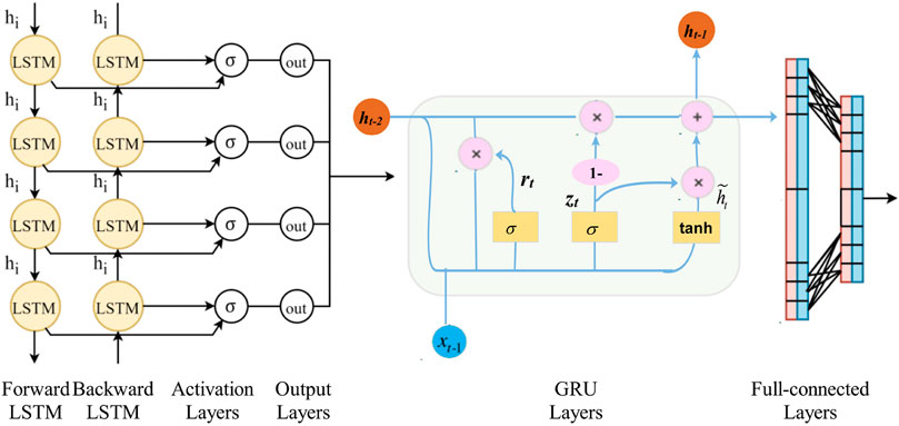
FIGURE 1. Flowchart of the proposed bidirectional long short-term memory-gated recurrent unit (GBiLSTM) model.

Bidirectional Long Short Term Memory Neural Network

BiLSTM is an improved network of LSTM. LSTM cannot capture information from back to front; however, BiLSTM can solve this problem. When bidirectional sequence information is captured, the time series can be predicted more accurately (Hochreiter and Schmidhuber, 1997).

1) The LSTM mechanism consists of three memory gates: an input gate (i_t), a forgetting gate (f_t), and an output gate (O_t). The specific expression is as follows:

$\{\begin{array}{c}{\mathit{i}}_{\mathit{t}}=\sigma ({\omega }_{\mathit{i}}{\mathit{X}}_{\mathit{t}}+R_i{\mathit{H}}_{\mathit{t}-1}+{\mathit{B}}_{\mathit{i}})\\ {\mathit{f}}_t=\sigma ({\omega }_f{\mathit{X}}_{\mathit{t}}+R_f{\mathit{H}}_{\mathit{t}-1}+{\mathit{B}}_{\mathit{f}})\\ {\mathit{o}}_{\mathit{t}}=\sigma ({\omega }_o{\mathit{X}}_{\mathit{t}}+R_o{\mathit{H}}_{\mathit{t}-1}+{\mathit{B}}_{\text{o}})\\ \tilde{\mathit{c}}={\mathit{f}}_t\otimes c_{t-1}\\ {\mathit{H}}_{\mathit{t}}=o_t\otimes \mathit{tanh}\left(c_t\right)\end{array}(11)$

where x_t, $\sigma$, and $c_t$ represent the input sample, the sigmoid activation function, and the storage unit of time t, respectively, and (B_f, B_i, B_o) and (${\omega }_f$, ${\omega }_i$, ${\omega }_o$) represent the deviation and the weight matrix, respectively, of each gate. The symbol $\otimes$ represents the corresponding multiplication of elements. First, ${\mathit{H}}_{\text{t}-1}$, $c_{t-1}$, and ${\mathit{X}}_{\text{t}}$ transmit input information to the LSTM unit. The LSTM gate then interacts with${\mathit{X}}_{\text{t}}$. After a new cell state $c_{t-1}$ is established. In this stage, ${\mathit{f}}_t$ determines which information needs to be stored or deleted and then updates the cell status.

2) Because BiLSTM transmits time series data to LSTM from both the forward and backward directions, it has two output layers: a forward layer $H_t^f=o_t^f\otimes \mathit{tanh}\left(c_t^f\right)$ and a backward layer $H_t^b=o_t^b\otimes \mathit{tanh}\left(c_t^b\right)$.

3) The final predicted output value ${\widehat{y}}_t$ is obtained by integrating the forward layer and the backward layer; in Eq. 12, $\alpha$and $\beta$are numerical factors that satisfy the equation $\alpha +\beta =1$ (Shi et al., 2015).

$\{\begin{array}{c}{\mathit{H}}_{\text{t}}=\alpha {\mathit{H}}_{\text{t}}^{\text{f}}+\beta {\mathit{H}}_{\text{t}}^{\text{b}}\\ {\widehat{y}}_t=\sigma \left({\mathit{H}}_t\right)\end{array}(12)$

Gated Recurrent Unit

GRU is an effective variant of LSTM; its structure is simpler than that of LSTM, and it can well capture the nonlinear relationship between sequence data, thereby effectively alleviating the problems of traditional RNN gradient disappearance (Chung et al., 2014).

1) The GRU model has two gating units: an update gate ${\text{z}}_{\text{t}}$ and a reset gate ${\text{r}}_{\text{t}}$. An update gate is employed to equilibrate the historical information. The smaller the value of the update gate is, the more concentrated the output of the model on the information of the previous hidden layer ${\mathit{h}}_{\text{t}}$ is

${\mathit{Z}}_t=\sigma \left({\mathit{W}}_z.\left[{\mathit{h}}_{\mathit{t}-1\text{,}}{\mathit{x}}_{\mathit{t}}\right]\right)(13)$

${\mathit{r}}_t=\sigma \left({\mathit{W}}_r.[{\mathit{h}}_{\mathit{t}-1},{\mathit{x}}_{\mathit{t}}]\right)(14)$

In Eqs 13, 14, $\text{W}$is the model weight, and $\sigma$ is the activation function.

2) By resetting the gate $r_t$, the candidate vector ${\tilde{\mathit{h}}}_t=\mathit{tanh}(\mathit{W}.[{\mathit{r}}_t\ast {\mathit{h}}_{t-1},{\mathit{x}}_t])$ can be calculated. Taking the value of the update gate as the weight, ${\tilde{\mathit{h}}}_t$ to be added and the state of the hidden layer at the previous time step are recorded as the output of the GRU network at time step t, as follows:

${\mathit{h}}_t=(1-{\mathit{Z}}_t)\ast {\mathit{h}}_{t-1}+{\mathit{Z}}_t\ast {\tilde{\mathit{h}}}_t(15)$

4) A set of training samples is input into the GRU; finally, the final output o is obtained by adding the fully connected layer after the GRU layer.

$\{\begin{array}{c}{\mathit{h}}_{end}=\mathit{GRU}\left({\mathit{x}}_{\text{t}-1}{\text{,x}}_{\mathit{x}-2}\text{,}\mathrm{...}{\text{,}\mathit{x}}_{\text{t}-\text{w}}\right)\\ \text{o}=\mathit{V}.{\mathit{h}}_{\mathit{end}}\end{array}(17)$

In this study, a deep learning recursive network structure (GBiLSTM) based on BiLSTM and GRU is constructed. To reduce fitting error, the time series are trained by the BiLSTM layer and then transferred to the GRU network. Through this double deep learning layer network structure, we can better fit the carbon price data and reduce the prediction error.

Extreme Learning Machine

ELM is a type of feedforward neural network. On the premise of randomly selecting the input layer weight and the hidden layer neuron threshold, the output weight of the ELM can be obtained through a one-step calculation. ELM has the advantages of higher network generalization ability and strong nonlinear fitting ability (G B Huang et al., 2006; Jiang et al., 2021a; Jiang et al., 2021b).

1) For N different inputs $\left({\mathit{x}}_{\text{i}}{\text{,}\mathit{t}}_{\mathit{i}}\right)$ and ${\mathit{x}}_{\mathit{i}}\in {\mathit{R}}^{\mathit{p}},{\mathit{t}}_{\mathit{i}}\in {\mathit{R}}^{\mathit{p}},\mathit{i}=\mathit{1}\text{,}2\text{,}\mathrm{....}\text{,}\mathit{N}$, the ELM with L nodes and the excitation function f (x) can be expressed as

${\displaystyle \sum _{i=1}^N{\beta }_i}\mathit{f}({\mathit{w}}_i.{\mathit{x}}_j+{\mathit{b}}_i)={\text{y}}_{\text{j}}\mathit{i}=1\text{,}\mathrm{....}\text{,}\mathit{N}(19)$

where ${\mathit{w}}_i={\left[{\mathit{w}}_{\text{i}1}{\text{,}\mathit{w}}_{\text{i}2}\text{,}\mathrm{...}{\text{,}\mathit{w}}_{\mathit{in}}\right]}^{\text{T}}$ is the weight connecting the i-th hidden layer node and the input node, ${\mathit{\beta }}_{\text{i}}$ is the connection weight vector, and ${\mathit{y}}_{\text{j}}$ is the output value of the j-th node. The training of the network is equivalent to approximating N training samples with zero error; that is, ${\widehat{w}}_i,\widehat{b},\widehat{\beta }$make

${\displaystyle \sum _{i=1}^L{\widehat{\beta }}_i}\mathit{f}\left({\widehat{\mathit{w}}}_i.x_j+{\widehat{b}}_i\right)=t_j,j=1\text{,}\dots \text{,}N(20)$

$\mathit{H}\beta =\mathit{T};(21)$

$\mathit{H}={\left[\begin{array}{ccc}\mathit{f}\left({\mathit{w}}_1{\mathit{x}}_1+{\mathit{b}}_1\right)& \mathrm{...}& \mathit{f}\left({\mathit{w}}_{\mathit{L}}{\mathit{x}}_1+{\mathit{b}}_{\mathit{L}}\right)\\ ⋮& & ⋮\\ \mathit{f}\left({\mathit{w}}_1{\mathit{x}}_{\mathit{N}}+{\mathit{b}}_1\right)& \mathrm{...}& \mathit{f}\left({\mathit{w}}_{\mathit{L}}{\mathit{x}}_{\mathit{N}}+{\mathit{b}}_{\mathit{L}}\right)\end{array}\right]}_{\mathit{N}\times \mathit{L}}(22)$

In Eq. 20 through Eq. 22, $\beta ={\left[{\beta }_1^T,\mathrm{...},{\beta }_L^T\right]}_{L\times m};T={\left[t_1^T,\dots ,t_N^T\right]}_{N\times m}$, and the i-th column of H represents the output vector of the i-th hidden layer node corresponding to the i-th hidden layer neuron of the input $x_1,x_2,\mathrm{...},x_N$.

2) The input connection weight W and the hidden layer node bias b can be randomly selected at the beginning of training, and the output connection weight $\widehat{\beta }$ can be solved by solving the linear Eq. 23.

${\min }_{\beta }\Vert \mathit{H}\beta -\mathit{T}\Vert (23)$

3) The solution is $\widehat{\mathit{\beta }}{=\mathit{H}}^{\text{†}}\mathit{T}$; ${\mathit{H}}^{\text{†}}$ is the Moore-Penrose generalized inverse of the hidden layer output matrix H.

In this study, ELM is used as an excellent traditional neural network prediction component of the combined forecasting system to predict carbon prices.

Combination Strategy

It is generally believed that no single prediction model can achieve the best prediction performance for all datasets. Combining the values predicted by different prediction models usually reduces the overall risk of incorrect model selection. It is hoped that the diversity of models can help improve the final prediction results. However, the previously developed average weighting and weighted weighting methods cannot guarantee the global optimality of the results (Wang, Y et al., 2018), and it is necessary to find an adaptive variable weight combination strategy.

In this study, the MODA algorithm is used to weigh the three prediction components. For the weighting strategy, we formulated the MODA algorithm as a linear programming (LP) problem to minimize the loss function. These theories are introduced in detail below:

Ensemble Method

Owing to the different weights given to each individual component of the ensemble prediction system, the formula used in the ensemble forecasting method is as follows:

$\mathit{f}\left({\widehat{x}}_{c,t}\right)={\displaystyle \sum _{j=1}^m{\mathit{\omega }}_{\text{j}}}\mathit{f}\left({\widehat{x}}_{j,t}\right),t=\mathrm{1,2},\mathrm{...}(24)$

where $f\left({\widehat{x}}_{c,t}\right)$ is the final output, $\mathit{f}\left({\widehat{x}}_{j,t}\right)$ is the prediction component of the EPS, m is the number of submodels, and ${\omega }_j$ is the weight of the component models. The experimental results demonstrate that the ensemble model can obtain ideal results when these weights are in the range of [−2, 2].

Multiobjective Dragonfly Optimization algorithm

The dragonfly algorithm is a population-based heuristic intelligent algorithm that is easy to understand and implement (Mirjalili, 2016). The dragonfly algorithm is inspired by the static and dynamic group behaviors of dragonflies. In the static group behavior, the group preys; in the dynamic group behavior, the group migrates. These two behaviors are very similar to the two important stages in heuristic optimization algorithms: exploration and development. In this research, the MODA is applied to increase the accuracy and stability of the prediction system (Song and Li, 2017).

The mathematical expression methods are as follows:

1) The degree of separation refers to avoiding collisions between dragonflies and adjacent individuals.

${\mathit{S}}_{\mathit{i}}={\displaystyle \sum _{\mathit{j}=1}^{\mathit{N}}\mathit{X}-{\mathit{X}}_{\mathit{j}}}(25)$

2) Alignment means that the trends in movement speed are the same in adjacent individuals.

${\mathit{A}}_{\mathit{i}}=\frac{{\displaystyle {\sum }_{j=1}^N{\mathit{V}}_{\mathit{i}}}}{\mathit{N}}(26)$

3) Cohesion refers to the tendency of dragonflies to gather near the center of adjacent individuals.

${\mathit{C}}_i=\frac{{\displaystyle {\sum }_{j=1}^N{\mathit{X}}_j}}{\mathit{N}}-\mathit{X}(27)$

4) Food attraction is the degree of attraction of dragonflies to food.

${\mathit{F}}_{\mathit{i}}={\mathit{X}}^{+}-\mathit{X}(28)$

5) The repulsive force of natural enemies refers to the repellence of the group to natural enemies when dragonflies encounter natural enemies.

${\mathit{E}}_i={\mathit{X}}^{-}+\mathit{X}(29)$

In Eq. 25 through Eq. 29, X is the position of the current dragonfly individual, ${\mathit{X}}_{\mathit{j}}$ represents the position of the j-th adjacent dragonfly, ${\mathit{V}}_{\mathit{j}}$ represents the speed of the j-th adjacent dragonfly, N represents the number of individuals adjacent to the i-th dragonfly individual, ${\mathit{X}}^{+}$ indicates the location of the food source, and ${\mathit{X}}^{-}$ indicates the position of the natural enemy.

Based on the above five behaviors, the step length and the position of the next generation of dragonflies are calculated as follows:

$\Delta {\mathit{X}}_{\mathit{t}+1}=\left(\mathit{s}{\mathit{S}}_{\mathit{i}}+\mathit{a}{\mathit{A}}_{\mathit{i}}+\mathit{c}{\mathit{C}}_i+\mathit{f}{\mathit{F}}_{\mathit{i}}+\mathit{e}{\mathit{E}}_{\mathit{i}}\right)+\omega \Delta {\mathit{X}}_t(30)$

${\mathit{X}}_{t+1}={\mathit{X}}_t+\Delta {\mathit{X}}_{t+1}(31)$

Whether dragonflies are adjacent to each other can be judged by the Euclidean distance, which is similar to a circle with a radius of r around each dragonfly, and all individuals in the circle are adjacent. To speed up the convergence, the radius r should gradually increase during the iterative process and should finally include the entire search space (Sun et al., 2018). At the beginning of the iteration, the radius r is very small, and some individuals may have no adjacent individuals. To enhance the search power of the algorithm, the random walk is adopted to replace the step update formula, as shown below.

$\mathit{Levy}\left(\mathit{x}\right)=0.01\times \frac{{\mathit{r}}_1\times \sigma }{{\left|{\mathit{r}}_2\right|}^{\frac{1}{\beta }}}(32)$

In Eq. 32, ${\text{r}}_1$ and ${\text{r}}_2$ represent random numbers between [0,1], $\beta$ is a constant (here, 3/2), and $\sigma$is calculated as follows:

$\text{σ}={\left[\frac{\mathit{\Gamma }(1+\beta )\mathit{sin}\left(\frac{\pi \beta }{2}\right)}{\mathit{\Gamma }\left(\frac{1+\beta }{2}\right)\beta 2^{\left[\frac{\beta -1}{2}\right]}}\right]}^{\frac{1}{\mathbf{\beta }}}(33)$

The corresponding position update formula can be derived as shown in the following formula:

${\mathit{X}}_{t+1}={\mathit{X}}_t+\mathit{Levy}\left(\mathit{d}\right)\times {\mathit{X}}_t(34)$

In Eq. 34, d represents the dimension of the position vector. In MODA, the nondominated Pareto optimal solution that is obtained in the optimization process is stored and retrieved through the storage unit of the external archive. More importantly, to improve the distribution of solutions in the document and maintain the diversity of Pareto solution sets, the algorithm uses a roulette method with probability ${\mathit{P}}_{\mathit{i}}=\mathit{c}/{\mathit{N}}_{\mathit{i}}$ to keep the nondominated solution sets well distributed. N_i represents the number of solutions near the i-th solution, and c is a constant.

Objective Function of MODA

Generally, the multiobjective optimization problem can be regarded as the solution of the constraint problem. The constraint problem with J inequalities and K equations can be written as follows:

$\mathit{Min}F\left(x\right)={(ob{f}_1\left(x\right),ob{f}_2\left(x\right),\cdot \cdot \cdot ,ob{f}_s\left(x\right))}^T(35)$

$\begin{array}{c}s.t.\begin{array}{c}\\ \end{array}{\mathit{g}}_{\text{j}}\left(\mathit{x}\right)\ge 0,j=\mathrm{1,2},\mathrm{...},J,\\ {\mathit{h}}_{\text{k}}\left(\mathit{x}\right)=0,k=\mathrm{1,2},\mathrm{...},K,\end{array}\begin{array}{c}\\ \end{array}x\in \Omega (36)$

where ${(ob{f}_1\left(x\right),ob{f}_2\left(x\right),\cdot \cdot \cdot ,ob{f}_s\left(x\right))}^T$ is the decision vector.

In this study, the objective of the optimization algorithm is to determine the weight of each single-prediction component${\omega }_j$ to minimize the error between the final combined forecast value $f\left({\widehat{x}}_{c,t}\right)$ and the real value of the carbon price Y. The optimization algorithm can be expressed as follows:

$\mathit{Min}\{\begin{array}{c}{\mathit{obf}}_1=\mathit{std}(f\left({\widehat{x}}_{c,t}\right),Y)=\mathit{std}({\displaystyle \sum _{j=1}^m{\omega }_j}f\left({\widehat{x}}_{j,t}\right)-Y_j)\\ {\mathit{obf}}_2=\mathit{MAPE}(f\left({\widehat{x}}_{c,t}\right),Y)=\mathit{MAPE}({\displaystyle \sum _{j=1}^m{\omega }_j}f\left({\widehat{x}}_{j,t}\right)-Y_j)\end{array}(37)$

$s.t.\begin{array}{c}\\ \end{array}-2\le {\displaystyle \sum _{j=1}^J{\omega }_j}\le 2$

Therefore, we can solve the component weight ${\omega }_j$:

${\mathit{\omega }}_{\text{j}}=\mathit{arg}Min\{\begin{array}{c}\mathit{Std}\left(f\left({\widehat{x}}_{c,t}\right),Y\right)\\ \mathit{MAPE}\left(f\left({\widehat{x}}_{c,t}\right),Y\right)\end{array}(38)$

$s.t.\begin{array}{c}\\ \end{array}-2\le {\displaystyle \sum _{j=1}^J{\omega }_j}\le 2$

Through continuous iteration of the MODA optimization algorithm, the weight vector $\omega =({\omega }_1,{\omega }_2,\mathrm{...},{\omega }_j)$ that minimizes the error between the combination forecast value $f\left({\widehat{x}}_{c,t}\right)$ and the real value of carbon price Y is obtained. In this study, m = 3.

Uncertainty Mining Module

The uncertainty information of point prediction results can be used to more deeply analyze the characteristics of carbon prices. In this article, an innovative interval prediction scheme based on prediction error distribution modeling in the training stage is proposed. Unlike previous research in which it is assumed that the prediction error follows a Gaussian distribution, this article uses maximum likelihood estimation (MLE) to conduct statistical research on carbon price error data and to explore its distribution. Among the five distribution functions developed, the function that best fits the distribution of carbon price prediction error is found. Based on its probability distribution function (PDF), the upper and lower bounds of the carbon price prediction interval are constructed. The details of the five distribution functions and interval prediction methods are given below.

Distribution Function

The probability distribution function plays a very important role in resource evaluation and interval prediction. This study attempts to use different DFSs to fit the distribution function of prediction error, hoping to analyze the time series in a new way and to mine its uncertainty characteristics. In this section, five types of model prediction error distribution functions (stable, extreme value, normal, logistic, and t location-scale (TLS) functions) are introduced. The relevant probability density functions are shown in Table 1.

TABLE 1

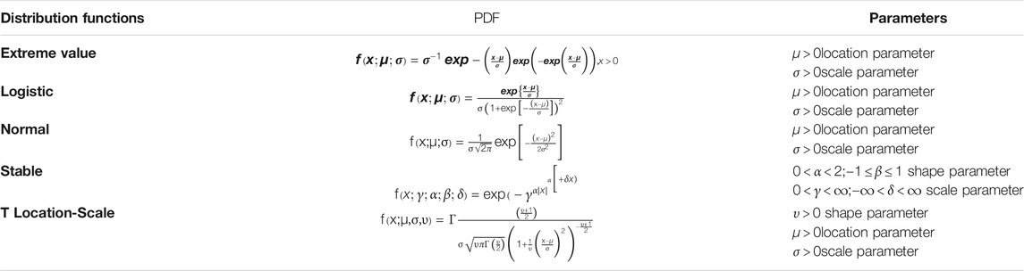
TABLE 1. Probability distribution function (PDF) of the five distribution functions used in the study.

Interval Prediction Theory

Under the significance level $\alpha$, for the limit of the model prediction error interval (I_min and I_max), the probability formula of the prediction model error value ${\widehat{y}}_{err}$ and the prediction error true value $Y_{err}$ can be expressed as follows (Song et al., 2015):

$\mathit{P}\left({\mathit{I}}_{\min }\le {\mathit{Y}}_{err}\le {\mathit{I}}_{\max }\right)=1-2\alpha (39)$

Since the error value of the prediction model is a random variable, Eq. 50 can also be written as follows:

$\mathit{P}\left\{{\mathit{I}}_{\min }\le {\mathit{Y}}_{err}\le {\mathit{I}}_{\max }|\mathit{E}\left(Y_{err}\right)={\widehat{y}}_{err}\right\}=1-2\alpha (40)$

In addition, we assume that the prediction error of the future prediction model has the same distribution function as that of the historical prediction model. Therefore, the probability distribution function (PDF) based on the historical error data of the prediction system can be regarded as a distribution function of future prediction error (Chen and Liu, 2021). Thus, the upper and lower bounds of the function at a certain confidence level can be calculated.

$\left\{\left({\mathit{I}}_{\min },{\mathit{I}}_{\max }\right)|{\mathit{I}}_{\min }\le {\mathit{Y}}_{err}\le {\mathit{I}}_{\max },{\displaystyle \underset{I_{\min }}{\overset{I_{\max }}{\int }}f\left(x|\widehat{\Theta }\right)dx=1-2\alpha }\right\}(41)$

The above equation can also be written as

$\left[{\widehat{\mathit{I}}}_{\min },{\widehat{\mathit{I}}}_{\max }\right]=\left[{\widehat{\mathit{I}}}_{\min },{\widehat{\mathit{y}}}_{err}\right]\begin{array}{c}\\ \end{array}\left[{\widehat{\mathit{y}}}_{err},{\widehat{\mathit{I}}}_{\max }\right](42)$

${\displaystyle \underset{I_{\min }}{\overset{{\widehat{y}}_{err}}{\int }}f\left(x|\widehat{\Theta }\right)}dx=\text{F}\left({\widehat{y}}_{err}\right)-\alpha (43)$

${\displaystyle \underset{{\widehat{y}}_{err}}{\overset{{\hat{I}}_{\max }}{\int }}f\left(x|\widehat{\Theta }\right)}dx=1-\text{F}\left({\widehat{y}}_{err}\right)-\alpha (44)$

After the optimal statistical distribution of the prediction error is determined, the upper $\widehat{U}$and lower $\widehat{L}$ bounds of the carbon price prediction interval can be constructed.

$\left[\widehat{\mathit{L}},\widehat{\mathit{U}}\right]=\left[{\widehat{y}}_{forecast}+{\widehat{I}}_{\min },{\widehat{y}}_{forecast}+{\widehat{I}}_{\max }\right](45)$

In Eq. 45, ${\widehat{y}}_{forecast}$ is the carbon price predicted by the carbon price prediction model.

Ensemble Prediction System and its Interval Forecasting Framework

This section introduces in detail the specific process used in this study. A brief overview of EPS and its uncertainty exploration is shown in Figure 2.

FIGURE 2

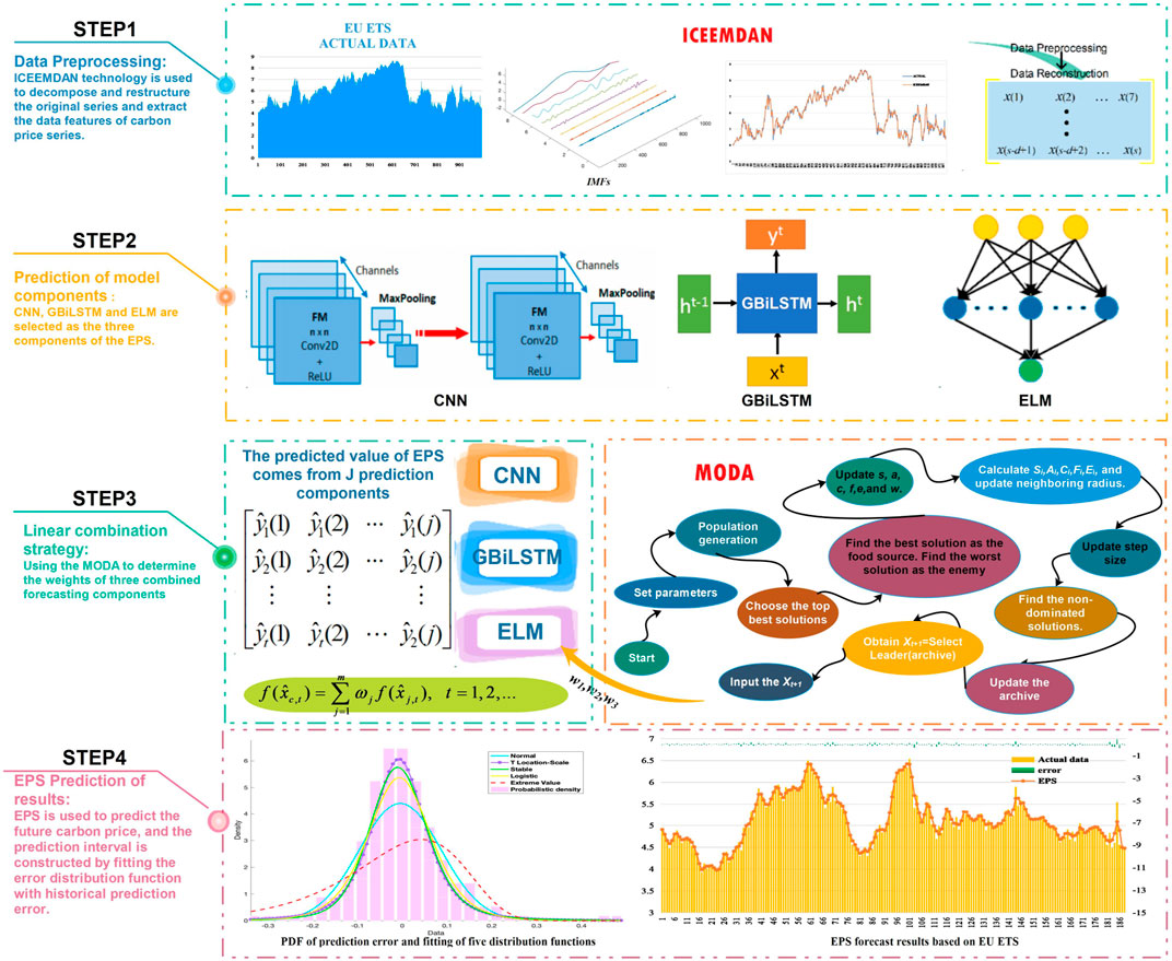
FIGURE 2. EPS system and its interval prediction model framework.

Step 1: Data Preprocessing and Feature Selection Module

In this article, ICEEMDAN technology is employed to decompose and reconstruct the original carbon price data. ICEEMDAN decomposes the original carbon price into several IMFs and residual terms. The IMF with the highest frequency is then eliminated, and the remaining IMFs are reorganized to extract the effective features of the data. For multivariate time series, effective feature selection is also very important. In this study, partial autocorrelation analysis (PACF) is employed to determine the input feature length of carbon price prediction to achieve feature selection.

Step 2: EPS of Model Components

Owing to the high randomness, volatility, and instability of carbon price data, it is not easy to find its rules of motion, and the single hybrid prediction model has inherent defects. Therefore, the use of a combination of hybrid forecasting models is an effective means of obtaining satisfactory prediction performance and improving prediction accuracy. In this study, two deep learning hybrid models (ICEEMDAN-GBiLSTM and ICEEMDAN-CNN) and a feedforward neural network (ICEEMDAN-ELM) are used as the prediction components of the EPS. They have high prediction accuracy and good learning ability for time series.

Step 3: Component Ensemble Strategy

Given the advantages and disadvantages of different hybrid models, it is very important to select a weight combination strategy with strong adaptability and good fusion effect to compensate for the defects of the individual hybrid models and improve the performance and accuracy of carbon price prediction. Therefore, the MODA is selected to determine the fusion weight among the three prediction model components.

Step 4: Exploring Uncertainty

Quantifying the uncertainty associated with carbon price prediction is a considerable challenge. In this study, a new interval prediction scheme based on forecasting error distribution modeling in the model training stage is proposed. Unlike previous research based on the assumption that the prediction error follows a Gaussian distribution, this article uses MLE to conduct statistical research on carbon price error data and to explore its distribution. Among the five DFs developed, the function that best fits the distribution of carbon price prediction error is found. After confirming that the optimal fit to the distribution of forecast error is provided by the t location-scale, the upper and lower bounds of the carbon price prediction interval are constructed based on its PDF.

Experiment and Analysis

This section will introduce the experimental setup and analysis in detail, including the simulation experiment dataset and three different groups of empirical experiments that are used to verify the prediction performance of EPS.

Data Selection and Analysis

In this article, three datasets based on the carbon price market (the EU Emission Trading System (EU ETS), the Shenzhen (SZ), and the Beijing (BJ) datasets) are used as experimental data. The dataset can be downloaded from the wind database (http://www.wind.com.cn/). The first 80% of each dataset is used as the training set, and the last 20% is used as the test set. Specifically, for the EU emission trading system dataset, a total of 1,000 daily quota settlement prices from July 10, 2013 to May 3, 2017 are selected. For the Shenzhen and Beijing datasets, this study used daily spot carbon price data collected from January 14, 2014 to February 7, 2017, including 800 data points. Detailed statistical descriptions of the three datasets are given in Table 2. In addition, in constructing the model input vector, we adopted a rolling acquisition mechanism.

TABLE 2

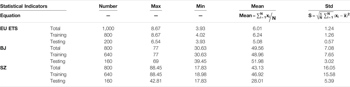
TABLE 2. : Statistical description of the carbon prices reported at three sites.

Model Parameter Setting

The model parameters determine the performance of the prediction system to a large extent. The different parameters of the EPS proposed in this study are obtained by referring to the literature and to the results of the experiments conducted in this study. The parameter settings for each component of the ensemble system are listed in Table 3; this information is valuable and useful because it provides a reference for future research.

TABLE 3

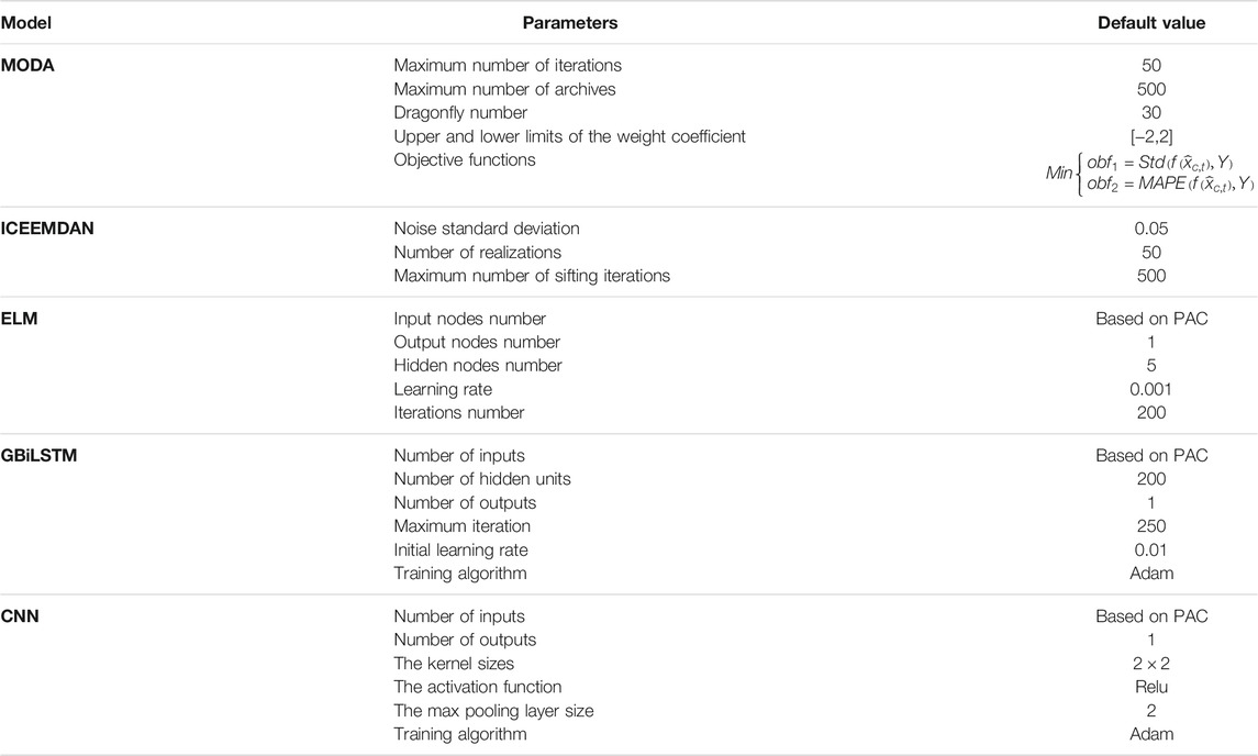
TABLE 3. Model parameters.

Evaluation Index System

To quantify the performance of the developed system, this study constructs an evaluation system using a variety of error evaluation criteria. The system is evaluated and analyzed based on the deterministic point estimation evaluation index and the probabilistic interval estimation evaluation index (Wang R. et al., 2018; Jiang et al., 2021). In the deterministic prediction part, four evaluation indicators, MAE, RMSE, MAPE, and IA, are used. MAE can better express the prediction error under actual conditions. RMSE reflects the deviation between the prediction value and the true value. MAPE expresses the accuracy of prediction using the ratio of error to true value. IA is applied to measure the concordance between the predicted value and the actual value. During interval prediction and evaluation, the three general indicators FICP, FINAW, and AWD are employed to evaluate the quality of the prediction interval. FICP reflects the possibility that the original value falls within the forecast period. FINAW measures the width of the prediction interval. AWD represents the degree of deviation between the observed value and the prediction interval. For FICP, unlike other indicators, a larger value indicates better performance of the model. Table 4 lists the details of the above evaluation indicators.

TABLE 4

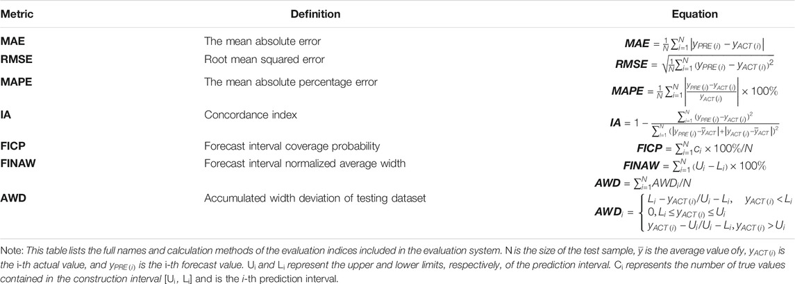
TABLE 4. Basic evaluation metrics.

Experiment 1: Comparison of Different Data Processing Methods

In this experiment, the original carbon price series and the data based on ICEEMDAN, EEMD, and singular spectrum decomposition (SSA) are used as the training input for different prediction models. The purpose of this experiment is to explore the effect of using different signal decomposition techniques on the prediction accuracy of prediction models. Table 6 compares the results obtained using the corresponding models.

Feature Selection Analysis

The prediction performance of both machine learning and deep learning methods is closely related to the input variables. The PACF method is used to select appropriate features as the best input of the prediction model. The best input characteristics obtained from the PACF results of each subsequence are shown in Table 5. (In the follow-up experiments, the input units of each prediction model were obtained according to the PACF results.)

TABLE 5

TABLE 5. Optimal input characteristics based on the PACF.

Prediction Results Obtained Using the Different Data Preprocessing Methods

To verify the effectiveness of the ICEEMDAN data preprocessing method in data feature extraction, in this experiment the performance of ICEEMDAN is compared with that of the classical feature extraction methods EEMD and SSA. The detailed results are described below.

From the results in Table 6, it can be seen that the use of data preprocessing technology can effectively ameliorate the prediction ability of the prediction model. MAPE, MAE, RMSE, and IA were adopted to evaluate the prediction ability of the model based on the prediction accuracy and the fitting situation. For the data on the three carbon trading markets, the MAPE, the MAE, and the RMSE of the prediction model are significantly lower than those of the model that was directly trained on the original dataset, regardless of which data preprocessing technology is adopted. When the original dataset is used directly, the $MAP{E}_{actual}$ of the prediction model under the EU ETS, SZ, and BJ datasets is between 3 and 14%, while the $MAP{E}_{ICEE}$of the prediction model is reduced to 1–5% when ICEEMDAN noise reduction technology is used. This is sufficient to indicate the necessity for data preprocessing.

TABLE 6

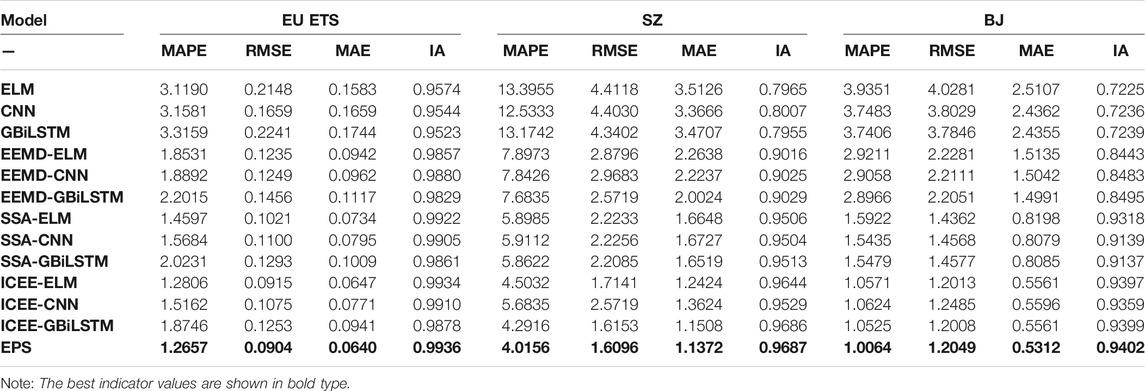
TABLE 6. Comparison of the performances of prediction models based on different data feature extraction techniques.

In addition, for the three components of EPS, different data preprocessing methods are used as model inputs. The experimental results show that ICCEEMDAN is more effective than the other methods. For the EU ETS dataset, the prediction system using ICEEMDAN noise reduction technology has the highest prediction accuracy, and the average RMSE value of the three component models, ${\overline{\mathit{RMSE}}}_{ICEE}^{EUETS}=0.1081$, is the best; the prediction performance of the model based on EEMD is the worst: ${\overline{\mathit{RMSE}}}_{EEMD}^{EUETS}=0.1313$ in the SZ dataset, ${\overline{\mathit{MAE}}}_{ICEE}^{SZ}=1.2518$, ${\overline{\mathit{RMSE}}}_{ICEE}^{SZ}=1.9671$, and ${\overline{\mathit{MAPE}}}_{ICEE}^{SZ}=4.8261\%$. In the BJ dataset, the average values of these three indicators are 0.5573, 1.2169, and 1.0573%, obviously better than those obtained using other data processing technologies.

IA is an effective index that can be used to measure the correlation and consistency between the predicted values and the original data. The higher the index value is, the better the fitting effect of the model is. The ICEEMDAN feature extraction technology proposed in this article achieves the highest IA of all the models tested under the three carbon price datasets. In the SZ dataset, the IA values are $\mathit{I}{\mathit{A}}_{ICEE-ELM}^{SZ}=0.9644$, $\mathit{I}{\mathit{A}}_{ICEE-CNN}^{SZ}=0.9529$, and $\mathit{I}{\mathit{A}}_{ICEE-BiLSTM}^{SZ}=0.9696$. These values are 0.0138, 0.0025, and 0.0173 units higher than ${\text{IA}}_{SSA-ELM}^{SZ}$, $\mathit{I}{\mathit{A}}_{SSA-CNN}^{SZ}$, and $\mathit{I}{\mathit{A}}_{SSA-GBiLSTM}^{SZ}$, respectively, and 0.0628, 0.0504 and 0.0657 units higher than $\mathit{I}{\mathit{A}}_{EEMD-ELM}^{SZ}$, $\mathit{I}{\mathit{A}}_{EEMD-CNN}^{SZ}$和$\mathit{I}{\mathit{A}}_{EEMD-GBiLSTM}^{SZ}$, respectively. In summary, compared with other data preprocessing technologies, ICEEMDAN data preprocessing is more effective for data feature extraction and has incomparable advantages in improving the performance of the prediction model.

Key Finding: Compared with the original carbon price series and other classical data preprocessing techniques, ICEEMDAN preprocessing technology can extract the data characteristics of carbon prices more effectively, significantly enhances the prediction accuracy of the prediction model, and is a more reliable data preprocessing tool.

Experiment 2: Point Forecasting: Comparison of the EPS With Reference Models

To verify the effectiveness of EPS in carbon price prediction, the traditional single forecast model and the classical hybrid prediction model are compared with EPS. These models include the traditional statistical models ARIMA and ICEEMDAN-ARIMA, the traditional single neural network models BP, ELM, GRNN, the deep learning models LSTM, CNN, and the classical hybrid prediction models GWO-BP and ICEEMDAN-GWO-BP. In addition, to explore the expansibility of the model, the experimental content of multistep point prediction is included in the experiment. In the multistep prediction, rolling prediction is adopted. The specific method used to perform multistep prediction is shown in Figure 3. The experimental results are shown in Table 7. The detailed experimental analysis is described below.

1) In comparison with the traditional single prediction model, we find that EPS displays incomparable advantages in the four indicators in both one-step and multiple-step prediction. This shows that the EPS developed by us is effective in predicting carbon prices. In addition, the MAPE values of GBiLSTM in the three datasets are $MAP{E}_{GB\text{i}LSTM}^{EUETS}=3.3159$, $MAP{E}_{GB\text{i}LSTM}^{SZ}=13.1740$, and $MAP{E}_{GB\text{i}LSTM}^{BJ}=3.7406$; these values are better than those obtained using a single LSTM, proving the effectiveness of the GBiLSTM. The other two prediction components, ELM and CNN, have outstanding prediction performance in all single prediction models, so it is reasonable to choose them as the submodes of the EPS. In addition, we can see that for the traditional statistical model ARIMA, the average value of MAPE of the three stations is ${\overline{\mathrm{MAPE}}}_{ARIMA}=11.0072$in one-step prediction; this is not as high as the prediction accuracy achieved using other prediction models, indicating that the traditional linear statistical model is not suitable for the prediction of carbon price series with high volatility and complexity.

2) We can observe that under different datasets, different prediction models have different prediction performances. Under the EU ETS dataset, the neural network ELM performs best, yielding $RMS{E}_{ELM}^{EUETS}=0.2148$; this is better than the RMSE values of the deep learning algorithms CNN and GBiLSTM, which are $RMS{E}_{CNN}^{EUETS}=0.2218$ and $RMS{E}_{BiLSTM}^{EUETS}=0.2241$, respectively. However, under the SZ and BJ datasets, the deep learning algorithms CNN and GBiLSTM achieve better prediction results than ELM. The same phenomenon occurs in multistep forecasting, and there the forecast advantage of the deep learning framework is more obvious. However, the prediction accuracy of EPS remains the highest under any of the tested datasets. The RMSE values in the one-step forecast are $RMS{E}_{EPS}^{EUETS}=0.0904$, $RMS{E}_{EPS}^{SZ}=1.6096$, and $RMS{E}_{EPS}^{BJ}=1.2046$. The RMSE values in the two-step forecast are $RMS{E}_{EPS}^{EUETS}=0.1829$, $RMS{E}_{EPS}^{SZ}=3.3244$, and $RMS{E}_{EPS}^{BJ}=1.7567$. This shows that the combination strategy retains the forecasting advantages obtained by using different forecasting components and that it compensates for each model’s defects; as a result, EPS has strong robustness and wide adaptability.

FIGURE 3

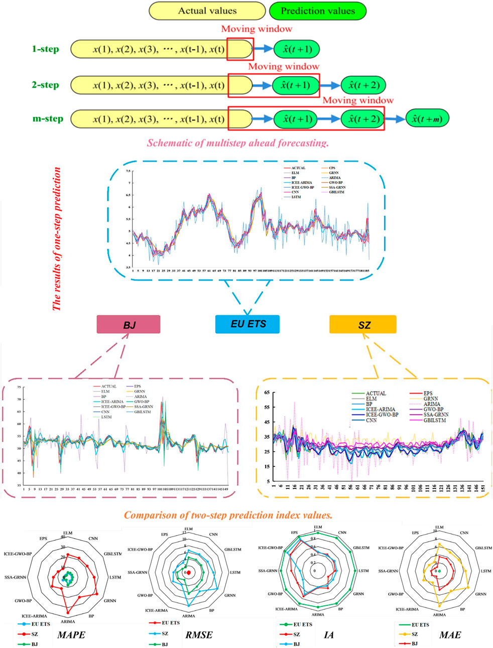
FIGURE 3. Prediction results obtained using EPS and comparison models under different prediction steps.

TABLE 7

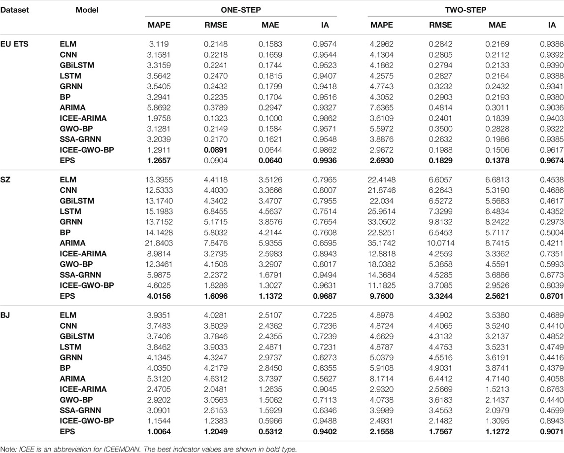
TABLE 7. Comparison of the prediction ability of the proposed system with those of some traditional benchmark models and classic hybrid models.

In comparison with the classic hybrid forecasting models ICEE-GWO-BP, SSA-GRNN, and GWO-BP, several sets of hybrid forecasting methods have achieved good forecasting performance; however, because the index values used in these models are very similar, it is not easy to intuitively present the predictive ability of the model. In this case, we measure the percentage of improvement in the evaluation index to make the analysis more intuitive. The percentage of improvement in the evaluation index is a measure of the degree of improvement achieved by EPS compared with the index value of the comparison model; it can be expressed as follows:

${\mathit{P}}_{Index}^{model}=\left|\frac{\mathit{Inde}{\mathit{x}}_{model}-\mathit{Inde}{\mathit{x}}_{EPS}}{\mathit{Inde}{\mathit{x}}_{model}}\right|\times 100\%(46)$

where${\text{P}}_{Index}^{model}$is the percentage of improvement indicators, ${\text{Index}}_{model}$ stands for the index value of the comparison model, and ${\text{Index}}_{EPS}$is the index value of the EPS.

In the EU ETS dataset, the improved MAPE values for one-step prediction of the three hybrid models are $P_{MAPE}^{ICEE-GWO-BP}=1.9673\%$, $P_{MAPE}^{SSA-GRNN}=60.4950\%$, and $P_{MAPE}^{GWO-BP}=59.5377\%$. The improved MAPE values of the two-step prediction are $P_{MAPE}^{ICEE-GWO-BP}=9.2410\%$, $P_{MAPE}^{SSA-GRNN}=30.7285\%$ and $P_{MAPE}^{GWO-BP}=51.8867\%$. Under the BJ dataset, the improved IA values predicted for the three hybrid models using the one-step method are $P_{IA}^{ICEE-GWO-BP}=0.9064\%$, $P_{IA}^{SSA-GRNN}=48.1563\%$, and $P_{IA}^{GWO-BP}=33.3896\%$. The improved IA values obtained by two-step prediction are $P_{MAPE}^{ICEE-GWO-BP}=1.4313\%$, $P_{MAPE}^{SSA-GRNN}=97.2385\%$, and $P_{MAPE}^{GWO-BP}=104.3018\%$. The index improvement percentage more intuitively shows the improvement in prediction performance obtained using EPS. Compared with the classical hybrid prediction model, the EPS shows significant improvement in both prediction accuracy and fitting consistency.

Figure 3 shows a comparison of the prediction results obtained using EPS and the comparison model when different numbers of prediction steps are used.

Key finding: The difference in the prediction results between the EPS system and other prediction models is significant. Specifically, under each dataset and for each prediction step, the EPS has better prediction performance. Therefore, it is concluded that the advanced ensemble prediction system has better carbon price forecasting ability and potential than the traditional single models and classical hybrid models.

Experiment 3: Interval Forecasting: Uncertainty Analysis of Carbon Price

In Experiment 2, the accuracy and stability of the prediction system were discussed through the prediction method of certainty point estimation. However, the point prediction results do not reflect the uncertainty in the dataset. To further prove that the ESP system has a wider range of adaptability than other predictive models, this section uses the interval prediction method to mine the uncertainty of carbon prices. Unlike point prediction, interval prediction can provide the upper and lower bounds of the observed value, making it possible to construct the prediction interval under a given significance level. It can provide additional information for carbon price market policymakers and can help them analyze the carbon price market.

Distribution Function of Prediction Error

In previous studies, most of the prediction errors of the prediction model defaulted to obey the normal distribution. However, the normal distribution function does not effectively reflect the distribution of forecast model errors. Therefore, this research develops five fitting distribution functions and uses the MLE method to conduct an in-depth investigation of the prediction error to obtain a distribution function (DF) with better fitting performance. The most suitable probability distribution for further interval prediction is selected.

In this section, five DFs, namely, extreme value, normal, logistic, stable, and t location-scale, are used to represent the distribution of carbon price prediction errors. Table 1 shows the relative PDF of these DFs. Table 8 lists the five DF parameters estimated by the MLE method. These parameters can be used to describe the scale and location of these DFs. In addition, the coefficient of determination (0 ≤ R² ≤ 1) and RMSE are used to determine the degree of fit of these DFs. The larger the R² value is, the lower the RMSE value is, and the better is the fitting ability of the DFs. The index values reflecting the fitting abilities of the five DFs are shown in Table 9 and Figure 4.

TABLE 8

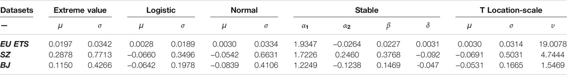
TABLE 8. Parameter values of the different distribution functions determined by MLE.

TABLE 9

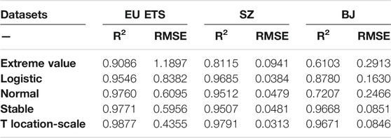
TABLE 9. R² and RMSE values of the five distribution functions by MLE.

FIGURE 4

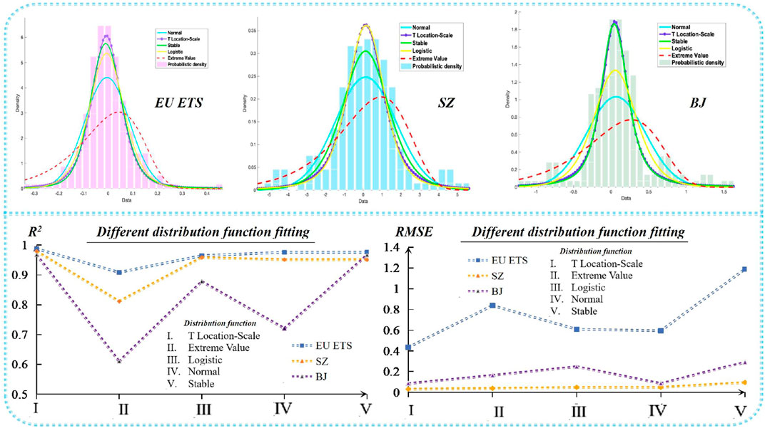
FIGURE 4. Five distribution functions fit the distribution of EPS error.

Table 9 shows that the t location-scale function fits the EPS prediction error best. Its R² value is higher than 0.96, and its RMSE value is the lowest, indicating that it can provide better estimates in all cases, followed by stable distribution, normal distribution, logistic distribution, and extreme value distribution. In addition, although the stable distribution has a slightly worse fitting effect than the t location-scale distribution, it is still better than the normal distribution that the previous prediction error hypothesis obeys; this further proves the necessity of fitting the distribution of the prediction error. In addition, the motivation for estimating the distribution function of the carbon price dataset in this section is to prepare for further research on the establishment of carbon price interval predictions, as discussed in Section Interval Prediction of Carbon Price.

Interval Prediction of Carbon Price

Unlike the deterministic information given by the point forecast, the interval forecast can provide the forecast range, a confidence level, and other uncertain information on future values; this information is helpful to decision-makers who are attempting to analyze and supervise the reasonable operation of the carbon price market. Owing to the generalization ability of the forecasting model, the complex patterns of carbon price series fluctuations and other factors inevitably produce forecast errors, and the ability to effectively transform the uncertainty caused by forecast errors into measurable features is of great significance. Therefore, in this study, a new interval prediction scheme based on modeling of the prediction error distribution in the model training phase is proposed.

According to the point prediction results of the proposed EPS system, the t location-scale distribution function, which determines the prediction error in Section Distribution Function of Prediction Error, and the interval prediction method introduced in Section Interval Prediction Theory, the prediction interval is constructed under the given significance level α. To verify that the prediction interval constructed by the t location-scale model has the best fit, it is compared with the other four error distribution functions.

In addition, three evaluation indicators, FINAW, PICP, and AWD, listed in Table 4, are introduced in this section to present the effect of interval prediction. It is worth mentioning that the optimal interval prediction should satisfy the following conditions: under a given significance level $\alpha$, the larger the PICP value is (0 ≤ PICP ≤ 1), the smaller the FINAW value is, and the better is the prediction performance of interval prediction. However, it is obvious that there is a contradiction between FINAW and PICP. When the PICP value increases, the FINAW of the response average bandwidth will certainly increase. Therefore, the AWD index is introduced as a supplement to the evaluation index system. Table 10 shows the prediction intervals of the EPS system as evaluated based on the three carbon price markets using five different error distributions.

TABLE 10

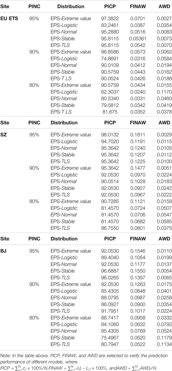
TABLE 10. Carbon price range prediction results based on EU ETS, SZ, and BJ under different significance levels.

In theory, when the PICP is greater than the significance level, the constructed prediction interval is effective. As seen from Table 10, the models satisfying this condition are EPS-TLS and EPS-Extreme value; these models are effective at the 95, 90, and 80% significance levels. However, if the value of the PICP is the only goal, the result will become meaningless, as increased PICP inevitably leads to a larger FINAW. Based on different $\alpha$conditions, the value of $FINA{W}_{EPS-Extremevalue}$is significantly higher than the FINAW value obtained through modeling of other distributions. At the same time, considering that in Section Distribution Function of Prediction Error, the fitting of extreme value distribution to EPS prediction error is very bad, it can be considered that the prediction interval constructed by EPS-Extreme value is not reasonable.

The PICP of EPS-TLS in the data from the three carbon trading markets is higher than the significance level$\alpha$. In addition, under different$\alpha$, the FINAW values of the three markets are $FINA{W}_{EPS-TLS}^{EUETS}=0.0542$, $FINA{W}_{EPS-TLS}^{SZ}=0.1225$, and $FINA{W}_{EPS-TLS}^{BJ}=0.1397$. The FINAW value is not optimal in any of the five interval prediction models, but with only a small increase in the FINAW value, the other index values achieve better results. All things considered, this can be accepted.

For the prediction interval constructed using a normal distribution, in the BJ dataset, the PICP values of EPS-Normal are $PIC{P}_{EPS-Normal}^{BJ}=92.0530$ and $PIC{P}_{EPS-Normal}^{BJ}=88.0795$ under significance levels of 0.95 and 0.90, respectively; they fail to meet the condition of a level of $\alpha$ that is greater than significance. This also reflects the necessity of detailed research on error distribution. For AWD indicators, although $AW{D}_{EPS-TLS}$ is not all better than the benchmark model, there is little difference. Considering the comprehensive performance of the three indicators of the proposed scenario, EPS-TLS still has obvious advantages over the four benchmark models in constructing the prediction interval.

In addition, the carbon price prediction intervals generated by the three proposed schemes of the three carbon trading markets are shown in Figure 5. It can be observed that EPS-TLS has a smaller bandwidth and is surrounded by these constructed prediction intervals in most target values. The constructed confidence interval is very effective.

FIGURE 5

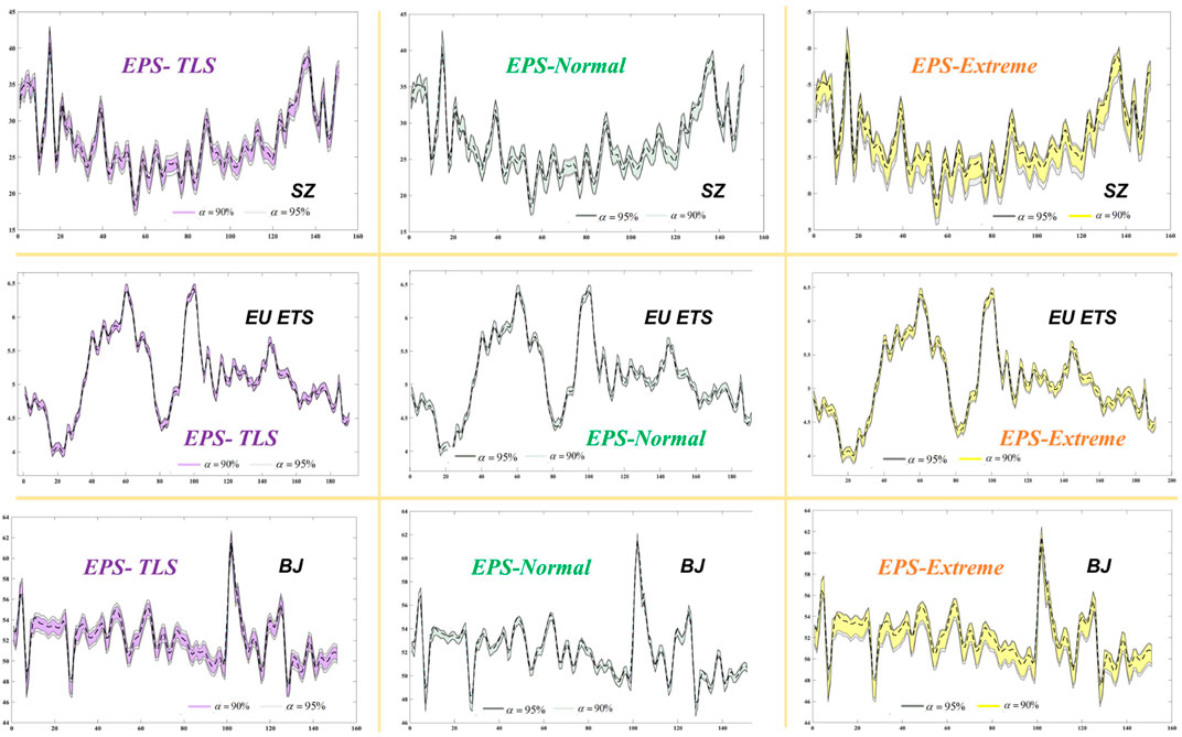
FIGURE 5. Carbon price prediction intervals generated by the three proposed schemes.

Discussion

In this section, we will discuss the robustness, application, and further development of EPS in the carbon price market.

Robustness Discussion

Because the results of both deep learning and metaheuristic optimization algorithms are always accompanied by randomness and probability mechanisms, the results of each experiment will still have deviations even when the parameters are set exactly the same. At the same time, in the actual forecast, the actual values of the future carbon price cannot be predicted in advance; thus, it is impossible to use the evaluation index to verify the future value in advance. Therefore, the stability of the EPS is also an important factor that affects the prediction.

The standard deviation is an effective measure of system stability. It can be indicated as ${\mathrm{SD}}_{\left(M\right)}=\sqrt{{\displaystyle {\sum }_k^n{\left(M_k-\overline{M}\right)}^2/n}}$, where n is the number of training iterations, M_K is the predicted value of the K-th training result, and M is the average of the N-th results (Xiao et al., 2017). The smaller the value of SD, the higher the stability of the model.

To evaluate the stability of the different models, the SD_(M) values of four evaluation indices were calculated in 30 prediction experiments using three carbon price datasets.

Table 11 shows a comparison of the stability test results of different prediction systems based on ICEEMDAN processing. In the EU ETS dataset, ICEE-ELM has good stability ($S{D}_{\left(MAPE\right)}^{ICEE-ELM}=0.0105$), but the stability is still slightly lower than that of the EPS prediction system ($S{D}_{\left(MAPE\right)}^{EPS}=0.0101$). In the BJ and SZ datasets, CNN has good prediction accuracy in previous experiments, but its robustness is not good, and the prediction results fluctuate greatly. In contrast, EPS obtains a smaller SD value regardless of which dataset is used. This further shows that different single prediction systems have different robustness when used with different datasets and indicates that EPS with a combination weighting strategy can be considered the prediction method that obtains the best prediction results.

TABLE 11

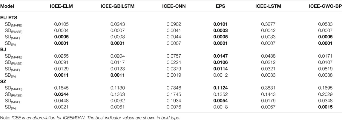
TABLE 11. Certainty of different forecasting methods.

It is worth mentioning that the average prediction stability of GBiLSTM in the three prediction datasets is better than that of the traditional LSTM model; that is,$\overline{S{D}_{\left(RMSE\right)}^{\mathrm{GBiLSTM}}}=0.0496$, but $\overline{S{D}_{\left(RMSE\right)}^{LSTM}}=0.0566$. The results show that the proposed GBiLSTM not only has better prediction accuracy than LSTM but also that its robustness is significantly improved.

Application of the Proposed Ensemble Prediction System

1) A stable carbon price prediction system plays a prominent role in the initial allocation of the carbon quota, in transaction pricing and in effective monitoring of market risk. The proposed EPS system not only shows accurate point prediction performance but also reasonably analyzes and mines the potential uncertainty of carbon prices by constructing the carbon price prediction interval based on error distribution fitting.

2) The proposed EPS system combines a deep learning framework with a traditional neural network and thereby provides a new idea for carbon price prediction and an effective reference tool that policymakers can use to research the volatility of the carbon market.

3) Comparing the EU ETS market data with the carbon price markets in Shenzhen and Beijing, it is helpful for China to analyze the evolution of the mature carbon trading market price in the EU; this will help the regulatory authorities adjust the policy and ensure the steady development of China’s carbon market.

4) EPS has high practical value and strong expansibility and can easily fit highly volatile nonlinear time series. It thus provides a new intelligent supervision scheme for building a sound global carbon trading market in the future. At the same time, the use of a deep learning integrated forecasting system with high accuracy and strong stability is expected to become a new direction of energy and financial markets in the future.

Suggestions on Further Improvement of Carbon Price Market

More accurate prediction of carbon prices can provide some effective suggestions through which governments and enterprises can build and improve the carbon price market in the future. These are outlined below.

Improvement of the Initial Allocation Mechanism of Carbon Emission Rights

In the initial allocation of carbon quotas, we should pay attention to the fairness of allocation. First, the government should formulate incentive policies to encourage regional governments and local enterprises to reduce emissions and should give appropriate incentives or policy support to the regions and enterprises that use emission reduction technologies. Second, the initial allocation of carbon emission rights requires effective operation and an effective regulatory system; both of these components directly affect the efficiency and fairness of carbon quota allocation. Strengthening the construction of a carbon emission rights regulatory system will help achieve efficiency and fairness of resource allocation as China’s total emission reduction target is being met.

Rationalization of the Carbon Trading Pricing System

Owing to the imperfect development of the carbon trading market and the carbon trading pricing system, the carbon trading price is easily affected by monopoly enterprises. At present, there is a certain monopoly phenomenon in the carbon trading market in some regions of China. Some small buyer enterprises can only passively accept the carbon price, and this allows monopoly enterprises to disproportionately influence the supply and demand of the market and reduces total social welfare. The establishment of a reasonable pricing system that avoids monopoly price manipulation is conducive to the return of carbon prices to real value levels and to the optimal allocation of resources.

Improvement of the Carbon Market Risk Management and Control System

In the process of price fluctuation risk control, an accurate and effective price forecasting model can be used to monitor price fluctuations. Using the relevant data, such a model can be used to predict long-term and short-term carbon trading prices, predict future fluctuation trends, and establish an effective carbon trading price risk early warning index system to effectively monitor the volatility risk caused by market price fluctuations. Through prediction of the carbon trading market price, we can grasp the fluctuations in carbon prices and take measures in advance to exercise macro control and reduce the level of risk when large market price fluctuations occur.

Conclusion

The availability of a reliable carbon price forecasting system is significant in the emission trading market because it can help decision-makers evaluate climate policies and adjust the emission ceiling to effectively maintain the reliable operation of the market. In this study, the EPS system, which adopts advanced data feature extraction and selection methods, combines the three optimal submodels through a multiobjective dragonfly optimization algorithm and explores the deterministic and uncertainty prediction of carbon price series. This study has several important implications: 1) ICEEMDAN is better than traditional signal decomposition at extracting data features. This can improve the accuracy of the prediction system. 2) The deep learning algorithm has a better ability than other algorithms to forecast carbon price series. The developed GBiLSTM model has better predicted performance and stability than the traditional LSTM. 3) Unlike previous studies in which it was assumed that the prediction error obeys a Gaussian distribution, this study explores five fitting distribution functions of prediction error, finds a more accurate error distribution function, and constructs a more reasonable carbon price prediction interval. The experimental results indicate that the EPS prediction system achieves the best prediction performance, with MAPE values of 1.2657, 4.0156, and 1.0064% for the three datasets. In addition, according to the optimal distribution fitting function of EPS prediction error, the carbon price prediction interval is constructed to mine the uncertainty of carbon price fluctuation. At various significance levels, the constructed prediction interval contains most of the observations, showing that the interval prediction has good performance. Therefore, the system is an effective supplement to the existing carbon price prediction research framework and contributes to the ability of the government to reduce market risk and stabilize the market.

Although the combined prediction system proposed in this article achieves good prediction performance, there are still some limitations due to practical factors. Future research will analyze the carbon price trend from two perspectives, historical carbon price series and external factors, to obtain more accurate and stable prediction results.

Data Availability Statement

The original contributions presented in the study are included in the article/Supplementary Material, further inquiries can be directed to the corresponding author.

Author Contributions

YY: Conceptualization, Methodology. HG: Writing-Reviewing and Editing, Data curation. YJ: Formal analysis, Supervision. AS: Software, Validation and Visualization, Investigation.

Funding

This work was supported by the Major Project of the National Social Science Fund (Grant No. 17ZDA093).

Conflict of Interest

The authors declare that the research was conducted in the absence of any commercial or financial relationships that could be construed as a potential conflict of interest.

Publisher’s Note

All claims expressed in this article are solely those of the authors and do not necessarily represent those of their affiliated organizations, or those of the publisher, the editors and the reviewers. Any product that may be evaluated in this article, or claim that may be made by its manufacturer, is not guaranteed or endorsed by the publisher.

References

Arouri, M. E. H., Jawadi, F., and Nguyen, D. K. (2012). Nonlinearities in Carbon Spot-Futures price Relationships during Phase II of the EU ETS. Econ. Model. 29 (3), 884–892. doi:10.1016/j.econmod.2011.11.003

CrossRef Full Text | Google Scholar

Atsalakis, G. S. (2016). Using Computational Intelligence to Forecast Carbon Prices. Appl. Soft Comput. 43, 107–116. doi:10.1016/j.asoc.2016.02.029

CrossRef Full Text | Google Scholar

Benz, E. A., and Trück, S. (2009). Modeling the price Dynamics of CO2 Emission Allowances. Energ. Econ. 31, 4–15. doi:10.1016/j.eneco.2008.07.003

CrossRef Full Text | Google Scholar

Byun, S. J., and Cho, H. (2013). Forecasting Carbon Futures Volatility Using GARCH Models with Energy Volatilities. Energ. Econ. 40, 207–221. doi:10.1016/j.eneco.2013.06.017

CrossRef Full Text | Google Scholar

Chen, C., and Liu, H. (2021). Dynamic Ensemble Wind Speed Prediction Model Based on Hybrid Deep Reinforcement Learning. Adv. Eng. Inform. 48, 101290. doi:10.1016/J.AEI.2021.101290

CrossRef Full Text | Google Scholar

Cheng, Z., and Wang, J. (2020). A New Combined Model Based on Multi-Objective Salp Swarm Optimization for Wind Speed Forecasting. Appl. Soft Comput. 92, 106294. doi:10.1016/j.asoc.2020.106294

CrossRef Full Text | Google Scholar

Chevallier, J. (2009). Carbon Futures and Macroeconomic Risk Factors: A View from the EU ETS. Energ. Econ. 31 (4), 614–625. doi:10.1016/j.eneco.2009.02.008

CrossRef Full Text | Google Scholar

Chung, J., Gulcehre, C., Cho, K., and Bengio, Y. (2014). “Empirical Evaluation of Gated Recurrent Neural Networks on Sequence Modeling,” in NIPS 2014 Workshop on Deep Learning. ArXiv e-prints Available at: https://arxiv.org/abs/1412.3555.

Google Scholar

Colominas, M. A., Schlotthauer, G., and Torres, M. E. (2014). Improved Complete Ensemble EMD: a Suitable Tool for Biomedical Signal Processing. Biomed. Signal Process. Control. 14, 19–29. doi:10.1016/j.bspc.2014.06.009

CrossRef Full Text | Google Scholar

Du, P., Wang, J., Yang, W., and Niu, T. (2020). Point and Interval Forecasting for Metal Prices Based on Variational Mode Decomposition and an Optimized Outlier-Robust Extreme Learning Machine. Resour. Pol. 69, 101881. doi:10.1016/J.RESOURPOL.2020.101881

CrossRef Full Text | Google Scholar

Fan, X., Li, S., and Tian, L. (2015). Chaotic Characteristic Identification for Carbon price and an Multi-Layer Perceptron Network Prediction Model. Expert Syst. Appl. 42 (8), 3945–3952. doi:10.1016/j.eswa.2014.12.047

CrossRef Full Text | Google Scholar

Hochreiter, S., and Schmidhuber, J. (1997). Long Short-Term Memory. Neural Comput. 9, 1735–1780. doi:10.1162/neco.1997.9.8.1735

PubMed Abstract | CrossRef Full Text | Google Scholar

Huang, G-B., Zhu, Q-Y., and Siew, C-K. (2006). Extreme Learning Machine: Theory and Applications. Neurocomputing 1. doi:10.1016/j.neucom.2005.12.126

CrossRef Full Text | Google Scholar

Jiang, H., Tao, C., Dong, Y., and Xiong, R. (2020). Robust Low-Rank Multiple Kernel Learning with Compound Regularization. Eur. J. Oper. Res. 295, 634–647. doi:10.1016/J.EJOR.2020.12.024

CrossRef Full Text | Google Scholar

Jiang, H., Luo, S., and Dong, Y. (2021a). Simultaneous Feature Selection and Clustering Based on Square Root Optimization. Eur. J. Oper. Res. 289, 214–231. doi:10.1016/j.ejor.2020.06.045

CrossRef Full Text | Google Scholar

Jiang, H., Zheng, W., and Dong, Y. (2021b). Sparse and Robust Estimation with ridge Minimax Concave Penalty. Inf. Sci. 571, 154–174. doi:10.1016/J.INS.2021.04.047

CrossRef Full Text | Google Scholar

Jiang, P., Liu, Z., Niu, X., and Zhang, L. (2021). A Combined Forecasting System Based on Statistical Method, Artificial Neural Networks, and Deep Learning Methods for Short-Term Wind Speed Forecasting. Energy 217, 119361. doi:10.1016/J.ENERGY.2020.119361

CrossRef Full Text | Google Scholar

Jin, Y., Guo, H., Wang, J., and Song, A. (2020). A Hybrid System Based on LSTM for Short-Term Power Load Forecasting. Energies 13 (23), 6241. doi:10.3390/en13236241

CrossRef Full Text | Google Scholar

Liu, Z., Jiang, P., Zhang, L., and Niu, X. (2020). A Combined Forecasting Model for Time Series: Application to Short-Term Wind Speed Forecasting. Appl. Energ. 259, 114137. doi:10.1016/j.apenergy.2019.114137

CrossRef Full Text | Google Scholar

Liu, Z., Jiang, P., Wang, J., and Zhang, L. (2021). Ensemble Forecasting System for Short-Term Wind Speed Forecasting Based on Optimal Sub-model Selection and Multi-Objective Version of Mayfly Optimization Algorithm. Expert Syst. Appl. 177, 114974. doi:10.1016/J.ESWA.2021.114974

CrossRef Full Text | Google Scholar

Lu, H., Ma, X., Huang, K., and Azimi, M. (2020). Carbon Trading Volume and price Forecasting in China Using Multiple Machine Learning Models. J. Clean. Prod. 249, 119386. doi:10.1016/j.jclepro.2019.119386

CrossRef Full Text | Google Scholar

Mirjalili, S. (2016). Dragonfly Algorithm: a New Meta-Heuristic Optimization Technique for Solving Single-Objective, Discrete, and Multi-Objective Problems. Neural Comput. Applic 27, 1053–1073. doi:10.1007/s00521-015-1920-1

CrossRef Full Text | Google Scholar

Niu, T., Wang, J., Lu, H., Yang, W., and Du, P. (2020). Developing a Deep Learning Framework with Two-Stage Feature Selection for Multivariate Financial Time Series Forecasting. Expert Syst. Appl. 148, 113237. doi:10.1016/j.eswa.2020.113237

CrossRef Full Text | Google Scholar

Shi, X., Chen, Z., Wang, H., Yeung, D. Y., Wong, W. K., and Woo, W. C. (2015). “Convolutional LSTM Network: A Machine Learning Approach for Precipitation Nowcasting,” in Advances in Neural Information Processing Systems (NIPS 2015). ArXiv e-prints Available at: https://arxiv.org/abs/1506.04214.

Google Scholar

Song, J., and Li, S. (2017). Elite Opposition Learning and Exponential Function Steps-Based Dragonfly Algorithm for Global Optimization. IEEE Int. Conf. Inf. Autom. ICIA. doi:10.1109/ICInfA.2017.8079080

CrossRef Full Text | Google Scholar

Song, Y., Qin, S., Qu, J., and Liu, F. (2015). The Forecasting Research of Early Warning Systems for Atmospheric Pollutants: A Case in Yangtze River Delta Region. Atmos. Environ. 118, 58–69. doi:10.1016/j.atmosenv.2015.06.032

CrossRef Full Text | Google Scholar

Sun, Y., Wang, X., Chen, Y., and Liu, Z. (2018). A Modified Whale Optimization Algorithm for Large-Scale Global Optimization Problems. Expert Syst. Appl. doi:10.1016/j.eswa.2018.08.027

CrossRef Full Text | Google Scholar

Tian, C., and Hao, Y. (2020). Point and Interval Forecasting for Carbon price Based on an Improved Analysis-Forecast System. Appl. Math. Modelling(C). doi:10.1016/j.apm.2019.10.022

CrossRef Full Text | Google Scholar

Torres, M. E., Colominas, M. A., Schlotthauer, G., and Flandrin, P. (2011). “A Complete Ensemble Empirical Mode Decomposition with Adaptive Noise,” in ICASSP, IEEE International Conference on Acoustics, Speech and signal processing- Proceedings, 4144e7. doi:10.1109/ICASSP.2011.5947265

CrossRef Full Text | Google Scholar

Wang, J., Niu, T., Du, P., and Yang, W. (2020). Ensemble Probabilistic Prediction Approach for Modeling Uncertainty in Crude Oil price. Appl. Soft Comput. 95, 106509. doi:10.1016/j.asoc.2020.106509

CrossRef Full Text | Google Scholar

Wang, J., Niu, X., Zhang, L., and Lv, M. (2021). Point and Interval Prediction for Non-ferrous Metals Based on a Hybrid Prediction Framework. Resour. Pol. 73, 102222. doi:10.1016/J.RESOURPOL.2021.102222

CrossRef Full Text | Google Scholar

Wang, R., Li, J., Wang, J., and Gao, C. (2018). Research and Application of a Hybrid Wind Energy Forecasting System Based on Data Processing and an Optimized Extreme Learning Machine [J]. Energies 11, 1712. doi:10.3390/en11071712

CrossRef Full Text | Google Scholar

Wang, Y., Zhang, N., Tan, Y., Hong, T., Kirschen, D. S., and Kang, C. (2019). Combining Probabilistic Load Forecasts. IEEE Trans. Smart Grid 10, 3664–3674. doi:10.1109/TSG.2018.2833869

CrossRef Full Text | Google Scholar

Wang, G. (2018). Design of Damage Identification Algorithm for Mechanical Structures Based on Convolutional Neural Network. Concurrency Computat Pract. Exper 30, e4891. doi:10.1002/cpe.4891

CrossRef Full Text | Google Scholar

Wang, J. (2020). OCT Image Recognition of Cardiovascular Vulnerable Plaque Based on CNN. IEEE Access 8, 140767–140776. doi:10.1109/access.2020.3007599

CrossRef Full Text | Google Scholar

Wei, S., Chongchong, Z., and Cuiping, S. (2018). Carbon Pricing Prediction Based on Wavelet Transform and K-ELM Optimized by Bat Optimization Algorithm in China ETS: the Case of Shanghai and Hubei Carbon Markets. Carbon Manage. 9 (6), 605–617. doi:10.1080/17583004.2018.1522095

CrossRef Full Text | Google Scholar

Xiao, L., Qian, F., and Shao, W. (2017). Multi-step Wind Speed Forecasting Based on a Hybrid Forecasting Architecture and an Improved Bat Algorithm. Energ. Convers. Manage. 143, 410–430. doi:10.1016/j.enconman.2017.04.012

CrossRef Full Text | Google Scholar

Zhang, X., Wang, J., and Zhang, K. (2017). Short-term Electric Load Forecasting Based on Singular Spectrum Analysis and Support Vector Machine Optimized by Cuckoo Search Algorithm. Electric Power Syst. Res. 146, 270–285. doi:10.1016/j.epsr.2017.01.035

CrossRef Full Text | Google Scholar

Zhang, X., and Wang, J. (2018). A Novel Decomposition‐ensemble Model for Forecasting Short‐term Load‐time Series with Multiple Seasonal Patterns. Soft Comput. 65, 478–494. doi:10.1016/j.asoc.2018.01.017

CrossRef Full Text | Google Scholar

Zhu, B., and Wei, Y. (2013). Carbon price Forecasting with a Novel Hybrid ARIMA and Least Squares Support Vector Machines Methodology. Omega 41, 517–524. doi:10.1016/j.omega.2012.06.005

CrossRef Full Text | Google Scholar

Zhu, B., Yuan, L., and Ye, S. (2019). Examining the Multi-Timescales of European Carbon Market with Grey Relational Analysis and Empirical Mode Decomposition. Physica A: Stat. Mech. its Appl. 517, 392–399. doi:10.1016/j.physa.2018.11.016

CrossRef Full Text | Google Scholar

Zhu, J., Wu, P., Chen, H., Liu, J., and Zhou, L. (2019). Carbon price Forecasting with Variational Mode Decomposition and Optimal Combined Model. Physica A: Stat. Mech. its Appl. 519, 140–158. doi:10.1016/j.physa.2018.12.017

CrossRef Full Text | Google Scholar

Appendix

APPENDIX A1

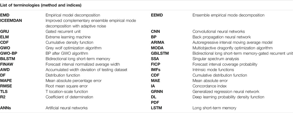
APPENDIX A1. The list of abbreviations in this study.