Abstract
Optical remote sensing has been suggested as a preferred method for monitoring submerged aquatic vegetation (SAV), a critical component of freshwater ecosystems that is facing increasing pressures due to climate change and human disturbance. However, due to the limited prior application of remote sensing to mapping freshwater vegetation, major foundational knowledge gaps remain, specifically in terms of the specificity of the targets and the scales at which they can be monitored. The spectral separability of SAV from the St. Lawrence River, Ontario, Canada, was therefore examined at the leaf level (i.e., spectroradiometer) as well as at coarser spectral resolutions simulating airborne and satellite sensors commonly used in the SAV mapping literature. On a Leave-one-out Nearest Neighbor criterion (LNN) scale of values from 0 (inseparable) to 1 (entirely separable), an LNN criterion value between 0.82 (separating amongst all species) and 1 (separating between vegetation and non-vegetation) was achieved for samples collected in the peak-growing season from the leaf level spectroradiometer data. In contrast, samples from the late-growing season and those resampled to coarser spectral resolutions were less separable (e.g., inter-specific LNN reduction of 0.25 in late-growing season samples as compared to the peak-growing season, and of 0.28 after resampling to the spectral response of Landsat TM5). The same SAV species were also mapped from actual airborne hyperspectral imagery using target detection analyses to illustrate how theoretical fine-scale separability translates to an in situ, moderate-spatial scale application. Novel radiometric correction, georeferencing, and water column compensation methods were applied to optimize the imagery analyzed. The SAV was generally well detected (overall recall of 88% and 94% detecting individual vegetation classes and vegetation/non-vegetation, respectively). In comparison, underwater photographs manually interpreted by a group of experts (i.e., a conventional SAV survey method) tended to be more effective than target detection at identifying individual classes, though responses varied substantially. These findings demonstrated that hyperspectral remote sensing is a viable alternative to conventional methods for identifying SAV at the leaf level and for monitoring at larger spatial scales of interest to ecosystem managers and aquatic researchers.
Introduction
Submerged aquatic vegetation (SAV) is vital to the health of aquatic ecosystems. It provides habitat and food for fauna, stabilizes sediments, modifies flow regimes, and improves water quality (Hestir et al., 2016; Shinkareva et al., 2019; United Nations Environment Programme, 2020). SAV is also facing severe threats in the forms of warming waters, increased water levels, invasive species, and human modification to waterways (Massicotte et al., 2015; Zhang et al., 2017; United Nations Environment Programme, 2020). Monitoring is therefore critical to assessing the health of SAV communities, their population dynamics, and changes in their distributions due to these pressures as well as to evaluating the efficacy of ecological management projects (Harper et al., 2021; Maasri et al., 2021). As optical remote sensing is widely effective in terrestrial vegetation monitoring in many applications including biodiversity assessment, forestry, agriculture, etc. (e.g., Asner et al., 2009; Johansen et al., 2020; Sanders et al., 2021), there is a desire to expand the use of the discipline to underwater ecosystems. Optical remote sensing has been suggested as a preferred method for large scale SAV monitoring (Duffy et al., 2019; United Nations Environment Programme, 2020; Dierssen et al., 2021; Maasri et al., 2021) and has been effective in detecting SAV communities at local and regional scales (Wolter et al., 2005; Giardino et al., 2015; Santos et al., 2016; Chen et al., 2018). Past SAV monitoring applications have however largely focused on seagrasses and marine algae growing in clear coastal waters. Further exploration into freshwater plant species is therefore needed to determine if optical remote sensing is suited to freshwater SAV monitoring.
Detecting or identifying a target through optical remote sensing relies on the principle of spectroscopy whereby an unknown material is labeled according to the similarities in its spectral response to those of known reference materials or spectra (Lillesand et al., 2008). This method requires that all materials being labeled are represented in the reference set and the spectral signatures of these materials as recorded by the sensor are sufficiently distinct to be separable. The spectral separability of terrestrial vegetation has been thoroughly evaluated (Martin et al., 1998; Cochrane, 2000; e.g., Clark et al., 2005) and has paved the way for very specific applications such as precision agriculture and forestry. While there is a small body of existing work examining the spectral separability of SAV (here including both plants and macroalgae due to their functional and spectral similarities), it does not sufficiently address freshwaters. For example, Fyfe. (2003) examined three species of seagrasses across different habitats and water conditions using a spectroradiometer and found them to be separable amongst the species as well as separable within the same species depending on sampling location (i.e., population level separability). McIlwaine et al. (2019) separated between eight species of macroalgae. Both studies however exclusively treated marine SAV. A study conducted by Brooks et al. (2019) applied multiscale spectroradiometer data and multispectral imagery to investigate freshwater vegetation, but separated only amongst individual samples, not classes, thus limiting the applicability of the results to large scale SAV mapping. Thus, there remains a need to establish spectral separability amongst freshwater SAV before widescale mapping and monitoring efforts are pursued.
At the leaf level, the spectral signatures of vegetation are determined by the relative concentrations of their pigments and by their cellular structure (Gates et al., 1965; Silva et al., 2008). As green vegetation shares a common set of pigments, the spectra of various green vegetation species tend to be similarly shaped: a notable reflectance peak at 550 nm represents chlorophyll-a (Chl-a) reflecting green light, troughs around 445 and 660 nm where blue and red light are absorbed, respectively, and a steep increase in reflectance in the near infrared (NIR) where multiple refractions produce high apparent reflectance (Gates et al., 1965). At the canopy level, the combination of illumination conditions and plant structure (e.g., leaf orientation relative to incident sunlight, self-shading, etc.), and intra-individual spectral diversity affect the recorded at-sensor reflectance (Williams et al., 2003; Arroyo-Mora et al., 2021). SAV is, however, located beneath a water column, even if that water column is thin (i.e., <0.5 m). All light reaching submerged leaves is thus affected by the water column which contains not only water but also suspended and dissolved constituents like phytoplankton or salts. The combined effect is that wavelengths of light below 450 nm are strongly scattered, NIR wavelengths are strongly absorbed, and the wavelengths in between–the visible region (VIS)–are inconsistently affected depending on the water column constituents and depth (Kirk, 1994). Depending on the state of the surface (e.g., roughness) and the viewing geometry of the sensors, surface reflectance effects such as glint may further confound analysis and need to be compensated for (Rowan and Kalacska, 2021). Because both water and water column constituents confound the signal from aquatic targets, optical remote sensing for SAV studies is limited to applications in shallow waters of clear to moderate water type (Rowan and Kalacska, 2021). These waters are highly transparent and demonstrate minimal interference from water column constituents (Uudeberg et al., 2019). The spectral information reasonably expected to be available for spectroscopy and mapping from in situ measurements of SAV, even in this subset of water types, is therefore limited to the visible portion of the spectrum and, in very shallow waters, the very short NIR. Considering that the NIR region can provide spectral information that is useful in classification (Castro-Esau et al., 2006), the truncation of spectral information may hinder the classification of SAV.
In addition to the water column, SAV is often covered by a thin biofilm, a layer of debris, bacteria, and epibionts, whose thickness and composition vary due to flow regime, disturbances, and water quality. This leaf fouling can thus not only obscure the signal originating from a target but also contribute its own (Williams et al., 2003). As leaf pigment contents change throughout growth, the spectral signature of an individual plant may thus change substantially according to the stage of growth in which it is measured. Past work with estuarian SAV has suggested that measurements taken in the late-growing season produce the most accurate classification results (Klemas, 2013). This has, however, not yet been tested in freshwater SAV. Understanding how sampling conditions such as presence of fouling and plant maturity affect their spectral response, and thereby the spectral separability of the SAV, is thus essential if freshwater SAV mapping efforts are to succeed.
To be useful for in situ monitoring campaigns, an examination of SAV spectral separability would thus need to not only establish a sufficient leaf level spectral diversity, but also consider how this separability may be affected by the experimental conditions of larger-scale in situ applications (e.g., airborne and satellite based). The spectral resolution required to separate between SAV operational taxonomic units (OTUs), the minimum size of SAV stands that can be detected, the effect of biophysical vegetation conditions on separability, and how narrowly vegetation OTUs can be defined while remaining spectrally separable have all yet to be thoroughly examined. Addressing each of these knowledge gaps will inform what kind of research questions optical remote sensing can be used to answer in shallow, clear to moderate optical water types such as the freshwaters examined as well as many brackish and coastal waters of similar depth. In this study, our overall objective was to provide a foundational understanding of freshwater SAV spectral separability at different spectral and spatial scales. At the finest scale, the separability of different SAV species was evaluated at the leaf level and how this separability translates to both resampled airborne hyperspectral and multi-spectral satellite-based sensors commonly used in SAV studies was assessed. Both the full spectral resolution leaf-level and resampled air/spaceborne spectra were assessed in terms of OTUs (e.g., species, genus, kingdom), leaf biofouling and sampling season. Lastly, we conducted a target detection analysis with an actual airborne hyperspectral image (144 bands from 400–1,000 nm), to explore the extent to which SAV can be mapped and discuss the implications of image characteristics (e.g., spatial resolution, image pre-processing) on the use of these data for operational SAV mapping.
Methods
Site Description
The St Lawrence River connects the North American Great Lakes to the Northern Atlantic, with a large stretch forming the Canada-United States border. It is a major navigational channel for commercial and leisure traffic (nearly 15,000 vessels passed through the St. Lawrence Seaway in 2019 (The St. Lawrence Seaway Management Corporation and Saint Larence Seaway Development Corporation, 2020)) and is especially vulnerable to human disturbances and ecological invasions (International Joint Commission, 2003; Pagnucco et al., 2015). The St. Lawrence is also the subject of many restoration and ecological management programs from the local to international scales (Ministere de l’Environment et de la Lutte Contre les Changements Climatiques, 2005; Raisin Region Conservation Authority, 2021). The study site was a shallow bay along the St. Lawrence to the west of Phillpott’s Island, in the Long Sault Parkway recreation area (Figure 1). The region surrounding the Parkway is primarily zoned for agriculture and residential space, though there is some industrial activity in the nearby towns (Township of South Stormont, 2020). The area had previously been the small town of Moulinette, Ontario, before being flooded in 1958 during construction of the Moses-Saunders hydroelectric dam (Rasky, 1954). Infrastructural remnants provided reference points during surveying and in imagery (Supplementary Figure S1). The area north of the flooded highway was lentic, while current could be felt south of the flooded road causing lotic conditions. The sampling area was restricted to depths of less than 1.5 m due to strong currents in deeper waters and covered an area of approximately 1.85 ha. Vegetation found at the site includes various Potamogeton species, Chara sp., Sagittaria graminea, Vallisneria americana, and the invasive Myriophyllum spicatum (Figure 2). Where not covered by vegetation or asphalt, the bottom varied between large rocks and gravel along the shoreline to a fine silt in the middle of the bay.
FIGURE 1
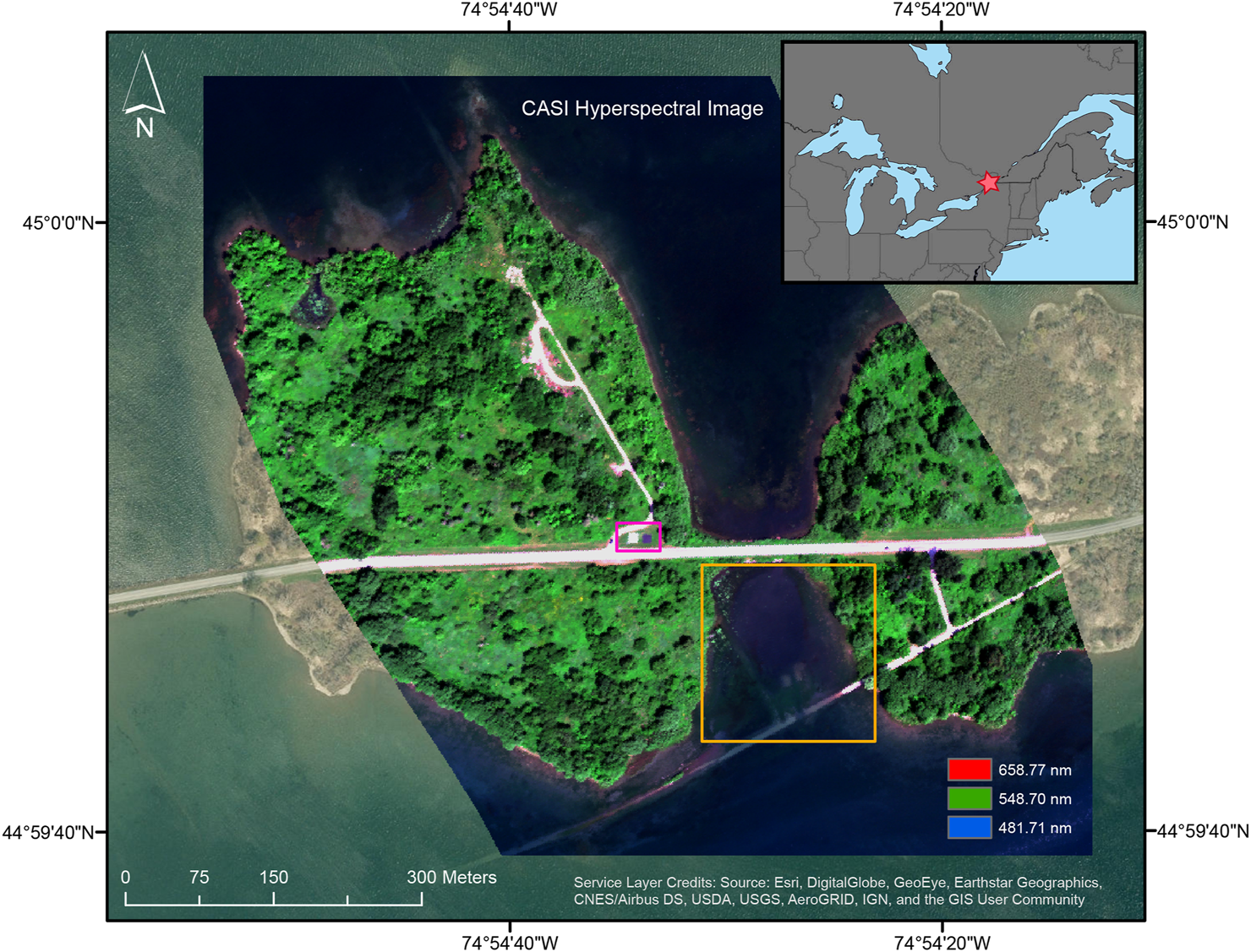
Subset of CASI airborne hyperspectral imagery (red = 658.77 nm, green = 548.70 nm, blue = 481.71 nm) presenting the study site west of Philpott’s Island in the Long Sault Parkway recreation area, Ontario, Canada. The yellow box outlines the shallow bay where samples were collected and SAV is mapped. The location of the two calibration tarps is shown in purple. The inset indicates the study site location (red star) in relation to the North American Great Lakes.
FIGURE 2
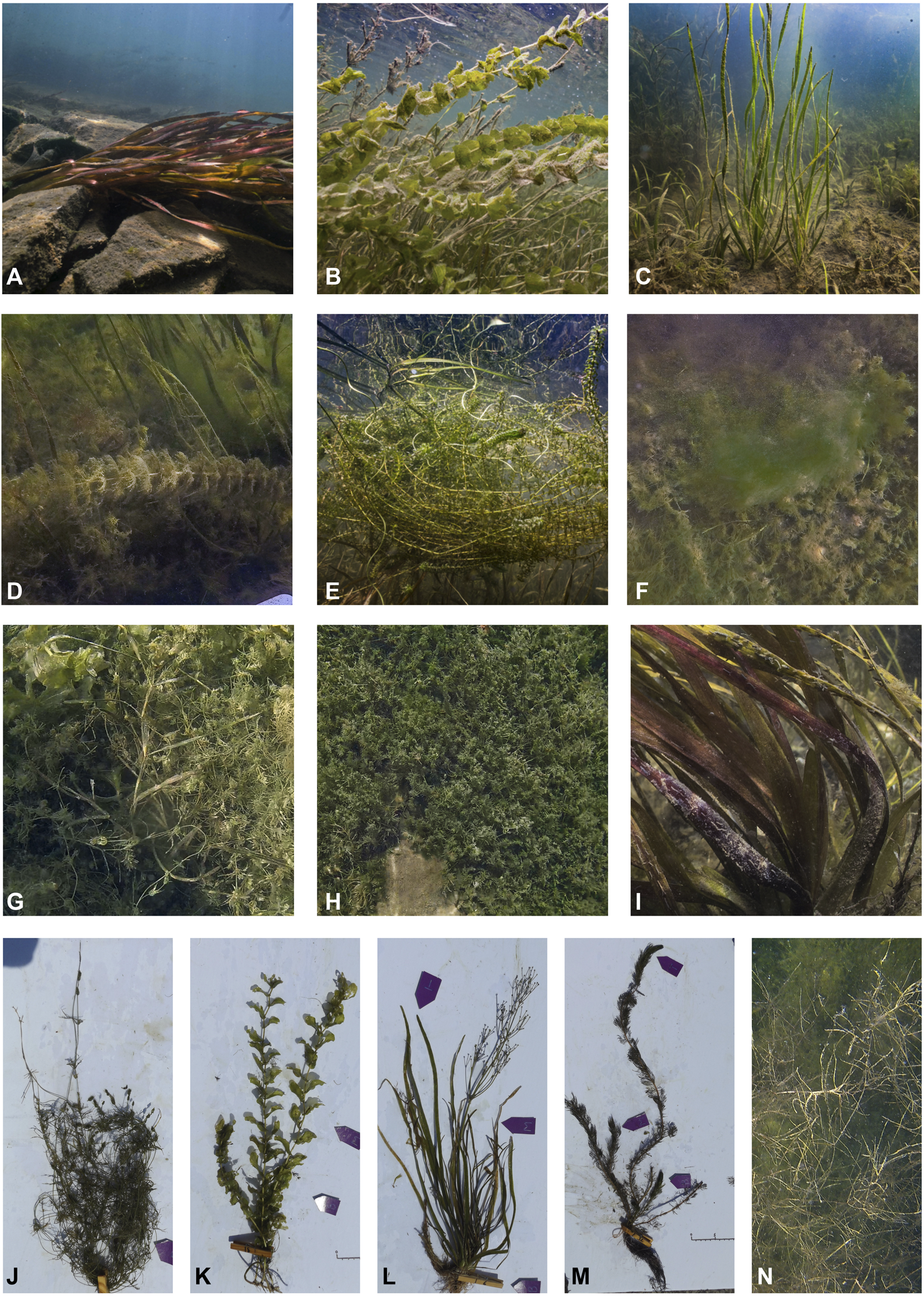
Examples of the vegetation encountered at the site (A-I) and examples of vegetation provided to expert interpreters (J-N). (A)Vallisneria americana; (B)Potamogeton richardsonii; (C)Sagittaria graminea; (D)Myriophyllum spicatum; (E)Elodea canadensis; (F) Metaphyton; (G)Potamogeton robbinsii; (H)Chara sp.; (I)Vallisneria americana with heavy leaf fouling; (J)Chara sp.; (K)Potamogeton richardsonii; (L)Sagittaria graminea; (M)Myriophyllum spicatum; (N)Potamogeton sp..
Multiscale Approach
Figure 3 shows the different levels at which SAV was assessed including leaf-level spectroscopy (i.e., finest spectral resolution), resampled air/spaceborne sensors, and actual airborne hyperspectral imagery. The following sections thoroughly describe the data acquisition, processing and analysis employed in this study. A flowchart of the analytical steps is shown in Figure 4.
FIGURE 3
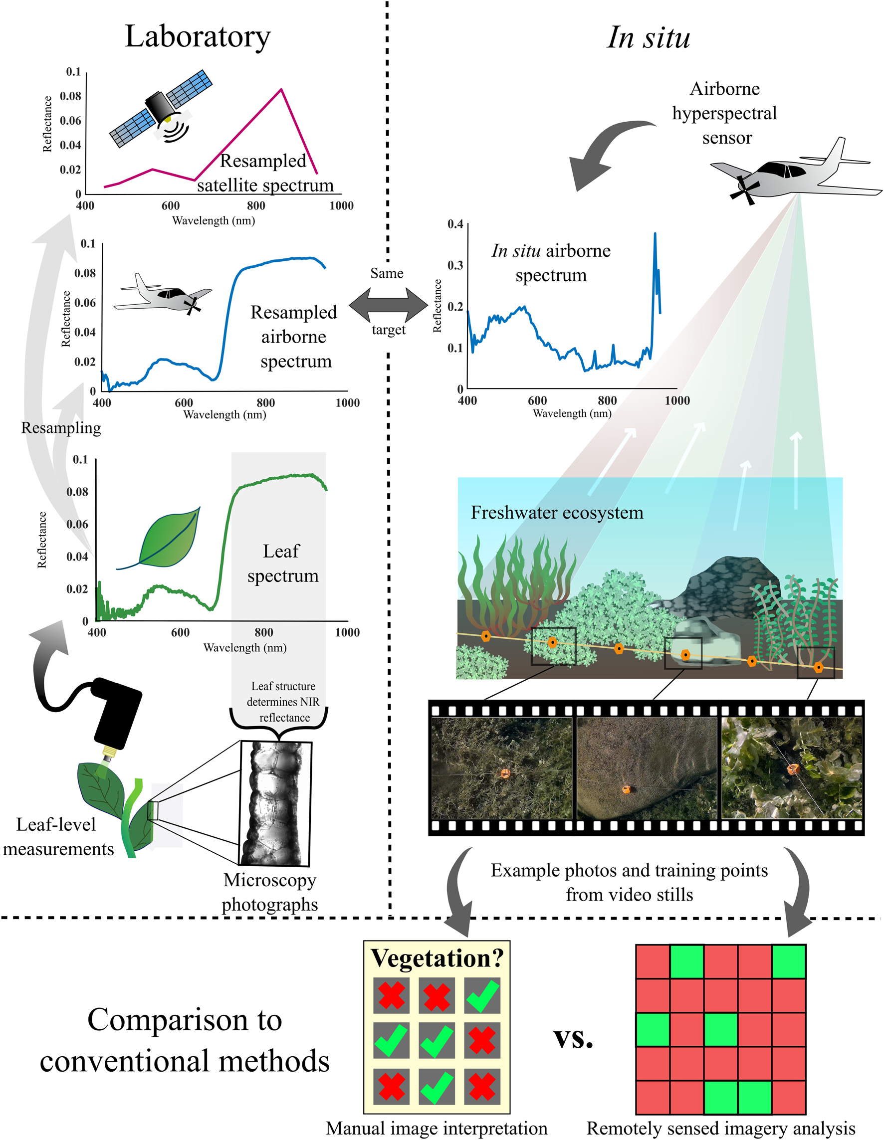
The multi-scale approach implemented in this study. Laboratory spectral measurements were collected of the leaves of each plant sample collected from the site; microscopy images of leaf cross-sections were then taken for each species to inform subsequent analysis of the leaf spectra. Leaf spectra were then resampled to an airborne and six spaceborne imaging sensors that deploy for large scale in situ applications. A shallow freshwater site was imaged using an airborne hyperspectral sensor from which spectra of the same vegetation examined in the lab could be extracted. Underwater video footage of four transects provided training and ground truth points for SAV target detection from the airborne imagery. Video stills were additionally presented to fellow researchers to be manually interpreted to present the utility of remote sensing in the context of the performance of conventional SAV monitoring methods.
FIGURE 4
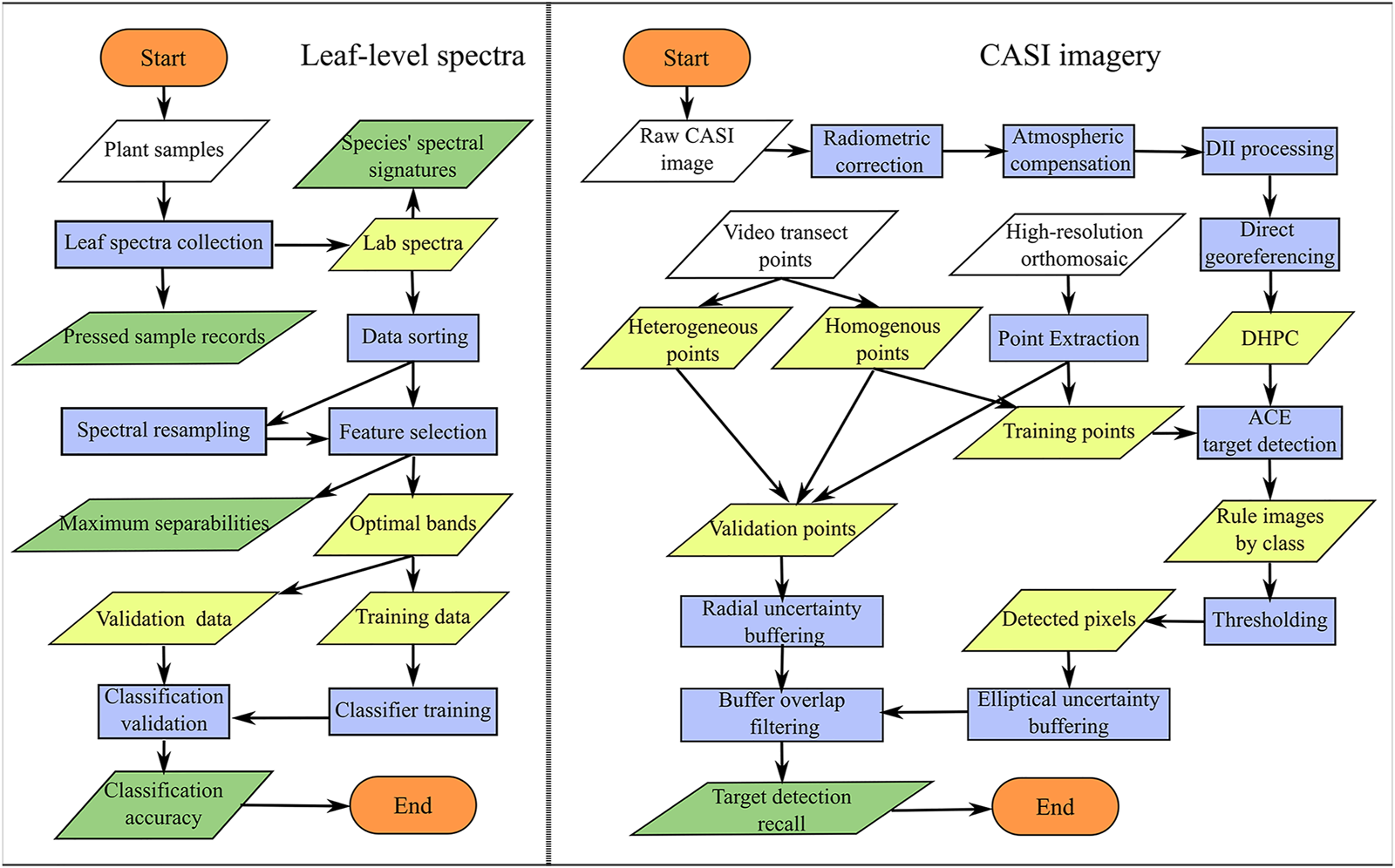
Workflow for both the leaf level spectral analysis and the processing and analysis of the CASI image.
Submerged Aquatic Vegetation Sampling
Spectralon Panel Measurements
A 99% reflective Spectralon (Labsphere, North Sutton, New Hampshire) panel was submerged to different depths to determine the absorptive properties of the water column in relation to a separate 99% reflective Spectralon panel which remained on dry land. Spectra of the panel were collected using an Analytical Spectral Devices (ASD) Fieldspec 3 spectroradiometer (Malvern Panalytical, Boulder Colorado), referred to hereafter as “ASD,” at depths from ∼1 mm to 115 cm at 5 cm intervals (Supplementary Figure S1). This instrument measures reflected radiation in the 350–2,500 nm range, has a spectral resolution of 3 nm and a sampling interval of 1.4 nm in the visible (VIS) and near infrared (NIR) regions and a spectral resolution of 10 nm with a sampling interval of 2 nm in the shortwave infrared (SWIR) (Asd Inc., 2010). Measurements were repeated at three locations within the bay for each depth and then averaged following the calculation of the estimated absolute reflectance (Rabs) according to Elmer et al. (2020) and Soffer et al. (2019).
Plant Sample Collection
Plants were collected twice: on August 5th, 2019, and on August 12th, 2020, with water temperatures of 21°C and 23.5°C, respectively. The 2020 flora was substantially more mature than the previous year, likely due to differences in springtime flooding (severe flooding in 2019 potentially delayed the growing season). Many plants were flowering in 2020 and leaves were senescing. The 2019 and 2020 samples were therefore designated as peak-growing season and late-growing season, respectively. The study area was informally surveyed by a snorkeler to identify as many species as possible and approximate their relative abundance; the plants were harvested according to those estimates. Whenever possible, plants of the same species were collected from different areas and depths to maximize intra-specific variability. Sampling in 2020 was additionally selective to find plants with healthy leaves. Two silt samples were collected in 2019. Samples were labeled, stored in river water, and transported to a dark room.
The taxonomy of each sample was determined according to Crow et al. (2000). In the cases of uncertainty at the species level, the sample was labelled to the genus level. Supplementary Table S1 presents an overview of the samples collected in both years and the coded nomenclature used throughout this work.
Microscopy
To supplement the leaf level spectral measurements (see Leaf Level Spectral Measurements) because vegetation’s NIR reflectance is strongly influenced by leaf structure (Knipling, 1970), microscopy photographs were collected of each species sampled in 2020 to qualitatively assess the structural diversity present in the SAV being studied. Images were acquired at the McGill University Multi-Scale Imaging Facility, Sainte-Anne-de-Bellevue, Québec, Canada. Plants were kept in water until being prepared for imaging, ensuring their freshness; they were neither preserved nor stained before imaging. Thin cross sections were cut across the center of each leaf, ensuring all internal structures (i.e., mesophyll, lacunae, vascular bundles, etc.) were included in the images. Cross sections were placed in a small amount of water to avoid desiccation. Photographs were taken using an AxioCam MRm Rev.2. mounted on a Zeiss AxioImager Z1 microscope equipped with an LED light and a halogen lamp for illumination. Magnifications between ×4 and ×40 were applied depending on the subject.
Ground Truth Data Collection
Ground truth points recording the locations of different SAV species in the bay were gathered to provide input and validation data for analysis of the airborne imagery. Points recording locations of exposed silt and cement and asphalt (i.e., from a submerged road and building foundations) without vegetation cover were also collected. These points were collected in two ways: recorded observations at each location of the 2019 plant sampling, and underwater video footage of four 20 m transects, each with thirty-one location markers (Supplementary Figure S1). The locations sampled and the placement of the transects were stratified to include the full variability in vegetation cover present. Sampling points were included for use in imagery analysis if they were observed to have homogeneous cover of one of the operational taxonomic units (OTUs) considered over at least ∼1 m2. Video footage of each transect was collected by tracing over the length of the transect in a square wave pattern with a Go Pro hero 5 held nadir at the surface of the water. Frames of each transect marker (124 in total) were extracted from this video and assessed to determine ground cover. Transect markers were assigned to a given OTU if the frame containing the marker was covered at least 40% by a single class; points could thus be assigned to up to two vegetation classes: unassigned points were discarded; points assigned to a single class were divided into training and validation sets; points assigned to two classes were used in validation but not training. Sampling locations and transect marker placements were recorded using a Reach RS+ (EMLID, St. Petersburg, Russia) Global Navigation Satellite System (GNSS) receiver unit according to (Kalacska, 2018), with incoming Network Transport of RTCM via Internet Protocol (NTRIP) corrections from a SmartNet North America base station located ∼25 km away in Morrisburg, Ontario.
High Spatial Resolution Orthomosaic
To supplement the input and validation data available for analysis from the ground truth points, a high spatial resolution RGB orthomosaic was produced from which additional training and validation data could be extracted. A DJI Inspire 2 Remotely Piloted Aircraft System (RPAS) with an X5S camera (micro 4/3 sensor) and a DJI MFT 15 mm/1.7 aspherical lens (72° diagonal field of view) was used to acquire photographs of the bay from an altitude of 40 m AGL. A total of 703 photographs were acquired in a double grid pattern with 85% front and side overlaps. The 20.8 MP .jpg photographs were 5,280 pixels wide by 3,956 pixels tall. Pix4D Mapper v4.7.1 was used to generate an orthomosaic following the Structure-from-Motion MultiView Stereo workflow described in (Kalacska et al., 2018). Twenty-three ground control points (GCPs) consisting of submerged targets placed throughout the bay were used to improve the positional accuracy of the orthomosaic during processing with Pix4D Mapper since the geotags of the Inspire 2 are neither real-time kinematic nor post-processing kinematic corrected (Kalacska et al., 2020). The coordinates of the GCPs were measured with the Reach RS + GNSS receiver as described above. Two hundred and forty points over areas of at least 1 m2 of homogenous ground cover were manually identified from the orthomosaic. As not all species sampled at the site grow in canopy-forming stands and some stands were homogenous by growth type rather than species, the points were limited to the following 7 classes: ribbon-like leaves (Sagittaria graminea and Vallisneria americana), Potamogeton richardsonii, metaphyton, Chara sp., Potamogeton sp., paved asphalt, and other non-vegetation (silt and rock).
Leaf-Level Spectra
Leaf-Level Spectral Measurements
The leaf-level spectra of each sample were collected in a darkroom through a modified contact measurement procedure using the ASD and a low intensity halogen contact probe. The probe ensures a constant viewing and illumination geometry with a 1 cm diameter spot. The samples were placed in a matte black dish with a ∼1–2 mm layer of water covering the leaves to avoid desiccation. The probe was placed close enough for the lens to touch the thin water layer over the leaves and a spectrum was collected over each leaf or leaf segment as there was often visible variability present within individual plants and leaves (Supplementary Table S1). The samples were measured both in their natural fouled state as well as after rinsing to remove the fouling. The 2019 samples of metaphyton, Potamogeton crispus, and Nymphaea odorata were not re-measured following rinsing due to sample degradation. The reflectance ratio of each sample acquired by the ASD was converted to Rabs following Elmer et al. (2020). Each sample was pressed in paper, dried, and kept as records locally to be deposited within a herbarium at a later date. The leaf spectra were then sorted into 7 datasets in each year according to the OTUs outlined in Supplementary Table S2.
Resampled Airborne Hyperspectral and Multi-Spectral Satellite Submerged Aquatic Vegetation Spectra
Both airborne hyperspectral and multispectral satellite imagery have a lower spectral resolution and are thus incomparable to that of the leaf level spectra collected under laboratory conditions with a spectroradiometer. It was therefore important to analyze the leaf level spectra resampled to the spectral response functions of the air/spaceborne sensors simulating how the signatures would be recorded by these coarser resolution sensors. The leaf spectra were resampled to the relative spectral response (RSR) functions of six former or current multispectral satellite sensors and an airborne hyperspectral imager, the Compact Airborne Spectrographic Imager-1500 (CASI) (Figure 5, Supplementary Table S3). See Image Acquisition and Processing for a description of the CASI. The resampled spectra then underwent the subsequent analysis described below alongside the original ASD spectra to compare results across sensors.
FIGURE 5
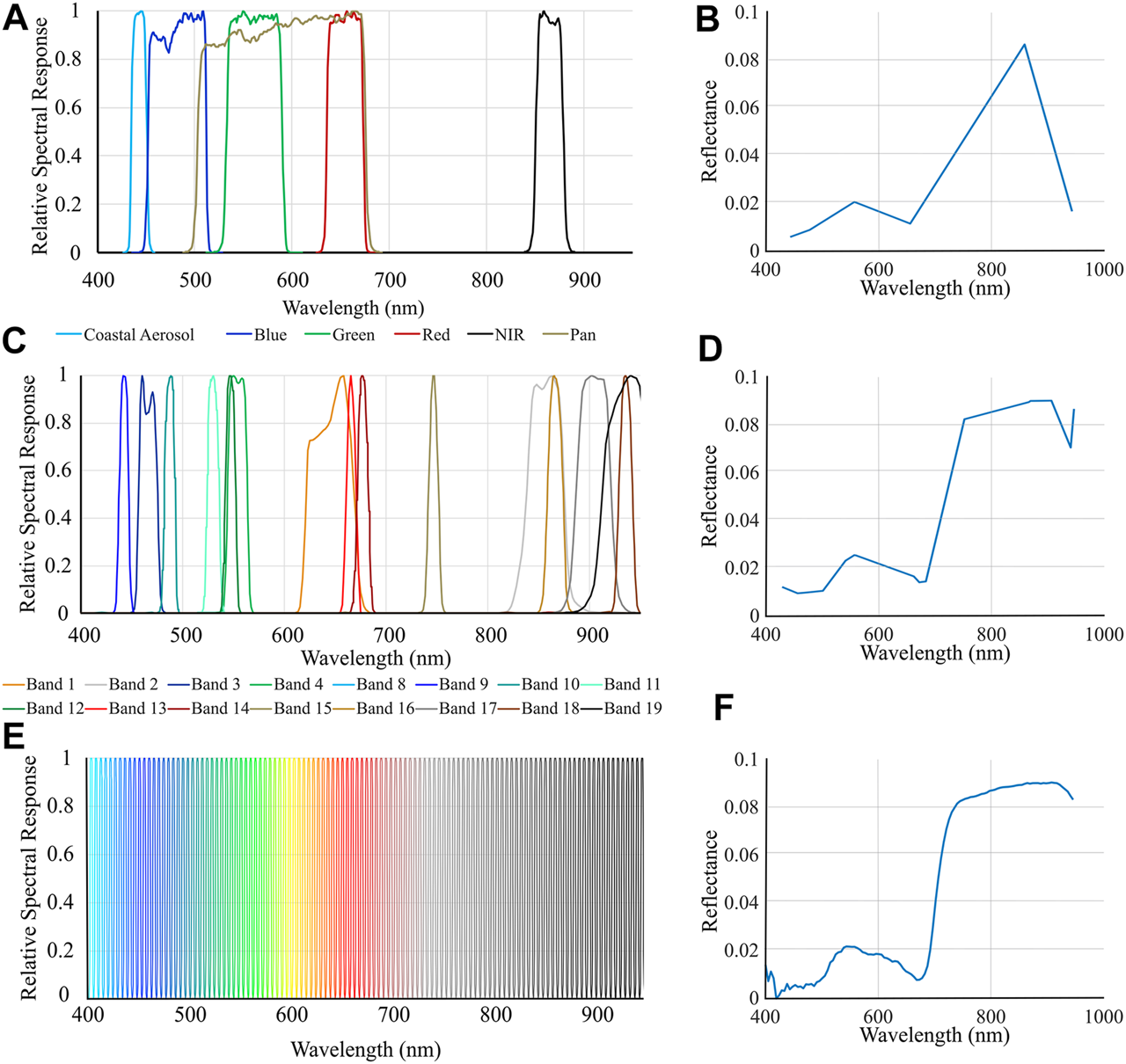
Relative Spectral Response (RSR) functions of two satellite sensors and the airborne sensor resampled to in this work for the 400–950 nm spectral range, and an example of a Vallisneria americana spectrum obtained after each spectral resampling. (A) RSR of the Landsat 8OLI sensor. (B)V. americana spectrum resampled to Landsat 8OLI. (C) MODIS’s RSR. (D)V. americana spectrum resampled to MODIS. (E) RSR of the CASI airborne hyperspectral imager. (F)V. americana spectrum resampled to the CASI.
Feature Selection and Classification
The leaf level spectra underwent dimension reduction and classification, steps that are often also applied to imagery, to determine the theoretical best separability and classification accuracy achievable for this set of SAV species. All leaf spectra were subset to the 400–950 nm range due to the artificial illumination causing substantial noise in shorter wavelengths, and the near-complete absorption of longer wavelengths by even a very thin water column, as determined from measurements of the submerged Spectralon panel (see Submerged Panel Measurements–Determination of Usable Wavelength Range). A forward feature selection (FFS) with a nearest neighbour criterion (Devijver and Kittler, 1982) was implemented in MATLAB R2020a (Mathworks, Natick Massachusetts) using the PRTools5 toolbox (Duin and Pekalska, 2016) to determine the optimal bandset to distinguish between the various OTUs. After feature selection, each dataset, reduced to the optimal bands was divided 60/40 into training and testing samples. After an initial trial run with all thirty-four classifiers in the PRTools toolbox on the peak-growing season, species level of both fouled and unfouled samples (a19 dataset; Supplementary Table S2), all classifiers that resulted in a validation accuracy ≥80% were retained and applied to all datasets (see Leaf Level and Resampled Air/Spaceborne Spectral Classification).
Airborne Hyperspectral Imagery
Image Acquisition and Processing
A 144-band airborne hyperspectral image of the study area (Figure 1) was acquired with the CASI-1500 sensor (ITRES Ltd., Calgary, AB) on July 26th, 2019, by the National Research Council of Canada’s Flight Research Laboratory (NRC-FRL) (acquisition parameters are provided in Supplementary Table S4). The image was preprocessed to units of radiance (uW/cm2/sr/nm) using lab-derived calibration parameters applied using standard processing modules as provided by the manufacturer (Soffer et al., 2019). Because surface water results in a weak signal, conventional radiometric correction procedures developed for imagery of terrestrial environments result in radiance values that are erroneously low and often negative at wavelengths below 450 nm (Soffer et al., 2021). As such, a two-part, non-linear In-Flight Radiometric Refinement (IFRR) methodology following Soffer et al. (2021) specifically developed for pixel spectral responses equivalent to surface reflectance levels <3% was applied prior to atmospheric correction.
The IFRR refined radiance image was then atmospherically corrected with ATCOR4 v7.3.0. to generate surface reflectance (Figure 4; Supplementary Table S4). To compensate for the effect of the water column, the Depth Invariant Index (DII) (Lyzenga, 1978; Lyzenga, 1981) was calculated for all band pairs including only wavelengths below 950 nm (Inamdar et al., 2021c, submitted). A maximum correlation coefficient threshold of 0.9 was applied to reduce the dimensionality of the DII data from 5,565 (all pairs) to 124. Following the methodology described in (Inamdar et al., 2021a; Inamdar et al., 2021b), the DII bands were geocorrected without raster resampling to generate a hyperspectral point cloud which assigns 3D spatial coordinates to each image spectrum without introducing the pixel duplications and loss that result from conventional nearest neighbour raster resampling. Next, in CloudCompare v2.12, the point cloud was subset to the study site and was rasterized to 25 cm pixels (empty cells were not interpolated over) to allow data visualization of the point cloud in raster data format without introducing pixel loss or duplication; NoData values were given to empty cells. In ENVI v5.5.3 (Harris Geospatial Solutions, Inc., Broomfield, CO), all NoData pixels were masked out. Ground truth points (Submerged Aquatic Vegetation Ground Truth Data Collection) and points extracted from the orthomosaic (High Spatial Resolution Orthomosaic) were imported into ENVI and the nearest DII data pixel to each was manually selected and assigned the point’s label, sometimes resulting in a single data pixel being assigned multiple ground truth point labels.
Target Detection
Target detection was used to identify SAV classes in the airborne HSI as not all materials in the HSI were known and the classes covered relatively small areas. A target detection was performed in ENVI on the 124 band DII image for each of the classes of interest (i.e., five canopy-forming vegetation types, the paved asphalt road, silt/rock, all vegetation combined, and a non-vegetation class). The selected pixels corresponding to the ground truth and orthomosaic points were divided 60/40 into input (target and non-target) spectra and validation points. The Adaptive Coherence Estimator (ACE) algorithm (Scharf and McWhorter, 1996) (Eq. (1)) was used to create rule images for each class with all other classes input as non-target spectra. Assignment thresholds were then selected to maximize the detection of known class extent while minimizing false positive detections (Supplementary Table S5). ACE was chosen for its ability to detect sub-pixel targets as was common at the field site due to the small areal extent of most SAV stands and is calculated as follows:where ST is the mean input spectrum of the target class after undergoing a matrix transposition, x is the pixel spectrum under consideration and b is the covariance matrix of the classes identified as non-target background (Manolakis and Shaw, 2002).
Accuracy Assessment
To account for the spatial uncertainty in both the reported locations of the ground truth data and the geocorrection of the CASI imagery, buffers were created around all detected pixels and validation points according to the spatial uncertainty of each data set. For the validation points recorded in situ, the buffer diameter was calculated as the sum of the manufacturer reported accuracy for NTRIP baselines >10 km (i.e., 1 m) and the average standard deviation of the points reported by the Reach RS + unit (Elmer and Kalacska, 2021). For the pixels output from the target detection, the uncertainty buffer considered the reported spatial accuracy of the CASI imagery (2.25 m) (Elmer and Kalacska, 2021) and the effective pixel resolution, the area corresponding to the full-width half -max of the CASI’s point spread function (Inamdar et al., 2021a) (i.e., 1.038 m in the across-track and 0.978 m in the along-track) as determined following (Inamdar et al., 2021b). The sum of the spatial accuracy and the effective pixel resolution resulted in elliptical uncertainty boundaries where materials contributing to each pixel’s recorded signal were located. Validation points were deemed to have been correctly detected if the point’s and the pixel’s buffers overlapped.
Expert Visual Interpretation
To assess the relative utility of employing remote sensing methods to aquatic vegetation monitoring, the validation accuracy of the target detections performed on the imagery was compared to the accuracy a team of researchers could achieve by manually inspecting the same vegetation OTUs. Field assistants that had participated in this fieldwork, and select external researchers with experience in botany and/or remote sensing, interpreted 135 pictures from the field site consisting of field photos and frames extracted from the underwater video transects. All pictures were color corrected to improve their interpretability. The pictures were made available online similar to the implementation described by Danylo et al. (2021). The online platform chosen to host the pictures and record the selections was SurveyLegend (surveylegend.com). The content consisted of three sections: first, examples of vegetation were presented; second, expert interpreters identified photos with at least 40% of the frame covered by a specified vegetation type; and third, expert interpreters selected all photos with any amount of a specified vegetation type. It is acknowledged that this method did not account for user expertise or the choice of photos included; it is presented strictly as a coarse estimate of manual detection accuracy.
Results
Submerged Panel Measurements–Determination of Usable Wavelength Range
The average Rabs measurements of the Spectralon panel submerged across depths up to 115 cm are shown in Figure 6. In general, as expected, the reflected signal decreases in amplitude with increasing depth (Figure 6A). The reflectance of the panel in the VIS wavelengths (450–650 nm) does not however demonstrate consistent exponential decay across all depths; at certain wavelengths (e.g., 440 nm), increased reflectance values at lower depths were recorded (Figure 6B). Beyond 900 nm, there is strong absorption by the water column with reflectance <0.06 for any depth of 5 cm or more. For all depths of more than 15 cm, reflectance is <0.02 at wavelengths greater than 950 nm, indicating that spectral information from almost all aquatic targets would be limited to wavelengths shorter than 950 nm.
FIGURE 6
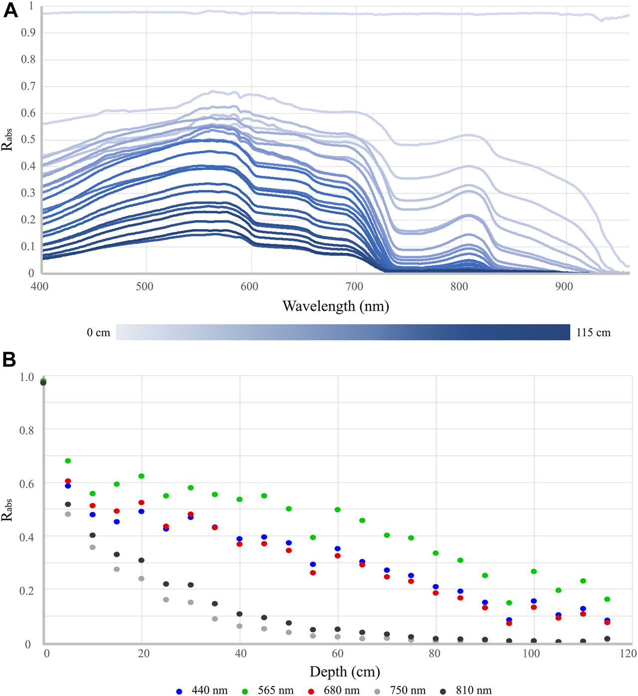
Effect of the water column on the reflectance of a submerged 99% Spectralon panel. (A) Estimated Absolute Reflectance (Rabs) at 5 cm depth intervals between ∼0 and 115 cm. (B) Rabs at select VIS (440 nm, 565 nm, and 680 nm) and NIR (750 and 810 nm) wavelengths plotted against panel submergence depth.
Leaf Spectroscopy
Impact of Biofouling and Season
The average laboratory spectra for each leaf-level OTU for each year (Supplementary Table S2) are shown in Figure 7. While all plant and algae spectra have the expected spectral signature of green vegetation (Gates et al., 1965) the amplitude is low, especially in the NIR (<0.27). Fouling had only a minimal effect on the spectra (Supplementary Figure S2A,B, Supplementary Figure S3A). Averaged across all species, removing the fouling produced a maximum difference in the reflectance amplitude of 3.9% at 921 nm in the peak-growing season and of 1.1% at 900 nm in the late-growing season, with the average difference ranging from −0.1 to 3.9% and from −1.1 to 0.5%, respectively. Seasonality had a more varied effect on mean spectra across species (Supplementary Figure S2C,D, Supplementary Figure S3C,D). The maximum difference in reflectance between peak-growing season and late-growing season samples, averaged across all species, was 4.5% at 921 nm in fouled samples and 1.3% at 909 nm in unfouled samples, with the average differences between seasons ranging from -1.6 to 4.5% and -1–1.3%, respectively.
FIGURE 7
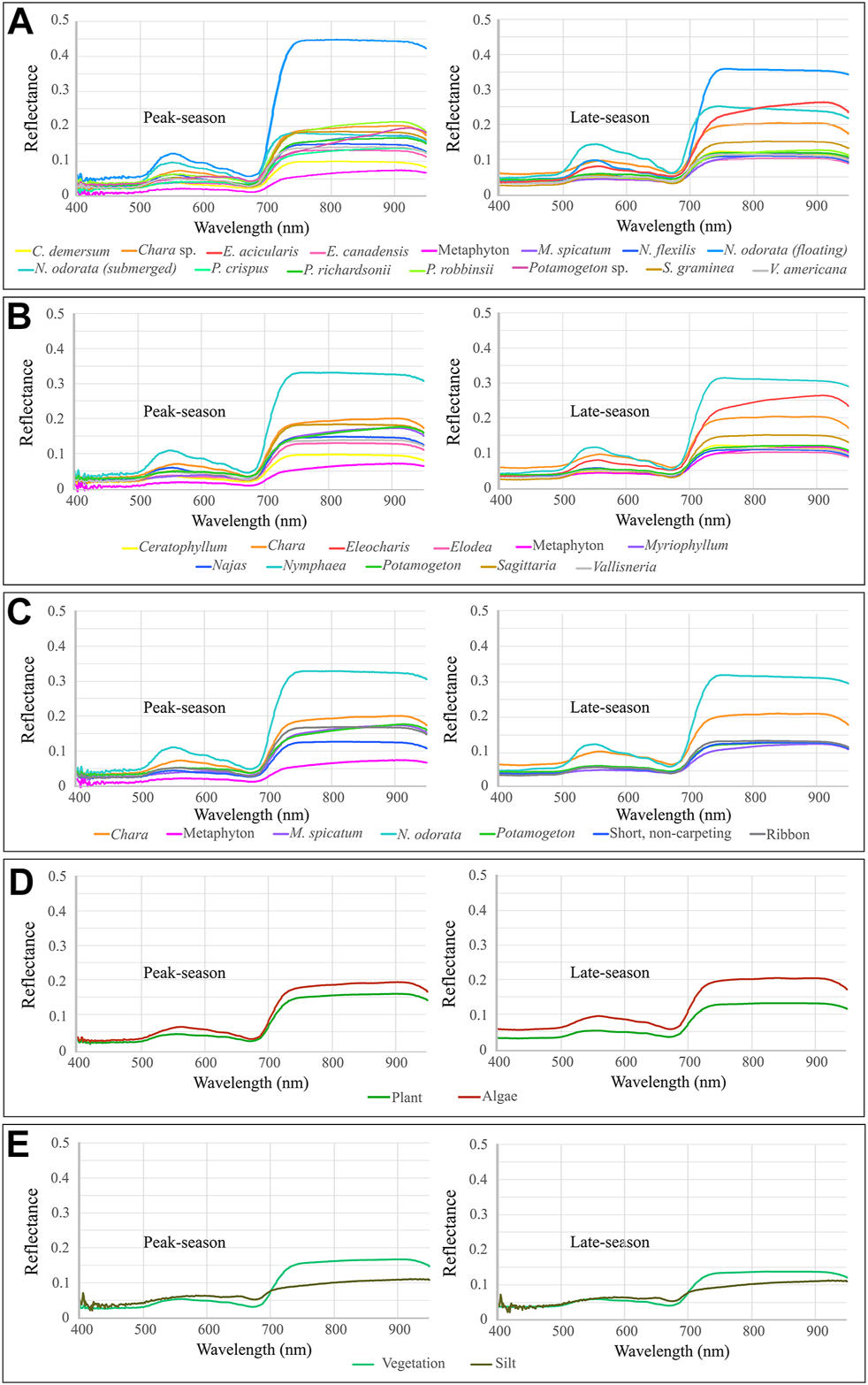
Average spectra of all classes in each grouping scheme for both 2019 and 2020. (A) All samples grouped by species (a19 and a20); (B) All samples grouped by genus (p19 and p20); (C) All samples in ad hoc grouping (g19 and g20); (D) All samples grouped by kingdom (alga19 and alga20); (E) All vegetation samples plus silt samples grouped as vegetation or non-vegetation (s19 and s20).
Forward Feature Selection Across Operational Taxonomic Units
The forward feature selection produced ranked lists of features (i.e., bands) according to the marginal contributions of each wavelength to maximum theoretical separability (Leave-one-out Nearest Neighbor criterion (LNN)) for each dataset for each sensor (Supplemental Figures S4 and S5, Tables 1, 2). In both seasons and across all OTUs, features in the VIS tended to be higher ranked than those in the NIR (Supplemental Figure S4). In the peak-growing season samples, five of the seven OTUs most important contributors to separability were near the Chl-a reflectance peak (∼550 nm), with the other two top ranked features located in the total pigment absorbance peak (∼450 nm) and the red edge region (∼700 nm). In the late-growing season however, five out of seven OTUs top-ranked feature were located in the NIR region; the majority of subsequent highly ranked wavelengths remained in the VIS. In every case, most of the maximum separability between classes can be attributed to just a few of the top ranked wavelengths (Supplemental Figures S5). Ninety five percent of the total separability between classes could be achieved with at most 24 of the top ranked bands (out of a maximum 551 bands). Increasing the separability from 95% to the maximum value could require >200 additional input bands (Table 1).
TABLE 1
| Dataset grouping, fouling, season (code) | Max LNN | 95% of max LNN | No. features selected to max LNN | No. features to 95% of max LNN |
|---|---|---|---|---|
| By species, fouled, peak-growing season (f19) | 0.84 | 0.80 | 38 | 10 |
| By species, unfouled, peak-growing season (u19) | 0.82 | 0.77 | 281 | 13 |
| By species, combined, peak-growing season (a19) | 0.80 | 0.76 | 276 | 23 |
| By genus, combined, peak-growing season (p19) | 0.81 | 0.77 | 258 | 14 |
| Ad hoc, combined, peak-growing season (g19) | 0.84 | 0.80 | 267 | 10 |
| By kingdom, combined, peak-growing season (alga19) | 0.98 | 0.93 | 52 | 4 |
| Vegetation/non-vegetation, combined, peak-growing season (s19) | 1.00 | 0.95 | 58 | 1 |
| By species, fouled, late-growing season (f20) | 0.56 | 0.53 | 32 | 19 |
| By species, unfouled, late-growing season (u20) | 0.55 | 0.52 | 57 | 15 |
| By species, combined, late-growing season (a20) | 0.55 | 0.52 | 238 | 15 |
| By genus, combined, late-growing season (p20) | 0.56 | 0.54 | 162 | 15 |
| Ad hoc, combined, late-growing season (g20) | 0.62 | 0.59 | 64 | 10 |
| By kingdom, combined, late-growing season (alga20) | 0.98 | 0.93 | 13 | 3 |
| Vegetation/non-vegetation, combined, late- growing season (s20) | 1.00 | 0.95 | 6 | 1 |
Results of the forward feature selection algorithm for the full resolution ASD spectra. The 95% of maximum LNN criterion value and number of features required to produce 95% of the maximum separability are included as many selected features provide only marginal gains in separability.
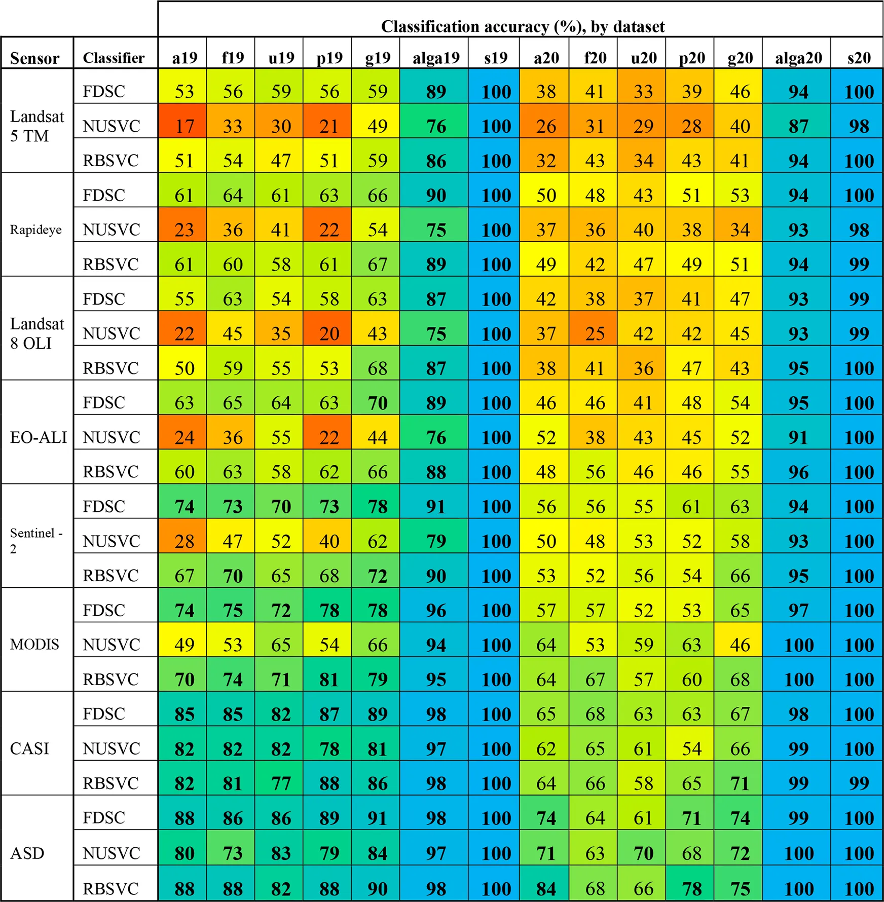
TABLE 2
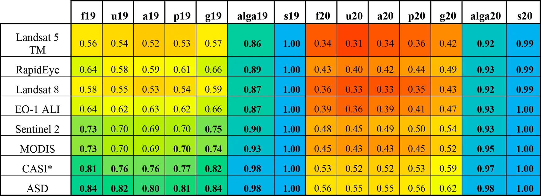 |
Maximum LNN values for each grouping and year for the original (ASD) spectra and all resampled spectra. Multi and hyperspectral sensors to which the spectra were resampled are ordered by increasing spectral information (No. bands). Cells have been coloured according to their value for rapid interpretation (gradient: red = 0.2, yellow = 0.6, blue = 1). All values above 0.7 have been bolded for easy identification. *CASI is an airborne hyperspectral imager, all others are multi-spectral spaceborne sensors.
The original laboratory spectra produced the highest separability values in all cases (Table 2). On a scale from 0 (classes entirely inseparable) to 1 (classes perfectly separable), the peak-growing season samples had LNN criterion values ranging from 0.8 (all samples, grouped by species) to 1 (vegetation/non-vegetation) depending on the coarseness of the OTU definition. The late-growing season samples had LNN criterion values between 0.55 (unfouled and all samples, grouped by species) and 1 (vegetation/non-vegetation). While separation between kingdoms and between vegetation/non-vegetation were equally high (0.98 and 1, respectively) in both years, the more granular OTUs were found to be sensitive to the effect of seasonality; peak-growing season samples were more separable than late-growing season samples (e.g., LNN values 0.80 and 0.55 for the species level OTU from the peak-growing season and late-growing season samples, respectively). A slight improvement in separability (from 0.82 to 0.84 and from 0.55 to 0.56 for peak-growing season and late-growing season samples, respectively) was seen in the fouled samples as compared to the unfouled samples, in both years (Table 2).
Leaf Cross Sections
Cross-section photographs of the leaves taken via microscope revealed common patterns in leaf structure, largely divided between the plants with thin flat leaves (E. canadensis, P. richardsonii, P. robbinsii, S. graminea, V. americana) and those with compound leaflets (C. demersum, N. flexilis, M. spicatum) or exclusively stems (E. acicularis) (Supplementary Figure S6). In all plants, large lacunae were visible (or developing) with a single layer of large mesophyll cells dividing them. There were no disaggregated intra-cellular air spaces as is common in the spongy mesophyll of terrestrial, emergent, and floating vegetation (Supplementary Figure S6G), nor was there columnar mesophyll in any submerged leaves. Thin flat leaves tended to only be a few cells thick except for in proximity to a vascular bundle where the cells were smaller and more densely packed. Leaflets and stems were roughly circular with up to four large central lacunae and radial thicknesses of only a few cells. Chara sp., a macroalgae, was distinct from the plants in lacking all interior structure.
Resampled Airborne Hyperspectral Imagery and Multispectral Satellite Spectral Separability
Resampling the spectra to the RSRs of space- and air-borne sensors (Figure 5) clearly demonstrates the dependence of separability on spectral resolution and number of bands (Table 2). For example, spectra resampled to the RSR of Landsat TM5 resulted in LNN separability on the fouled, peak-growing season species level OTU of 0.56, compared to 0.84 from the original ASD spectra. This pattern of increasing separability with increasing spectral resolution and number of bands was consistent across resampled datasets (Table 2). The theoretical LNN separability from all RSR resampled spectra was found to be adequately (>0.70) high to separate spectra between kingdoms and between vegetation/non-vegetation OTUs in both years. Spectra resampled to the RSRs of Sentinel-2, MODIS and the CASI (airborne hyperspectral) produced acceptably high separability values for the species level OTUs from the peak-growing season fouled and unfouled samples (i.e., 0.73 and 0.70, 0.73 and 0.70, and 0.81 and 0.76, respectively), as well as for the genus level OTU from the peak-growing season samples (0.70, 0.70, and 0.77, respectively) and the ad hoc OTU (0.75, 0.74, and 0.82, respectively) (Table 2).
Leaf-Level and Resampled Air/Spaceborne Spectral Classification
Classification accuracy (at the species level OTU from the peak-growing season with both fouled and unfouled spectra) with the FDSC, NUSVC, and RBSVC classifiers was >80% (Supplementary Table S1). Classification accuracies across OTUs for each of those three classifiers are presented in Table 3. Although the NUSVC performed well on the leaf level spectroradiometer data, it resulted in 26 and 23% lower accuracy at the species level than FDSC and RBSVC, respectively. The accuracies of the FDSC and RBSVC classifiers were similar across OTUs, years, and resampled sensors, with the resultant classification accuracies being similar to the maximum theoretical separability determined for each dataset (Table 3).
TABLE 3
 |
Classification accuracy of the FSDC, NUSVC, and RBSVC classifiers for each grouping and year for the original (ASD) and all resampled spectra. Accuracy values have been colour coded for rapid interpretation (gradient: red = 0, yellow = 0.5, blue = 1). All values above 0.7 have been bolded for easy identification. Datasets are described in Supplementary Table S3.2.
Imagery
High-Spatial Resolution RGB Orthomosaic
The Structure from Motion photogrammetry (703 UAS photographs) produced a high-spatial resolution orthomosaic with a ground sampling distance of 1.16 cm (Figure 8A). Pix4D Mapper found a median of 71,013 key points per photograph (435 photographs out of the 703 input were calibrated), and a median of 1,489.9 matches between adjacent photographs. The mean residual root mean square error in the positional accuracy of the orthomosaic related to the GCPs was 1.14 m. The blank spaces in the lower middle section of the final orthomosaic are due to the interference of surface glare which precluded identifying key points in those areas (Figure 8A).
FIGURE 8

CASI imagery used in this work at various processing stages and the input points used in target detection and validation. (A) RPAS orthomosaic showing points of each class chosen through visual interpretation and the locations of the transect points. (B) Atmospherically compensated CASI image (red = 687.5 nm, green = 548.7, blue = 500.3 nm, optimized linear stretch applied on extent) before geocorrection. (C) DII-transformed CASI image following rasterization of the directly georeferenced point cloud without resampling (red = 682.7 and 701.8 nm DII, green = 553.5 and 563.1 nm DII, blue = 424.3 and 438.7 nm DII, linear stretch on extent applied). Each pixel is a 25 cm by 25 cm visualization of the set of DIIs centered at the coordinates calculated to be where the signal originated from. (D) Conventionally geocorrected CASI imagery after atmospheric compensation, for reference.
Airborne Hyperspectral Imagery Target Detection
The atmospherically corrected CASI HSI image and the directly-georeferenced DII image are presented in Figures 8B,C. SAV was detected in 5,444 pixels (5,527 m2, 0.55 ha) of the total 65,160 water pixels (66,148 m2, 6.6 ha) contained in the DII image. Likewise, non-vegetation substrate was detected in 2,518 pixels (2,556 m2, 0.26 ha) (Supplementary Table S2). A total of 6,368 pixels (6,465 m2, 0.65 ha) were detected to contain one of the seven more granular target classes. The range of the ACE detection statistic attributable to mixed pixels varied widely across classes, though the mean ACE value of the mixed pixels was never greater than the threshold value (Figure 9). For some classes, such as metaphyton and non-vegetation, the range of the ACE detection statistic values representing mixed pixels is exceedingly small, perhaps indicating that the points considered mixed pixels did not contain enough of the material to produce an identifiable spectral contribution.
FIGURE 9
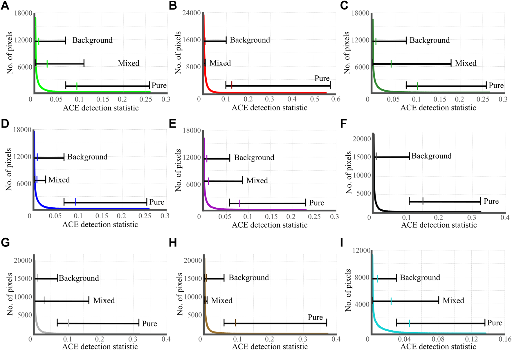
Results of the ACE target detection. Curves depict the number of pixels according to the ACE detection statistic assigned. Horizontal bars indicate the range of ACE detection statistic values attributable to each type of pixel (pure target, mixed target, background) with the mean value indicated by a coloured tick mark. Pure and background pixels are separated at the threshold values presented in Table SM3.6; mixed pixel ranges were determined according to ACE detection statistic values of mixed transect points. (A)Chara sp. (B) Metaphyton. (C)P. richardsonii. (D)Potamogeton sp. (E) Ribbon. (F) Road, no mixed pixels identified. (G) Silt/Rock. (H) Non-vegetation. (I) Vegetation.
Target Detection Validation
An example of the target detection validation for Potamogeton sp. is shown in Figure 10. In this example, pure points of Potamogeton cover were detected in 10 of 13 instances, resulting in a recall of 77%; mixed pixels were however poorly detected with only one of nine mixed pixels detected (combined pure and mixed pixel recall of 50%). Overall, the target detections, for the OTUs and the binary vegetation/non-vegetation classes, were effective, especially when considering validation points representing pure pixels (Table 4). The target detection validation with pure pixels resulted in an overall, average accuracy of 87.8% across the individual OTUs and two non-vegetation classes, and 93.6% for the binary vegetation/non-vegetation classes. Including mixed pixels (i.e., points with more than one cover type present) in the validation reduced the overall accuracy of the target detection to an average of 67.0% across the OTUs. In this case the label of each class with >40% areal coverage was assessed. The asphalt class was perfectly recalled, and the silt/rock class achieved 94% recall, however 408 (414 m2, 0.04 ha) instances of asphalt were detected in the silt/rock class. The metaphyton class was poorly recalled; potentially due to the limited training and validation data or due to biophysical properties of the metaphyton itself. The binary vegetation and non-vegetation classes were very well detected (recall of 94%). Notably, 5 of the 6 instances of missed vegetation (false negatives) represented points of ribbon-like plants (V. americana and S. graminea).
FIGURE 10

Example of validation for the Potamogeton sp. target detection with grey ellipses around detected pixels, pure validation points, mixed validation points, and validation points correctly detected identified. Conventionally geocorrected true colour CASI image shown in background for context. Insets are underwater photograph examples of pure Potamogeton sp. (A) and mixed (B)Potamogeton sp. and Chara sp. cover. In this example, 10 of the 13 pure cover points were detected shown by the green circles; one mixed cover point was detected.
TABLE 4
| Class | Pure pixels only | Pure and mixed pixels | ||||
|---|---|---|---|---|---|---|
| No. Validation points | True Positives | Recall (%) | No. Validation points | True Positives | Recall (%) | |
| Chara sp | 24 | 19 | 79 | 81 | 53 | 65 |
| Metaphyton | 2 | 0 | 0 | 4 | 0 | 0 |
| P. richardsonii | 6 | 6 | 100 | 20 | 18 | 90 |
| Ribbon | 18 | 15 | 83 | 32 | 20 | 63 |
| Potamogeton sp | 13 | 10 | 77 | 22 | 11 | 50 |
| Road | 20 | 20 | 100 | 20 | 20 | 100 |
| Silt/Rock | 17 | 16 | 94 | 51 | 32 | 63 |
| Overall | 98 | 86 | 88 | 230 | 154 | 67 |
| Vegetation | 56 | 50 | 89 | — | — | — |
| Non-vegetation | 38 | 38 | 100 | — | — | — |
| Overall | 94 | 88 | 94 | — | — | — |
Validation results of the target detection analyses. Mixed pixels are identified as having at least 40% cover of the class in question.
Expert Interpretation
Twelve visual interpreters each completed the manual online SAV identification. The true positives from the visual interpreters are shown in Figure 11, alongside true positives of the ACE target detection validation. Generally, the visual interpreters accurately identified extensive (>40% areal coverage) SAV cover, with class recall rates of between 67 and 96%. Detection of individual plants was however less effective and consistent, with recall between 49 and 89% (Figure 11). While manual image interpretation was more successful at detecting most of the SAV OTUs, higher recall values were achieved using ACE for detecting Chara sp. and P. richardsonii at the species level. There was a wide variability in interpretation responses, for example in the detection of extensive P. richardsonii or ribbon-like plants as seen in Figure 11, suggesting that in situ manual observations of vegetation by those who are not already closely acquainted with the plants may not be accurate.
FIGURE 11
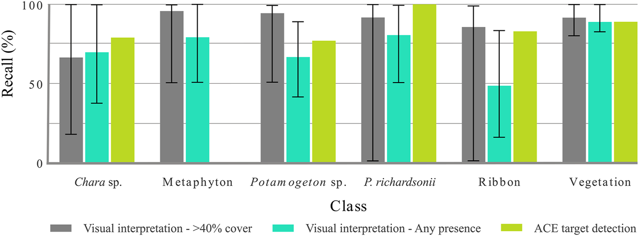
Comparison of recall results from visual interpretation, for both 40% class cover and any instance of class presence, and CASI airborne hyperspectral image target detection. The range of responses is shown by the error bars for visual interpretation results.
Discussion
The leaf level separability analysis has shown that freshwater SAV does indeed contain sufficient spectral diversity within the VIS and NIR to be reliably separated with hyperspectral data across various OTU definitions (Table 2). In situ mapping of that same set of SAV, while successful overall, highlights that the use of remote sensing in monitoring SAV is limited by the spatial resolution of imagery available.
Water Column Impacts
Our submerged panels measurements reveal that the usable spectral region was limited to wavelengths <950 nm due to the strong absorption of radiation by water in the NIR (Figure 6). Although 950 nm is somewhat more restrictive than the maximum wavelength used in other work (e.g., 1,050 nm by Visser et al. (2013) and 1,000 nm by Brooks et al. (2019)), the selection of this upper limit is supported by water’s third harmonic absorption peak at ∼960 nm, after which absorption remains high (Kirk, 1994). Therefore, future work should expect useful information exclusively from the VIS (e.g., up to 700 nm) and shortest wavelengths in the NIR regardless of bathymetry for all water types. As little as 5 cm of submergence reduced the panel Rabs to 0.66 at 550 nm and to 0.34 at 900 nm. Under a 40 cm thick water column, Rabs reduced further to 0.52 at 550 nm and 0.00 at 900 nm (Figure 6). A very high signal-to-noise ratio (SNR) would hence be necessary to meaningfully capture radiance from underwater targets (e.g., Muller-Karger et al. (2018) cite an SNR of 800 as sufficient for aquatic studies). However, even upcoming sensors conceptualized specifically for aquatic applications are not expected to meet such high SNR demands (e.g., PRISM has a SNR of 500 in the blue region (Mouroulis et al., 2014); PACE is expected to have an SNR ranging from 400 to 1700 (Werdell et al., 2019)).
Leaf Spectroscopy
Effect of Biofouling and Season
At the leaf level, confirming previous findings by Fyfe. (2003), it was found that light fouling had very little effect on species mean reflectance signatures though it did mask some intra-class variability in the NIR (Supplementary Figure S1A,B), which may explain the minor, yet positive, effect fouling produced on class separability in both years (Table 2). As neither the fouling load nor its composition were examined, the relationship between fouling and spectral response cannot be here defined. Still, these results are encouraging for future mapping efforts in fluvial freshwaters such as the St. Lawrence River where light fouling is common. As expected, season substantially affected the SAV species spectral signatures (Supplementary Figure S2B). Increased variability was prominent in the late-growing season samples compared to their peak-growing season counterparts (Supplementary Figure S2C,D) potentially due to the increased relative concentration of accessory pigments later in the growing season (Salisbury and Ross, 1992; Gitelson and Merzlyak, 1994). This evolution in leaf spectral response through senescence, combined with the recorded changes in spectral response as a young leaf matures (Gates et al., 1965), indicate that SAV spectral measurements are temporally distinct and could be used to estimate plant maturity.
Leaf-Level Feature Selection and Separability
Physiological changes occurring within leaves throughout maturation were reflected in the features selected as important contributors to class separability (Figure 8). Mesophyll thickness, intra-cellular space, and leaf thickness determine the number of multiple refractions within a leaf and mediate NIR reflectance, previously shown in terrestrial plants (Castro-Esau et al., 2006). The lack of structural complexity and diversity in the SAV leaves examined here (Supplementary Figure S6) thus explain the NIR’s irrelevance in achieving spectral separability in the peak-growing season. However, the introduced structural diversity in the late-growing season due to uneven senescence resulted in NIR features to contribute most to separability for the majority of the OTUs (e.g., 938 and 809 nm were top ranked for discriminating across all species and between vegetation and non-vegetation, respectively).
Besides changes in leaf and cellular structure, the selected features mirrored the evolution of pigment concentrations throughout the growing season. The Chl-a reflectance peak, referred to as the green peak (∼550 nm) was the primary contributor to spectral separability for most OTUs during the peak-growing season when plants invest in Chl-a production. Chl-a absorptance was comparatively unimportant later in the summer when Chl-a is less abundant due to increased shading (Maksimović et al., 2020) and plants redirect resources toward accessory pigments (Salisbury and Ross, 1992). This temporal variability in relative pigment abundance also explains the substantial increase in moderately to highly ranked features in the red and red edge regions (650–710 nm). The total pigment absorptance feature (∼445 nm) was the most important contributor to separability in both years when distinguishing between plants and algae possibly due to the differences in pigment composition and content between the two kingdoms (UC Museum of Paleontology, 2001). The dissimilarity in selected features between the two seasons signifies that the spectral response of SAV is temporally specific; data collected in the peak of summer should not be used to train or validate work done on later in the summer, or vice versa.
Contradictory to previous work (Klemas, 2013), the decrease in OTU class separability in the late-growing season suggests that SAV monitoring campaigns should target the peak-growing season to maximize accuracy. The maximum separability between classes (Table 2) is also related directly to the coarseness of the OTUs. Though aggregating multiple similar species into more coarsely defined classes such as genera (rather than species) increases the intra-class spectral variability, it can likewise increase inter-class variability, improving classification results. Although this study is the first instance of it being documented in vascular aquatic plants, the improvement in class separability in higher-level OTUs has previously been demonstrated in macroalgae (species vs clade) and trees (population vs species) (Cavender-Bares et al., 2016; McIlwaine et al., 2019). Interestingly, class separability increased not only across progressively higher taxa but also in the combination of species into the ad hoc group that was not exclusively based on evolutionary proximity. While spectral similarity may relate to a common phenotype or functional group, shared traits cannot be assumed to confer the spectral similarity that would produce accurate classification (Laliberté et al., 2020). The high separability of the ad hoc group (Table 2) is therefore encouraging for ecosystem managers that may be interested in classes other than taxonomy, like growth type.
Resampled Air and Spaceborne Sensor Spectra
Even though high spectral separability was obtained after resampling the leaf level spectra to the RSRs of Sentinel-2 and MODIS (Table 2), these resampled spectra model a signal originating from a single species (i.e., pure pixels) and do not account for the uncertainties of even the most accurate radiometric, atmospheric and water column corrections, conditions that cannot be met with actual imagery. To be reliably detected in imagery, targets need to be at least twice the length of a pixel’s diagonal (Heblinski et al., 2011). Patches of vegetation would thus need to be at least 28 m in diameter to be detected by Sentinel-2’s 10 m pixels; only one stand of vegetation of this size was observed in this study, while all others were much smaller (<10 m in diameter). Reliable detection in MODIS pixels would require patches over 282 m in diameter. The spatial resolution of current spaceborne sensors thus precludes their use with many in-land freshwater ecosystems in which such large extents of vegetation are rare. Past sensors, such as Landsat TM5 and EO-1 ALI, had been included to examine the feasibility of retrospective analysis on archived data (Table 2). While the retrieval of historical images to extend time series is common in other fields, the poor separability between all but the coarsest OTUs (i.e., the binary vegetation/non-vegetation classes) severely restricts the utility of archived satellite imagery in SAV research.
In contrast to the satellites, very good separability (LNN criterion values of between 0.76 and 1 for the species-level OTU of unfouled samples and the vegetation/non-vegetation OUT, respectively) was achieved for peak-growing season spectra resampled to the CASI RSR for all OTUs (Table 2). This is unsurprising, given the CASI’s high spectral resolution in terms of both band width and number of bands. As the CASI is an airborne sensor, the high spatial resolution (∼1 m pixel size) is also much better suited to the spatial distribution patterns of SAV than spaceborne platforms. Airborne hyperspectral imagery such as that produced by the CASI is thus expected to be appropriate for SAV mapping.
Imagery
Airborne Hyperspectral Imagery Depth Invariant Index
A novel DII transformation (Inamdar et al., 2021c; Lyzenga 1978, Lyzenga, 1981) based on a hyperspectral point cloud as opposed to conventional geocorrected, resampled raster imagery (Inamdar et al., 2021a; Inamdar et al., 2021b) was implemented to optimize the data quality of the CASI imagery. While Lyzenga’s DII may be highly effective at distinguishing between bottom cover types, its performance depends entirely on the two input bands. If two (or more) targets do not reflect differently in the two wavelengths chosen, a DII calculated using those bands will not be unique to either material (Lyzenga, 1978). Considering that two materials may be spectrally alike in some, but not all pairs of wavelengths, computing all possible DIIs ensures that the spectral diversity in the signals is represented. A set of all possible DII values however increases the data dimensionality, rendering it (in the case of hyperspectral data) computationally unfeasible (i.e., 5565 DII bands from a 106 input-band image). The DII transformation used here addressed this by sub-setting all possible DIIs to only those below a 0.9 covariance threshold. Thus, most unique spectral information was retained, the imagery dimension was limited, and the water column was compensated for. Work by Mumby et al. (1998) demonstrated that implementing as few as two DII bands and some contextual editing could improve bottom cover classification accuracy (between 4 and 13 classes) by up to 23%. It is thus expected that maximizing the number of DII bands with unique information would similarly increase mapping accuracy. However, if reliable bathymetric information is available, empirical methods such as that described in Purkis and Pasterkamp. (2004) could be used to retrieve relative bottom reflectance as opposed to the transformed DII values, facilitating interpretation. By rasterizing the georeferenced DII point cloud without resampling (Figure 9), the original image acquisition geometry was respected and facilitated extraction of the target DII spectra and validation points based on the RGB orthomosaic and field sampling. Furthermore, because the goal of this study was fine scale target detection, it was critical to preserve all pixels captured in the raw imagery. The Directly-georeferenced Hyperspectral Point Cloud method implemented here was shown to substantially reduce target detection false negatives due to pixel loss over conventionally georeferenced and resampled raster imagery (Inamdar et al., 2021a); applying this method therefore maximized the number of potential target pixels included in the analysis.
Airborne Hyperspectral Imagery Target Detection
The ACE detection statistic thresholds were chosen to discern known areas of class cover and minimize false positives. These thresholds were strict, as shown in Figure 9 by the mean mixed pixel always being outside the target class range. It is thus unlikely that these sub-pixel targets could be effectively detected without producing many false positives. The target classes were limited to the OTUs present in patches of similar size to the CASI pixel resolution (∼1 m) to avoid classes of uniquely sub-pixel targets. Hence, not all SAV species included in the leaf level analysis were targets in the imagery (e.g., E. canadensis and M. spicatum were both abundant at the site, but did not form large, monotypic stands). If a sparse or non-canopy forming species, such as the invasive M. spicatum were of critical interest, monitoring efforts would require imagery on the scale of a few centimeters such as that produced from RPAS-mounted sensors (e.g., Arroyo-Mora et al., 2019).
The ACE target detections identified points of pure bottom cover well, particularly for the binary vegetation/non-vegetation classes (Table 4; Figure 10). ACE uses target and non-target input spectra to estimate and disregard noise that is shared between the two groups. It produces a single statistic value that is invariant to changes in scaling (such as might be produced by changes in signal strength due to variable water column thickness) (Kraut et al., 2005). Previous work by Flynn and Chapra. (2014) confirms the utility of ACE in mapping aquatic targets by correctly detecting Cladophora extent with 90% accuracy. Macfarlane et al. (2021) additionally determined the ACE algorithm to be most effective in airborne hyperspectral target detection in a cross-comparison of five target detection processes. As ACE uses all input target spectra to calculate a mean target profile, it is unsurprising that five of the six false negative vegetation points were in dense patches of ribbon-like plants. These plants (S. graminea and V. americana) tended to be visibly darker and redder than other species (Figure 2) and were, in some areas, sufficiently dark to be confused with deep water pixels. Thus, spectra of these dense stands were too different from the average of all vegetation (mostly greener and brighter) (Figure 7) to be detected without introducing innumerable false positives. Separating the darker, redder vegetation into its own class may thereby be more effective. The very good overall detection recall across vegetation types (Table 4) suggests that a similar methodology would be of use in management situations in which the growth type is of interest, such as in maintaining clear navigation corridors or preventing the establishment of tall vegetation near water intakes.
Manual Field Photograph Interpretation
Manual interpretation of field photographs was conducted to compare the performance of traditional surveys of SAV and the remote sensing methodology used here. Interpreters completed two tasks (selecting images that presented >40% cover of a specified bottom type and identifying all images with any instance of the specified bottom type) to simulate detection of full-pixel and sub-pixel targets. Recall values were not substantially different between manual detection of extensive bottom cover and the ACE target detection of pure pixels (Figure 11), suggesting that the remote sensing methods used here could produce similarly accurate results to in person surveys conducted by researchers that are not already well acquainted with the vegetation. Photograph interpretation for sub-pixel target identification was generally less successful, with more response variability. This decrease in manual interpretation success mirrors the decline in recall of the ACE target detections when including mixed pixels in the validation set (Table 4). While manual interpretation remains more effective at detecting targets over a small area, the remote sensing methods used here provided acceptable target detection rates and could be applied to a larger spatial scale by a smaller team.
Overall Importance
Our results show that the SAV examined do present enough spectral diversity to be separable despite the limited spectral range available in aquatic remote sensing and the general lack of identifying information in the NIR. That separability extends beyond taxonomic groupings, having been observed in the ad hoc grouping roughly based on phenotype. Mapping and identifying SAV through optical remote sensing are therefore anticipated to be an appropriate tool in a broad range of management and research applications. Using airborne hyperspectral imagery to map that same SAV demonstrated that very high detection rates can be achieved for targets of a similar size to the imagery pixels. The increasing availability of RPAS platforms, and thereby higher spatial resolution imagery, is expected to further extend the scope of aquatic targets suited to detection and mapping through remote sensing. This work has shown that optical remote sensing is indeed a viable alternative to manual surveys for monitoring SAV in shallow clear to moderate optical water types from freshwater ecosystems, and its spectrum of potential uses is still growing.
Conclusion
To address some of the fundamental knowledge gaps remaining in the application of optical remote sensing to freshwater ecosystems identified by Rowan and Kalacska. (2021), the spectral separability amongst thirteen SAV species was examined under laboratory conditions and through actual airborne imagery. Implementing a multi-scale approach provided insight into what is currently possible for researchers/practitioners working across scales and with varying resources and highlighted future possibilities from further technological innovation and investment. The species of SAV were reliably separable under laboratory conditions from leaf-level spectroradiometer data, with light leaf fouling having minimal effect but seasonality being an important determinant of separability. As the samples were found to be less separable late in the growing season than at its peak, it is recommended that future studies consider avoiding late-growing season data collection. Additionally, separability was improved with progressively higher-level OTUs (i.e., genus or kingdom). Resampling the leaf level spectra to simulate spaceborne sensors reduced separability, demonstrating that most publicly available satellite data products do not have the necessary spectral resolution required for reliable SAV separation; those that do, lack the high spatial resolution needed to study freshwater SAV communities. Resampling the leaf level spectra to simulate the CASI, an airborne hyperspectral sensor, produced high separability results. Combining this high separability with the fine spatial resolution achievable from airborne platforms, airborne HSI with similar spatial and spectral characteristics could be amenable to SAV monitoring applications. Detecting instances of target vegetation and bottom cover from the airborne HSI was effective, though it was limited to cover types occurring in patches of similar size to the imagery pixels, meaning not all species at the site could be detected. Before SAV can be operationally mapped in freshwaters across broad spatial extents, higher resolution spaceborne sensors and more precise pre-processing workflows for low signal level targets are needed. The enhanced radiometric correction (i.e., IFRR) used here enhanced the useable low-level signals and the novel DII transformation allowed for an effective water column compensation. Importantly, the directly-georeferenced point cloud data model ensured maximal retention of information and spatial integrity. These improvements over conventional aquatic remote sensing workflows are thus recommended for application in future SAV monitoring and mapping endeavors. Freshwater SAV has here been shown to contain sufficient spectral diversity for reliable separation, though the success of in situ applications remains limited by the spectral and spatial resolution of available data.
Statements
Data availability statement
The datasets presented in this article are available from the corresponding author upon request following the CABO data use agreement from https://cabo.geog.mcgill.ca. Requests to access the datasets should be directed to margaret.kalacska@mcgill.ca.
Author contributions
Conceptualization, GSLR and MK; formal analysis, GSLR; funding and resource acquisition, JPA-M, RS, and MK; methodology, GSLR and MK; software, DI; visualization, GSLR and JPA-M; writing—original draft preparation, GSLR; writing—review and editing, all authors listed have made a substantial, direct, and intellectual contribution to the work and approved it for publication.
Funding
This research was supported by the Natural Sciences and Engineering Research Council (NSERC), the Canadian Airborne Biodiversity Observatory (CABO), and a Rathlyn Fellowship in GIS (Rowan). Airborne hyperspectral image acquisition was funded by the National Research Council of Canada.
Acknowledgments
We would like to thank Oliver Lucanus for his help in collecting underwater and RPAS imagery of the site, as well as Erica-Skye Schaaf, Kathryn Elmer, Patrick Osei-Darko, Elias Vitali, George Rowan, and Laura Logan for their assistance in the field and laboratory data collection. Thanks to Dr. H. Peter White and Prof. Andrew Hendry for their constructive comments. Additional thanks are given to Dr. Youssef Chebli for his assistance in collecting the microscopy photographs, and to Brent Sommerville and Liam Carson from the St Lawrence Parks Commission for facilitating access to the study site.
Conflict of interest
The authors declare that the research was conducted in the absence of any commercial or financial relationships that could be construed as a potential conflict of interest.
Publisher’s note
All claims expressed in this article are solely those of the authors and do not necessarily represent those of their affiliated organizations, or those of the publisher, the editors and the reviewers. Any product that may be evaluated in this article, or claim that may be made by its manufacturer, is not guaranteed or endorsed by the publisher.
Supplementary material
The Supplementary Material for this article can be found online at: https://www.frontiersin.org/articles/10.3389/fenvs.2021.760372/full#supplementary-material
References
1
Arroyo-MoraJ.KalacskaM.InamdarD.SofferR.LucanusO.GormanJ.et al (2019). Implementation of a UAV-Hyperspectral Pushbroom Imager for Ecological Monitoring. Drones3 (1), 12. 10.3390/drones3010012
2
Arroyo-MoraJ. P.KalacskaM.LøkeT.SchläpferD.CoopsN. C.LucanusO.et al (2021). Assessing the Impact of Illumination on UAV Pushbroom Hyperspectral Imagery Collected under Various Cloud Cover Conditions. Remote Sensing Environ.258, 112396. 10.1016/j.rse.2021.112396
3
Asd Inc (2010). FieldSpec 3 User Manual.
4
AsnerG. P.KnappD.BalajiA.Paez-AcostaG. (2009). Automated Mapping of Tropical Deforestation and forest Degradation: CLASlite. J. Appl. Remote Sens3 (1), 033543. 10.1117/1.3223675
5
BrooksC. N.GrimmA. G.MarcarelliA. M.DobsonR. J. (2019). Multiscale Collection and Analysis of Submerged Aquatic Vegetation Spectral Profiles for Eurasian Watermilfoil Detection. J. Appl. Rem. Sens.13 (3), 1. 10.1117/1.Jrs.13.037501
6
Castro-EsauK. L.Sánchez-AzofeifaG. A.RivardB.WrightS. J.QuesadaM. (2006). Variability in Leaf Optical Properties of Mesoamerican Trees and the Potential for Species Classification. Am. J. Bot.93 (4), 517–530. 10.3732/ajb.93.4.517
7
Cavender-BaresJ.MeirelesJ.CoutureJ.KaprothM.KingdonC.SinghA.et al (2016). Associations of Leaf Spectra with Genetic and Phylogenetic Variation in Oaks: Prospects for Remote Detection of Biodiversity. Remote Sensing8(3),221. 10.3390/rs8030221
8
ChenQ.YuR.HaoY.WuL.ZhangW.ZhangQ.et al (2018). A New Method for Mapping Aquatic Vegetation Especially Underwater Vegetation in Lake Ulansuhai Using GF-1 Satellite Data. Remote Sensing10 (8), 1279. 10.3390/rs10081279
9
ClarkM.RobertsD.ClarkD. (2005). Hyperspectral Discrimination of Tropical Rain forest Tree Species at Leaf to crown Scales. Remote Sensing Environ.96 (3-4), 375–398. 10.1016/j.rse.2005.03.009
10
CochraneM. A. (2000). Using Vegetation Reflectance Variability for Species Level Classification of Hyperspectral Data. Int. J. Remote Sensing21 (10), 2075–2087. 10.1080/01431160050021303
11
CrowG. E.HellquistC. B.FassettN. C. (2000). Aquatic and Wetland Plants of Northeastern North America: A Revised and Enlarged Edition of Norman C. Fassett's a Manual of Aquatic Plants. Madison: University of Wisconsin Press.
12
DanyloO.PirkerJ.LemoineG.CeccheriniG.SeeL.McCallumI.et al (2021). A Map of the Extent and Year of Detection of Oil palm Plantations in Indonesia, Malaysia and Thailand. Sci. Data8 (1), 96. 10.1038/s41597-021-00867-1
13
DevijverP. A.KittlerJ. (1982). Pattern Recognition: A Statistical Approach. Englewood Cliffs, N.J.: Prentice/Hall International.
14
DierssenH. M.AcklesonS. G.JoyceK. E.HestirE. L.CastagnaA.LavenderS.et al (2021). Living up to the Hype of Hyperspectral Aquatic Remote Sensing: Science, Resources and Outlook. Front. Environ. Sci.9 (134). 10.3389/fenvs.2021.649528
15
DuffyJ. E.Benedetti-CecchiL.TrinanesJ.Muller-KargerF. E.Ambo-RappeR.BoströmC.et al (2019). Toward a Coordinated Global Observing System for Seagrasses and Marine Macroalgae. Front. Mar. Sci.6. 10.3389/fmars.2019.00317
16
DuinR. P. W.PekalskaE. (2016). Pattern Recognition: Introduction and Terminology, 77, Delft University of Technology.
17
ElmerK.KalacskaM. (2021). A High-Accuracy GNSS Dataset of Ground Truth Points Collected within Îles-De-Boucherville National Park, Quebec, Canada. Data6 (3), 32. 10.3390/data6030032
18
ElmerK.SofferR. J.Arroyo-MoraJ. P.KalacskaM. (2020). ASDToolkit: A Novel MATLAB Processing Toolbox for ASD Field Spectroscopy Data. Data5 (4), 96. 10.3390/data5040096
19
FlynnK.ChapraS. (2014). Remote Sensing of Submerged Aquatic Vegetation in a Shallow Non-turbid River Using an Unmanned Aerial Vehicle. Remote Sensing6 (12), 12815–12836. 10.3390/rs61212815
20
FyfeS. K. (2003). Spatial and Temporal Variation in Spectral Reflectance: Are Seagrass Species Spectrally Distinct. Limnol. Oceanogr.48 (1 II), 464–479. 10.4319/lo.2003.48.1_part_2.0464
21
GatesD. M.KeeganH. J.SchleterJ. C.WeidnerV. R. (1965). Spectral Properties of Plants. Appl. Opt.4 (1), 11–20. 10.1364/ao.4.000011
22
GiardinoC.BrescianiM.ValentiniE.GasperiniL.BolpagniR.BrandoV. E. (2015). Airborne Hyperspectral Data to Assess Suspended Particulate Matter and Aquatic Vegetation in a Shallow and Turbid lake. Remote Sensing Environ.157, 48–57. 10.1016/j.rse.2014.04.034
23
GitelsonA.MerzlyakM. N. (1994). Spectral Reflectance Changes Associated with Autumn Senescence of Aesculus Hippocastanum L. And Acer Platanoides L. Leaves. Spectral Features and Relation to Chlorophyll Estimation. J. Plant Physiol.143 (3), 286–292. 10.1016/S0176-1617(11)81633-0
24
HarperM.MejbelH. S.LongertD.AbellR.BeardT. D.BennettJ. R.et al (2021). Twenty-five Essential Research Questions to Inform the protection and Restoration of Freshwater Biodiversity. Aquat. Conservation: Mar. Freshw. Ecosyst.10.1002/aqc.3634
25
HeblinskiJ.SchmiederK.HeegeT.AgyemangT. K.SayadyanH.VardanyanL. (2011). High-resolution Satellite Remote Sensing of Littoral Vegetation of Lake Sevan (Armenia) as a Basis for Monitoring and Assessment. Hydrobiologia661 (1), 97–111. 10.1007/s10750-010-0466-6
26
HestirE. L.SchoellhamerD. H.GreenbergJ.Morgan-KingT.UstinS. L. (2016). The Effect of Submerged Aquatic Vegetation Expansion on a Declining Turbidity Trend in the Sacramento-San Joaquin River Delta. Estuaries and Coasts39 (4), 1100–1112. 10.1007/s12237-015-0055-z
27
InamdarD.KalacskaM.Arroyo-MoraJ. P.LeblancG. (2021a). The Directly-Georeferenced Hyperspectral Point Cloud: Preserving the Integrity of Hyperspectral Imaging Data. Front. Remote Sens.2 (9). 10.3389/frsen.2021.675323
28
InamdarD.KalacskaM.LeblancG.Arroyo-MoraJ. P. (2021b). Implementation of the Directly-Georeferenced Hyperspectral point Cloud. MethodsX8, 101429. 10.1016/j.mex.2021.101429
29
InamdarD.KalacskaM.LeBlancG.Arroyo-MoraJ. P. (2021c). Characterizing and 940 Mitigating Sensor Generated Spatial Correlations in Airborne Hyperspectral Imaging 941 Data. Remote Sens.12, 641. 10.3390/rs12040641
30
International Joint Commission (2003). St. Lawrence River: Area of Concern Status Assessment. Available: https://ijc.org/sites/default/files/C185.pdf (Accessed June 28, 2021).
31
JohansenK.DuanQ.TuY.-H.SearleC.WuD.PhinnS.et al (2020). Mapping the Condition of Macadamia Tree Crops Using Multi-Spectral UAV and WorldView-3 Imagery. ISPRS J. Photogrammetry Remote Sensing165, 28–40. 10.1016/j.isprsjprs.2020.04.017
32
KalacskaM. (2018). Emlid GPS NTRIP Protocol V1. Protocols.io. 10.17504/protocols.io.qs8dwhw
33
KalacskaM.LucanusO.Arroyo-MoraJ.LalibertéÉ.ElmerK.LeblancG.et al (2020). Accuracy of 3D Landscape Reconstruction without Ground Control Points Using Different UAS Platforms. Drones4 (2), 13. 10.3390/drones4020013
34
KalacskaM.LucanusO.SousaL.VieiraT.Arroyo-MoraJ. (2018). Freshwater Fish Habitat Complexity Mapping Using above and Underwater Structure-From-Motion Photogrammetry. Remote Sensing10 (12), 1912. 10.3390/rs10121912
35
KirkJ. T. O. (1994). Light and Photosynthesis in Aquatic Ecosystems. Cambridge, Great Britain: Cambridge University Press.
36
KlemasV. (2013). Remote Sensing of Emergent and Submerged Wetlands: An Overview. Int. J. Remote Sensing34 (18), 6286–6320. 10.1080/01431161.2013.800656
37
KniplingE. B. (1970). Physical and Physiological Basis for the Reflectance of Visible and Near-Infrared Radiation from Vegetation. Remote Sensing Environ.1 (3), 155–159. 10.1016/S0034-4257(70)80021-9
38
KrautS.ScharfL. L.ButlerR. W. (2005). The Adaptive Coherence Estimator: a Uniformly Most-Powerful-Invariant Adaptive Detection Statistic. IEEE Trans. Signal. Process.53 (2), 427–438. 10.1109/tsp.2004.840823
39
LalibertéE.SchweigerA. K.LegendreP. (2020). Partitioning Plant Spectral Diversity into Alpha and Beta Components. Ecol. Lett.23 (2), 370–380. 10.1111/ele.13429
40
Lawrence SeawaySt. (2021). Let the Flooding Begin. Directed by Rasky, H. Canada.
41
LillesandT. M.KieferR. W.ChipmanJ. W. (2008). Remote Sensing and Image Interpretation. Hoboken, NJ: John Wiley & Sons.
42
LyzengaD. R. (1978). Passive Remote Sensing Techniques for Mapping Water Depth and Bottom Features. Appl. Opt.17 (3), 379–383. 10.1364/AO.17.000379
43
LyzengaD. R. (1981). Remote Sensing of Bottom Reflectance and Water Attenuation Parameters in Shallow Water Using Aircraft and Landsat Data. Int. J. Remote Sensing2 (1), 71–82. 10.1080/01431168108948342
44
MaasriA.JähnigS. C.AdamescuM. C.AdrianR.BaigunC.BairdD.et al (2021). A Global Agenda for Advancing Freshwater Biodiversity Research. EcoEvoRxiv [Preprint]. 10.32942/osf.io/4pg7f
45
MacfarlaneF.MurrayP.MarshallS.WhiteH. (2021). Investigating the Effects of a Combined Spatial and Spectral Dimensionality Reduction Approach for Aerial Hyperspectral Target Detection Applications. Remote Sensing13 (9), 1647. 10.3390/rs13091647
46
MaksimovićT.LolićS.KukavicaB. (2020). Seasonal Changes in the Content of Photosynthetic Pigments of Dominant Macrophytes in the Bardača Fishpond Area. Ekológia (Bratislava)39(3),201–213. 10.2478/eko-2020-0015
47
ManolakisD.ShawG. (2002). Detection Algorithms for Hyperspectral Imaging Applications. IEEE Signal. Process. Mag.19 (1), 29–43. 10.1109/79.974724
48
MartinM. E.NewmanS. D.AberJ. D.CongaltonR. G. (1998). Determining forest Species Composition Using High Spectral Resolution Remote Sensing Data. Remote Sensing Environ.65 (3), 249–254. 10.1016/S0034-4257(98)00035-2
49
MassicotteP.BertoloA.BrodeurP.HudonC.MingelbierM.MagnanP. (2015). Influence of the Aquatic Vegetation Landscape on Larval Fish Abundance. J. Great Lakes Res.41 (3), 873–880. 10.1016/j.jglr.2015.05.010
50
McIlwaineB.Rivas CasadoM.LeinsterP. (2019). Using 1st Derivative Reflectance Signatures within a Remote Sensing Framework to Identify Macroalgae in Marine Environments. Remote Sensing11 (6), 704. 10.3390/rs11060704
51
Ministere de l’Environment et de la Lutte Contre les Changements Climatiques (2005). Entente sur les Ressources en Eaux Durables du Bassin des Grands Lacs et du Fleuve Saint-Laurent. Available: https://www.environnement.gouv.qc.ca/eau/grandslacs/2005/ (Accessed July 1, 2021).
52
MouroulisP.Van GorpB.GreenR. O.DierssenH.WilsonD. W.EastwoodM.et al (2014). Portable Remote Imaging Spectrometer Coastal Ocean Sensor: Design, Characteristics, and First Flight Results. Appl. Opt.53 (7), 1363–1380. 10.1364/AO.53.001363
53
Muller-KargerF. E.HestirE.AdeC.TurpieK.RobertsD. A.SiegelD.et al (2018). Satellite Sensor Requirements for Monitoring Essential Biodiversity Variables of Coastal Ecosystems. Ecol. Appl.28 (3), 749–760. 10.1002/eap.1682
54
MumbyP. J.ClarkC. D.GreenE. P.EdwardsA. J. (1998). Benefits of Water Column Correction and Contextual Editing for Mapping Coral Reefs. Int. J. Remote Sensing19 (1), 203–210. 10.1080/014311698216521
55
PagnuccoK. S.MaynardG. A.FeraS. A.YanN. D.NalepaT. F.RicciardiA. (2015). The Future of Species Invasions in the Great Lakes-St. Lawrence River basin. J. Great Lakes Res.41, 96–107. 10.1016/j.jglr.2014.11.004
56
PurkisS. J.PasterkampR. (2004). Integrating In Situ Reef-Top Reflectance Spectra with Landsat TM Imagery to Aid Shallow-Tropical Benthic Habitat Mapping. Coral Reefs23 (1), 5–20. 10.1007/s00338-003-0351-0
57
Raisin Region Conservation Authority (2021). Wildlife and Habitat Restoration. Available: https://www.rrca.on.ca/page.php?id=21 (Accessed June 28, 2021).
58
RaskyH. (1954). St. Lawrence Seaway: Let the flooding begin [Television]. In CBC Newsmagazine. Canada: Canadian Broadcasting Corporation. Available at: https://www.cbc.ca/archives/entry/st-lawrence-seaway-let-the-flooding-begin.
59
RowanG. S. L.KalacskaM. (2021). A Review of Remote Sensing of Submerged Aquatic Vegetation for Non-specialists. Remote Sensing13 (4), 623. 10.3390/rs13040623
60
SalisburyF. B.RossC. W. (1992). Plant Physiology. Belmont, California: Wadworth Publishing Company.
61
SandersJ. T.JonesE. A. L.MinterA.AustinR.RobersonG. T.RichardsonR. J.et al (2021). Remote Sensing for Italian Ryegrass [Lolium Perenne L. Ssp. Multiflorum (Lam.) Husnot] Detection in Winter Wheat (Triticum aestivum L.). Front. Agron.3 (50). 10.3389/fagro.2021.687112
62
SantosM. J.KhannaS.HestirE. L.GreenbergJ. A.UstinS. L. (2016). Measuring Landscape-Scale Spread and Persistence of an Invaded Submerged Plant Community from Airborne Remote Sensing. Ecol. Appl.26 (6), 1733–1744. 10.1890/15-0615
63
ScharfL. L.McWhorterL. T. (1996). “Adaptive Matched Subspace Detectors and Adaptive Coherence Estimators”, in: Conference Record of The Thirtieth Asilomar Conference on Signals, Systems and Computers), Pacific Grove, CA, USA, 3-6 Nov. 1996, IEEE, 1114–1117 vol. 1112. 10.1109/ACSSC.1996.599116
64
ShinkarevaG. L.LychaginM. Y.TarasovM. K.PietrońJ.ChichaevaM. A.ChalovS. R. S. (2019). Biogeochemical Specialization of Macrophytes and Their Role as a Biofilter in the Selenga delta. Ges.12 (3), 240–263. 10.24057/2071-9388-2019-103
65
SilvaT. S. F.CostaM. P. F.MelackJ. M.NovoE. M. L. M. (2008). Remote Sensing of Aquatic Vegetation: Theory and Applications. Environ. Monit. Assess.140 (1-3), 131–145. 10.1007/s10661-007-9855-3
66
SofferR.IfimovG.PanY.BelangerS. (2021). Acquisition and Spectroradiometric Assessment of the Novel WaterSat Imaging Spectrometer Experiment (WISE) Sensor for the Mapping of Optically Shallow Coastal Waters. OSA Optical Sensors and Sensing Congress.
67
SofferR. J.IfimovG.Arroyo-MoraJ. P.KalacskaM. (2019). Validation of Airborne Hyperspectral Imagery from Laboratory Panel Characterization to Image Quality Assessment: Implications for an Arctic Peatland Surrogate Simulation Site. Can. J. Remote Sensing45 (3-4), 476–508. 10.1080/07038992.2019.1650334
68
The St. Lawrence Seaway Management Corporation and Saint Larence Seaway Development Corporation, 2020 (2020). The St. Lawrence Seaway 2019 Traffic Report. Available: https://greatlakes-seaway.com/wp-content/uploads/2020/03/traffic_report_2019_en.pdf. (Accessed 09 09, 2021).
69
Township of South Stormont (2020). Zoning. Available: https://www.southstormont.ca/en/business-and-development/zoning.aspx. (Accessed 09 09, 2021).
70
UC Museum of Paleontology (2001). Photosynthetic Pigments. Available: https://ucmp.berkeley.edu/glossary/gloss3/pigments.html (Accessed July 26th, 2021).
71
United Nations Environment Programme (2020). Out of the Blue: The Value of Seagrasses to the Environment and to People. Nairobi: UNEP.
72
UudebergK.AnskoI.PõruG.AnsperA.ReinartA. (2019). Using Optical Water Types to Monitor Changes in Optically Complex Inland and Coastal Waters. Remote Sensing11 (19), 2297. 10.3390/rs11192297
73
VisserF.WallisC.SinnottA. M. (2013). Optical Remote Sensing of Submerged Aquatic Vegetation: Opportunities for Shallow clearwater Streams. Limnologica43 (5), 388–398. 10.1016/j.limno.2013.05.005
74
WerdellP. J.BehrenfeldM. J.BontempiP. S.BossE.CairnsB.DavisG. T.et al (2019). The Plankton, Aerosol, Cloud, Ocean Ecosystem Mission: Status, Science, Advances. Bull. Am. Meteorol. Soc.100 (9), 1775–1794. 10.1175/bams-d-18-0056.1
75
WilliamsD. J.RybickiN. B.LombanaA. V.O’BrienT. M.GomezR. B. (2003). Preliminary Investigation of Submerged Aquatic Vegetation Mapping Using Hyperspectral Remote Sensing. Environ. Monit. Assess.81 (1), 383–392. 10.1023/A:102131821765410.1007/978-94-017-0299-7_32
76
WolterP. T.JohnstonC. A.NiemiG. J. (2005). Mapping Submergent Aquatic Vegetation in the US Great Lakes Using Quickbird Satellite Data. Int. J. Remote Sensing26 (23), 5255–5274. 10.1080/01431160500219208
77
ZhangY.JeppesenE.LiuX.QinB.ShiK.ZhouY.et al (2017). Global Loss of Aquatic Vegetation in Lakes. Earth-Science Rev.173, 259–265. 10.1016/j.earscirev.2017.08.013
Summary
Keywords
hyperspectral remote sensing, freshwater, Myriophyllum spicatum, target detection, depth invariant index, St. Lawrence river
Citation
Rowan GSL, Kalacska M, Inamdar D, Arroyo-Mora JP and Soffer R (2021) Multi-Scale Spectral Separability of Submerged Aquatic Vegetation Species in a Freshwater Ecosystem. Front. Environ. Sci. 9:760372. doi: 10.3389/fenvs.2021.760372
Received
18 August 2021
Accepted
15 September 2021
Published
14 October 2021
Volume
9 - 2021
Edited by
Carlo Camporeale, Politecnico di Torino, Italy
Reviewed by
Melissa Latella, Politecnico di Torino, Italy
Jeyaraj Antony Johnson, Wildlife Institute of India, India
Updates
Copyright
© 2021 Rowan, Kalacska, Inamdar, Arroyo-Mora and Soffer.
This is an open-access article distributed under the terms of the Creative Commons Attribution License (CC BY). The use, distribution or reproduction in other forums is permitted, provided the original author(s) and the copyright owner(s) are credited and that the original publication in this journal is cited, in accordance with accepted academic practice. No use, distribution or reproduction is permitted which does not comply with these terms.
*Correspondence: Margaret Kalacska, Margaret.Kalacska@mcgill.ca
This article was submitted to Freshwater Science, a section of the journal Frontiers in Environmental Science
Disclaimer
All claims expressed in this article are solely those of the authors and do not necessarily represent those of their affiliated organizations, or those of the publisher, the editors and the reviewers. Any product that may be evaluated in this article or claim that may be made by its manufacturer is not guaranteed or endorsed by the publisher.