Enhancement of water quality index prediction using support vector machine with sensitivity analysis

1 Introduction

The term “water pollution” refers to the contamination of several types of water, including surface water (oceans, lakes, and rivers) as well as groundwater. A significant factor in the growth of this issue is inadequate treatment given to pollutants before being released either directly or indirectly into bodies of water (Wan Mohtar et al., 2017). Changes in water quality have substantial effects not just on marine environments, but also on the availability of public water supplies and agriculturally useable fresh water. In developing nations, it is common for the economy to grow rapidly, and every project that contributes to this growth may be detrimental to the environment. For long-term water management and to protect people and the environment, it is essential to monitor and evaluate water quality (Yotova et al., 2021).

The water quality index, also known as WQI, is derived from data on water quality and is used to determine the current state of river water quality (Banda and Kumarasamy, 2020). When evaluating the degree of change in water quality, numerous variables must be considered. WQI is an index that doesn’t have any dimensions. It is made up of specific water quality parameters. WQI provides a method for classifying the water quality of bodies of water both historically and at present. The meaningful value of the WQI can impact the decisions and actions of policymakers (Aljanabi et al., 2021). The water quality improves as the index number on a scale from 1 to 100 increases. River stations that have a score of 80 or higher are generally considered to have water quality that satisfies the standards for being classified as clean rivers. The water quality is regarded to be polluted if WQI is lower than 40, whereas stations with a value between 40 and 80 signify that the water quality is indeed slightly polluted (Yahya et al., 2019).

Globally, there are several WQI calculation techniques. Among these, are the Interim National Water Quality Standards for Malaysia (INWQS), the United States National Sanitation Foundation Water Quality Index, the Florida Stream Water Quality Index, the Canadian Water Quality Index, the British Columbia Water Quality Index, the Oregon Water Quality Index, and a few others (Bui et al., 2020).

In general, calculating the WQI necessitates a set of sub-indexes transformations, which are lengthy computation, complicated, and error prone (Rana and Ganguly, 2020). Complex and nonlinear interactions exist between the WQI and other water quality parameters. Computing a WQI can be hard and take a long time because different WQIs use different formulas, which can lead to mistakes (Asadollah et al., 2021). A major challenge is that the formula of the WQI cannot be calculated if one or more water quality parameters are missing (Othman et al., 2020). In addition, several of the criteria necessitate a time-consuming, exhaustive procedure for sample collection, which must be conducted by trained professionals to guarantee a precise examination of samples and the display of results (Kachroud et al., 2019). Despite enhanced technology and equipment, extensive spatial and temporal river water quality monitoring is hampered by high operational and administrative costs.

This discussion has demonstrated that there is no global WQI methodology (Aljanabi et al., 2021). This raises the need to develop alternative approaches to calculate the WQI in a computationally efficient and accurate manner. Such an improvement could be useful to environmental resource managers in monitoring and assessing river water quality. In this context, some researchers have successfully predicted the WQI using artificial intelligence (Agrawal et al., 2021; Elbeltagi et al., 2022; Mokhtar et al., 2022). Artificial intelligence-based machine learning modelling avoids sub-index computations and generates a WQI result quickly (Gupta et al., 2019). Artificial intelligence-based machine learning algorithms are gaining popularity because of their non-linear architectures, ability to predict complicated events, capacity to manage big datasets including data of varied sizes, and insensitivity to incomplete data (Hameed et al., 2017). Their capability to predict depends totally on the approach and precision of data gathering and processing (Malik et al., 2020).

Ho et al. (2019) investigated the influence of six main input parameters (DO, BOD, COD, SS, pH, and AN) on the prediction of WQI classes using the Decision Tree machine learning model. The purpose of the modeling experiments is to evaluate the accuracy of the model’s prediction and classification based on reduced water quality parameters and a variety of scenarios. The results show that the model is able to predict the WQI class.

Artificial neural networks (ANN) were used by Othman et al. (2020) to develop an approach to calculate the WQI from six input parameters (DO, BOD, COD, SS, pH, and AN) instead of using the parameter index when one of the parameters was not available. A comprehensive sensitivity analysis was performed by dropping each of the six water quality parameters from the input to identify the most influential input parameters. The data show that DO has the greatest influence on WQI, while pH has the least influence.

Bui et al. (2020) developed four stand-alone methods (Random Forest, M5P, Random Tree, and Reduced Error Pruning Tree) and 12 hybrid algorithms (combinations of stand-alone methods with bagging, CV parameter selection, and randomizable filtered classification) for predicting the WQI of Iran. Ten different input combinations were generated by minimizing each parameter. The optimal input combinations vary depending on the algorithm and catchment type.

Asadollah et al. (2021) present a new ensemble machine learning model, Extra Tree Regression, for predicting monthly WQI values in the Lam Tsuen River in Hong Kong. The monthly input parameters for water quality BOD, COD, DO, electrical conductivity, nitrate-nitrogen, nitrite-nitrogen, phosphate, pH, temperature, and turbidity are used to build predictive models. By reducing the number of input parameters, different combinations of input data are evaluated. The results show promising prediction of WQI.

Support vector machine (SVM) is a well-known machine learning technology that is frequently employed for data-driven modelling in engineering applications, natural behavior, and water quality research (Ling et al., 2019; Yahya et al., 2019; Ismail et al., 2021; Leong et al., 2021). Solano Meza et al. (2019) estimated the generation of municipal waste in the city of Bogota using the SVM model. The performance of the SVM model was compared with that of the decision tree and ANN. Based on the results, it was determined that SVM is the best model for this type of analysis. A hybrid method, known as Multiple Model-SVM, was introduced to predict pan evaporation, and compared with two stand-alone models, SVM and ANN (Ghorbani et al., 2021). The hybrid SVM model successfully improved the prediction of pan evaporation and simplified the complexity of the process.

Despite its complex calculations, nonlinearity, and stochasticity, SVM models can be employed to efficiently predict water quality although monitoring water quality measures is challenging (Ho et al., 2019). The adaptability of SVM models enables the development of superior and more efficient models to address the challenges of monitoring water quality parameters (Leong et al., 2021). Nonlinear, high-dimensional, localized minimums, and other partial elements may all be resolved for relatively small samples by using SVM. Additionally, SVM is modular, allowing component designs to be implemented individually. This study demonstrates how SVM can be used to estimate the quality of water in six different situations where the measurement data contains hidden dynamic processes. From the previous studies, not all the research attempted to predict WQI but instead focused on predicting only one parameter (Yahya et al., 2019). Leong et al. (2021) predicted the WQI using the SVM and least square SVM machine learning methods. Both models were trained with all 31 input parameters and six parameters originally used to calculate WQI. Both SVM models show that the accuracy is higher with only six parameters than with all 31 input parameters.

With this background, the main objective of this study is to develop a predictive model for the WQI using a robust approach based on an SVM model to address the challenges and complexity of the existing WQI. The aim of this model is to predict the WQI with minimal parameter combinations, and it is of great help when one or more parameters are missing. A sensitivity analysis is performed under six different scenarios to evaluate the degree of uncertainty associated with the many possible combinations of input parameters.

2 Methodology

2.1 Area study and data set

The Langat River catchment is in the western part of Peninsular Malaysia, more specifically between latitudes 2° 40′ 152″ N and 3° 16′ 15″ N and longitudes 101° 19′ 20″ E to 102° 1′ 10″ E (Hamzah et al., 2021). The catchment covers an area of about 2,394.38 km², with the main river channel being about 141 km long. The river flows south into the Lower Mainland and west to the coast of Selangor State, with its mouth in the Strait of Malacca (Ebrahimian et al., 2018). This river basin, which is the most densely populated in Malaysia, is believed to offset the benefits of overdevelopment in the Klang Valley (Wan Mohtar et al., 2017). It is an important raw water resource for drinking, recreational, industrial, and agricultural purposes (Ahmed et al., 2021). Within the Langat River, there are four sub-basins (Kajang, Dengkil, Lui, and Semenyih). The largest sub-basin, Kajang, was chosen for water quality assessment. The sub-basin is in the center of the Langat River, with variable water quality. The downstream part of the Langat River has been designated as one of 42 contaminated tributaries in Peninsular Malaysia. As a result, water quality is a major concern, as river water is a vital supply of drinking water for the citizens of Langat River (Farid et al., 2016).

The Department of Environment (DOE) Malaysia, Ministry of Natural Resources and Environment had implemented WQI to measure the quality of water in Malaysia for over 25 years. DOE uses six water parameters quality to define the status of surface water quality based on INWQS, which are dissolved oxygen (DO), biochemical oxygen demand (BOD), chemical oxygen demand (COD), pH value, ammoniacal nitrogen (AN) and suspended solid (SS). This study used 240 observations of Langat River water quality data for six selected variables acquired from Malaysia’s DOE between 2000 and 2019. Three stations were selected for water quality monitoring: S01, S02, and S03. The details for the selected sampling water quality monitoring stations are depicted in Table 1; Figure 1.

TABLE 1

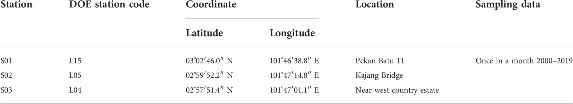
TABLE 1. Coordinates of selected sampling water quality monitoring station.

FIGURE 1

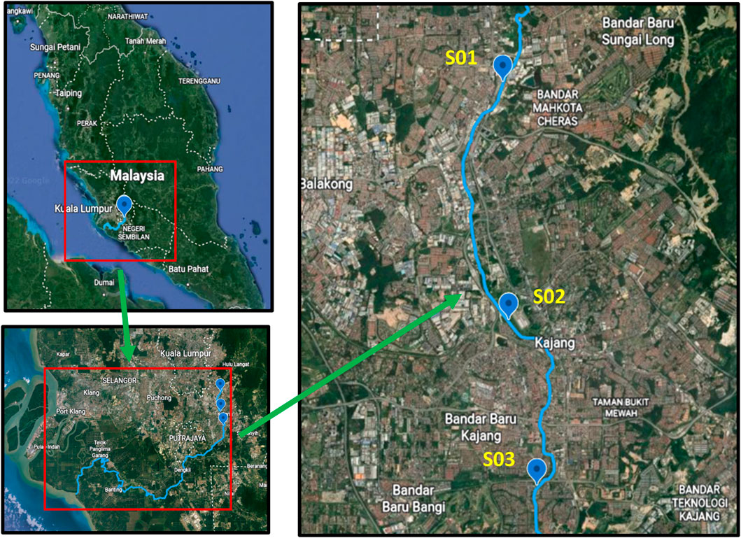
FIGURE 1. Water quality monitoring stations of the Langat River.

2.2 SVM model development

Given how important it is to protect the environment, the main goal of this study is to build an SVM model-based tool for predicting WQI and displaying measurement data in very specific phases. In this regard, the section will concentrate on constructing a prediction model for WQI with a reliable method by employing the SVM model to estimate the WQI without utilizing parameter indices, but rather by directly using physical values from parameters. The major advantage of this model is that the computation of WQI is possible especially when one or more of the parameters is missing. The following pre-processing steps were employed to enhance the prediction model in this study. Figure 2 depicts a summary of the processes followed to develop the prediction model for this study. During the various stages of model development, “R programming” is used as a tool for performing all analyzes (Karatzoglou et al., 2022; Meyer, 2022).

FIGURE 2

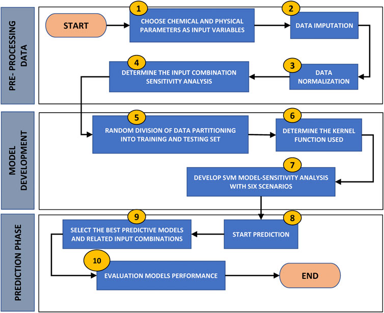
FIGURE 2. Overview of workflow to build the predictive model.

2.2.1 Data imputation

To begin, data imputation for water quality has been done, with the CART method used to impute and fill in data gaps. Missing data is an unavoidable occurrence in water quality monitoring systems (Hamzah et al., 2021). The bulk of data analysis techniques requires the input of comprehensive data sets (Pillai et al., 2019; Hadeed et al., 2020). Incomplete data might result in skewed or erroneous results, which can have a detrimental effect on the conclusions taken from data on water quality (Ratolojanahary et al., 2019). CART is an established machine learning classification technique (Mauro Assis Gomes et al., 2020) that utilizes the concept of classifiers and cut points in variables to split the sample. The sample was subsampled into broader, more homogeneous subsamples using cut points. In both subsamples, the splitting method is used more than once. This makes a binary tree with many splits (Rodríguez et al., 2021).

2.2.2 Water quality index

After imputation of the data, DOE-WQI is calculated and compared with the predicted SVM-WQI. The WQI is derived from water quality data and is used to determine the current status of a river’s water quality. Numerous variables must be considered when evaluating the degree of change in water quality. The WQI is an index that has no dimensions. It is composed of specific water quality parameters. The WQI provides a method for classifying water quality of water bodies both in the past and in the present. The meaningful value of the WQI can influence the decisions and actions of policy makers. Water quality improves the higher the index value on a scale of 1–100. River stations that have a score of 80 or higher are generally classified as clean rivers because they meet water quality standards. Water quality is considered polluted when the WQI is below 40, while stations with a value between 40 and 80 mean that water quality is even slightly polluted (Yahya et al., 2019).

For more than 25 years, DOE has used a river WQI that includes six key water quality parameters: Dissolved oxygen (DO), biochemical oxygen demand (BOD), chemical oxygen demand (COD), pH, ammoniacal nitrogen (AN) and suspended solids (SS). The WQI is used as the basis for environmental assessment of a watercourse to classify pollution loads and establish classes of beneficial uses, as provided in INWQS. The formula for calculating the WQI is given in Eq. 1. In Eq. 1, DO has the highest weighting, while pH has the lowest weighting. Before calculating the WQI, each of the six parameters is first converted into a sub-index (SI) and the SIs are selected according to the mathematical relationships that give the correct combination and are given in Eqs 2–18.

$\mathrm{D}\mathrm{O}\mathrm{E}-\mathrm{W}\mathrm{Q}\mathrm{I}=0.22\left(\mathrm{S}\mathrm{I}\mathrm{D}\mathrm{O}\right)+0.19\left(\mathrm{S}\mathrm{I}\mathrm{B}\mathrm{O}\mathrm{D}\right)+0.16\left(\mathrm{S}\mathrm{I}\mathrm{C}\mathrm{O}\mathrm{D}\right)+0.15\left(\mathrm{S}\mathrm{I}\mathrm{A}\mathrm{N}\right)+0.16\left(\mathrm{S}\mathrm{I}\mathrm{S}\mathrm{S}\right)+0.12\left(\mathrm{S}\mathrm{I}\mathrm{p}\mathrm{H}\right)(1)$

$\mathrm{S}\mathrm{u}\mathrm{b}-\mathrm{i}\mathrm{n}\mathrm{d}\mathrm{e}\mathrm{x}\mathrm{D}\mathrm{O}\left(\%\mathrm{s}\mathrm{a}\mathrm{t}\mathrm{u}\mathrm{r}\mathrm{a}\mathrm{t}\mathrm{i}\mathrm{o}\mathrm{n}\right):$

$\mathrm{x}\le 8,\mathrm{S}\mathrm{I}\mathrm{D}\mathrm{O}=0(2)$

$\mathrm{x}\ge 92,\mathrm{S}\mathrm{I}\mathrm{D}\mathrm{O}=100(3)$

$8<\mathrm{x}<92,\mathrm{S}\mathrm{I}\mathrm{D}\mathrm{O}=-0.395+0.03{\mathrm{x}}^2-0.0002{\mathrm{x}}^3(4)$

$\mathrm{S}\mathrm{u}\mathrm{b}-\mathrm{i}\mathrm{n}\mathrm{d}\mathrm{e}\mathrm{x}\mathrm{B}\mathrm{O}\mathrm{D}\left(\mathrm{m}\mathrm{g}/\mathrm{L}\right):$

$\mathrm{x}\le 5,\mathrm{S}\mathrm{I}\mathrm{B}\mathrm{O}\mathrm{D}=100.4-4.23\mathrm{x}(5)$

$\mathrm{x}>5,\mathrm{S}\mathrm{I}\mathrm{B}\mathrm{O}\mathrm{D}=108^{-0.055\mathrm{x}}-0.1\mathrm{x}(6)$

$\mathrm{S}\mathrm{u}\mathrm{b}-\mathrm{i}\mathrm{n}\mathrm{d}\mathrm{e}\mathrm{x}\mathrm{C}\mathrm{O}\mathrm{D}\left(\mathrm{m}\mathrm{g}/\mathrm{L}\right):$

$\mathrm{x}\le 20,\mathrm{S}\mathrm{I}\mathrm{C}\mathrm{O}\mathrm{D}=-1.33\mathrm{x}+99.1(7)$

$\mathrm{x}>20,\mathrm{S}\mathrm{I}\mathrm{C}\mathrm{O}\mathrm{D}=103{\mathrm{e}}^{-0.0157\mathrm{x}}-0.04\mathrm{x}(8)$

$\mathrm{S}\mathrm{u}\mathrm{b}-\mathrm{i}\mathrm{n}\mathrm{d}\mathrm{e}\mathrm{x}\mathrm{A}\mathrm{N}\left(\mathrm{m}\mathrm{g}/\mathrm{L}\right):$

$\mathrm{x}\le 0.3,\mathrm{S}\mathrm{I}\mathrm{A}\mathrm{N}=100.5-105\mathrm{x}(9)$

$0.3<\mathrm{x}<4,\mathrm{S}\mathrm{I}\mathrm{A}\mathrm{N}=94{\mathrm{e}}^{-0.573\mathrm{x}}-5\left|\mathrm{x}-2\right|(10)$

$\mathrm{x}\ge 4,\mathrm{S}\mathrm{I}\mathrm{A}\mathrm{N}=0(11)$

$\mathrm{S}\mathrm{u}\mathrm{b}-\mathrm{i}\mathrm{n}\mathrm{d}\mathrm{e}\mathrm{x}\mathrm{S}\mathrm{S}\left(\mathrm{m}\mathrm{g}/\mathrm{L}\right):$

$\mathrm{x}\le 100,\mathrm{S}\mathrm{I}\mathrm{S}\mathrm{S}=97.5{\mathrm{e}}^{-0.00676\mathrm{x}}+0.05\mathrm{x}(12)$

$100<\mathrm{x}<1000,\mathrm{S}\mathrm{I}\mathrm{S}\mathrm{S}=71{\mathrm{e}}^{-0.0061\mathrm{x}}-0.015\mathrm{x}(13)$

$\mathrm{x}\ge 1000,\mathrm{S}\mathrm{I}\mathrm{S}\mathrm{S}=0(14)$

$\mathrm{S}\mathrm{u}\mathrm{b}-\mathrm{i}\mathrm{n}\mathrm{d}\mathrm{e}\mathrm{x}\mathrm{p}\mathrm{H}:$

$\mathrm{x}<5.5,\mathrm{S}\mathrm{I}\mathrm{p}\mathrm{H}=17.02-17.2\mathrm{x}+5.02{\mathrm{x}}^2(15)$

$\mathrm{x}<7,\mathrm{S}\mathrm{I}\mathrm{p}\mathrm{H}=-242+95.5\mathrm{x}-6.67{\mathrm{x}}^2(16)$

$\mathrm{x}<8.75,\mathrm{S}\mathrm{I}\mathrm{p}\mathrm{H}=-181+82.4\mathrm{x}-6.05{\mathrm{x}}^2(17)$

$\mathrm{x}\ge 8.75,\mathrm{S}\mathrm{I}\mathrm{p}\mathrm{H}=536-77\mathrm{x}+2.76{\mathrm{x}}^2(18)$

2.2.3 Data normalization

After DOE-WQI done computed, the water quality parameters and DOE-WQI data were then normalized using the min-max method to avoid overfitting and ensure the accuracy of the results due to the scale differences between the various water quality parameters, and the data normalization is essential when dealing with attributes with varying scales, as this may result in lesser effectiveness of a critical attribute (with a lower scale) due to the presence of other attributes with varying scales (Adeyemo et al., 2020). Additionally, the normalization of data helps accelerate the training process and lessen the impact of dataset outliers (Ho et al., 2019). Thus, after normalizing the dataset, the machine learning model’s efficiency increases. The strength of this approach is that it maintains the exact relationships between the data items. It performs exceptionally well and does not inject any potential bias into the data (Dong et al., 2019).

2.2.4 Data partitioning

Finally, data was partitioned for building the predictive model to optimize the model’s performance. The fundamental principle behind data partitioning is to exclude a subset of accessible data from analysis and utilize it afterward to verify the model. The data partition is utilized to avoid too optimistic model precision estimations. Data partitioning is typically used in conjunction with supervised learning approaches (e.g., SVM), in which a predictive model is chosen from a set of models based on their performance on the training set. In this study, 80% of the data were randomly classified for training purposes, while 20% were classified to test the results using a 10-fold cross-validation technique. Even though there is no broadly adopted formula for modelling temporal and spatial predictions, this ratio is the most utilized method (Bui et al., 2020; Ghorbani et al., 2021).

2.2.5 Regression in SVM

SVM, which was initially intended to handle the classification problem and is currently being expanded to address the regression challenge (Ling et al., 2019). The training points closest to the separating hyperplane are the support vectors. There are responsible decision functions, such as hyperplanes that can denote the positive and negative data that has defined the maximum margins. This indicates that the distance between the nearest positive sample and the hyperplane should be minimized, while the distance between the nearest negative sample and the hyperplane should be maximized (Yahya et al., 2019). The kernel function has the most significant impact on SVM model prediction compared to other factors like scale factor and regulation parameter. The regression model employs the function defined in Eq. 19:

$\mathit{y}\left(\mathit{x}\right)={\mathit{w}}^{\mathit{T}}\mathit{\varphi }\left(\mathit{x}\right)+\mathit{b}(19)$

here, ϕ(x) can be any nonlinear kernel function (including the polynomial, radial basis, linear and sigmoid) and the weight (w) and bias vectors (b) values derived from the training data set. Estimation of coefficients w and b is performed by minimizing the sum of the empirical risk and a complexity component, whereas SVM regression is performed in feature space with high dimensions through a nonlinear mapping. Iterative trial-and-error calibration was implemented to determine the type of kernel function to employ and the value of the regularization parameter. SVM regression is categorized into two categories. Epsilon regression, often known as Type 1, or Nu regression, is the second type of regression (Behmel et al., 2016). For more details, readers may refer to Mamat et al. (2021) to get a better grasp of the structure of the SVM.

To build a WQI prediction model using the regression component of the SVM model and water quality data, the following steps must be performed in sequence.

Step 1. Selection of the independent (predictor) and dependent (target response) variables.To determine whether the SVM regression model is capable of learning the behavior of the WQI used by Malaysian DOE, six water quality parameters (DO, BOD, COD, pH, AN, SS) originally used to calculate the WQI based on Eq. 1 were selected as input predictors (x) and the WQI as the target response (y) in this study.

Step 2. Train the SVM regression model with the training set.When developing a machine learning model, the data must always be divided into a training set and a testing set. The SVM model is trained using the values from the training set and the WQI is predicted and evaluated using the testing set.

Step 3. Determine the kernel function and set up the parameters for the training setThe first goal of this part is to determine the kernel functions that best fit the SVM model that can be used to predict the WQI. The kernel functions include linear, radial basis, polynomial, and sigmoidal kernel functions. The same training data is used four times to train the model for four different kernel functions. After analyzing the performance of the four models, it is determined which kernel has the best fitting kernel function. The optimal kernel function is then used to train the tuning parameters of the SVM model. To obtain valid predictive performance for the SVM model, the optimal parameter settings must be carefully selected because they all affect the generalization performance of the SVM model. During the training phase of the SVM simulation, the parameters are calibrated by trial and error and multiple test runs. During the testing phase, the WQI prediction model is configured with the optimal parameters.

Step 4. Predicting the results from the testing set.In this step, the WQI is predicted from the testing set using the SVM model developed for unseen data.

Step 5. Comparison of the testing set with the predicted values.For performance comparisons, the WQI values from the testing set are displayed as ‘observed’, while the WQI values predicted by the SVM are displayed as ‘predicted’.

Step 6. Visualization of the SVM resultsIn this step, the ‘observed’ and ‘predicted’ WQI are plotted to visualize the results and performance.

Step 7. Prediction of the WQI using the SVM model and sensitivity analysisAfter reducing the possible combinations of input predictors from the original set of six established in Step 1, Steps 6 through 8 are performed again for sensitivity analysis for each of Scenarios two through 6.

2.2.6 Sensitivity analysis of various modelling scenarios

A sensitivity analysis of a developed model evaluates the uncertainties between a model’s predictions and its input parameters. As part of the process of establishing the model, all six water quality measures were utilized as input variables to assess the model’s effectiveness. There are three main purposes of this research which are mainly to utilize the SVM model as an alternative efficient method to predict WQI. The first scenario was run using all six parameters as input variables which serve as a reference model by avoiding the calculation of sub-indices and directly using raw physical values of parameters. Second, to demonstrate that the model can estimate WQI even with missing parameters, a sensitivity analysis was conducted by omitting one of the six parameters. The SVM performance model was then tested using all the model performance criteria used for this study to assess the significance of the input parameters of the first scenario model. Moreover, sensitivity analysis was very useful and reliable when sufficient data were available to assess the relative importance of the parameter (Bui et al., 2020). Third, this predictive modelling puts a lot of emphasis on how accurate predictions are when they are based on a small number of input characteristics. This makes it easier and faster to discover the WQI of a river. Each scenario was made by reducing the model input parameters from the six parameters required by the DOE to five, four, three, two, and one parameter. Implementing the proposed support vector machine model with a minimum number of model input variables would result in a low cost for river WQI prediction. This might also reduce the time required to analyze a water sample in the lab to determine the break-off parameters. The third scenario contains four inputs, resulting in five possible water quality parameter configurations. In the fourth scenario, there are three inputs, in the fifth scenario there are two inputs, and in the sixth scenario there is just one water quality indicator considered. Table 2 show all possible efficient combinations of input parameters for six different scenarios.

TABLE 2

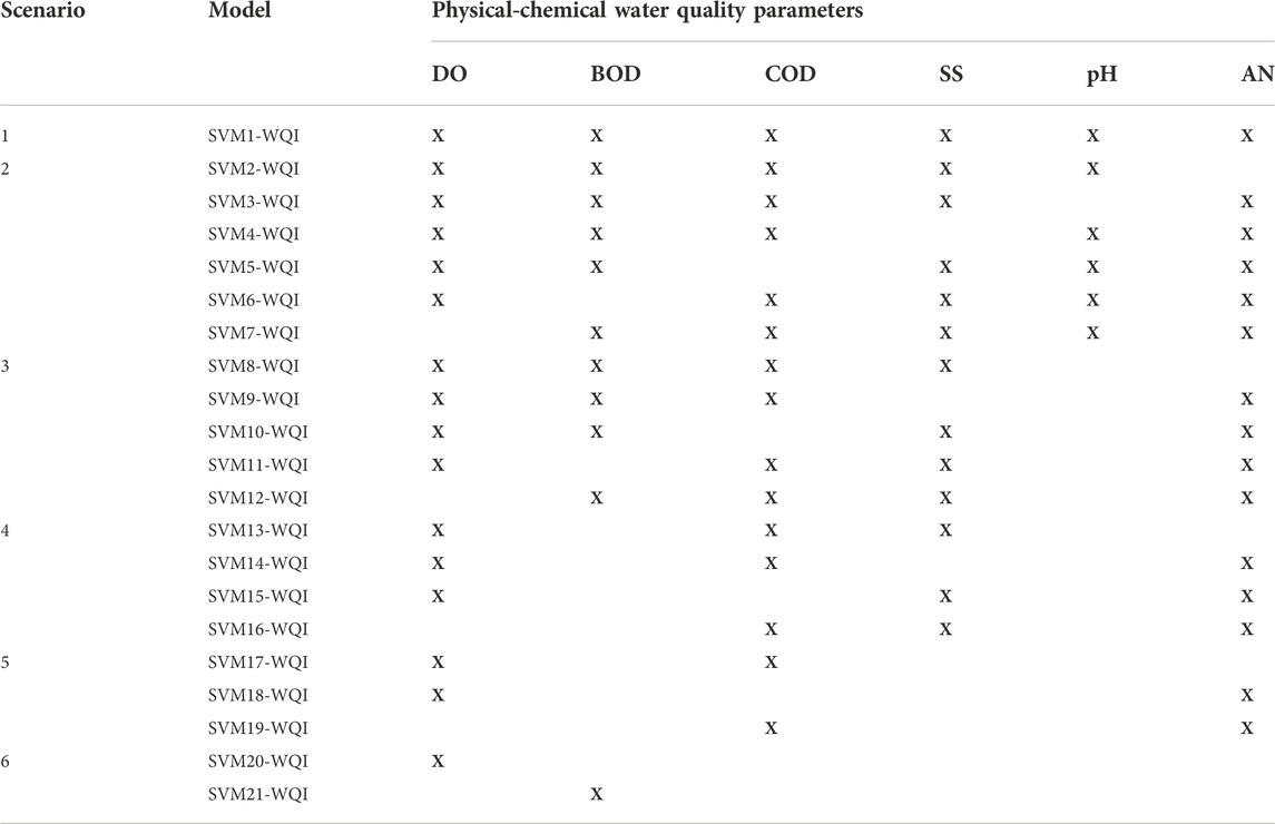
TABLE 2. Input combination data for each scenario in sensitivity analysis, with the considered parameter is marked with “X”.

2.3 Evaluation indicators

Several key metrics were utilized to assess the performance of the prediction models. Comparing predicted and observed data helped identify the optimal estimation WQI model. MAE, r, NSE, WI, and PBIAS were used to compare the accuracy of the deployed models in estimating WQI. The objective function was chosen as NSE since it is the most constraining (Narbondo et al., 2020). MAE and r were utilized for estimation, whereas WI and PBIAS were employed for validation.

2.3.1 Mean absolute error (MAE)

The mean difference between predicted and actual data is defined as a mean absolute error (Avila et al., 2018). The MAE ranges from 0 to infinity, with 0 being the best fit. Some researchers suggest using MAE instead of RMSE (Moriasi et al., 2015; Willmott et al., 2017). MAE is more interpretable than root mean square error (RMSE). In mathematics, MAE is the average absolute difference between two variables. MAE is easier to understand than the average of squared errors. Moreover, unlike RMSE, each error affects MAE proportionally to its absolute value.

$\mathit{M}\mathit{A}\mathit{E}=\frac{1}{\mathit{n}}{\displaystyle \sum }_{\mathit{i}=1}^{\mathit{n}}\left|{{\mathit{y}}_{\mathit{i}}}^{\mathit{o}\mathit{b}\mathit{s}\mathit{e}\mathit{r}\mathit{v}\mathit{e}\mathit{d}}-{{\mathit{y}}_{\mathit{i}}}^{\mathit{p}\mathit{r}\mathit{e}\mathit{d}\mathit{i}\mathit{c}\mathit{t}\mathit{e}\mathit{d}}\right|(20)$

2.3.2 Pearson correlation coefficient (r)

Pearson correlation coefficient, r measures the degree and direction of the linear connection between actual and predicted data. The values might vary between -1 and 1, inclusive. r usually appears to be the most effective and straightforward method for evaluating variable combinations related to water quality (Asadollah et al., 2021).

$\mathit{r}=\frac{{\displaystyle \sum }_{\mathit{i}=1}^{\mathit{n}}\left({\mathit{y}}_{\mathit{i}}^{\mathit{o}\mathit{b}\mathit{s}\mathit{e}\mathit{r}\mathit{v}\mathit{e}\mathit{d}}-{\overline{\mathit{y}}}^{\mathit{o}\mathit{b}\mathit{s}\mathit{e}\mathit{r}\mathit{v}\mathit{e}\mathit{d}}\right)\left({\mathit{y}}_{\mathit{i}}^{\mathit{p}\mathit{r}\mathit{e}\mathit{d}\mathit{i}\mathit{c}\mathit{t}\mathit{e}\mathit{d}}-{\overline{\mathit{y}}}^{\mathit{p}\mathit{r}\mathit{e}\mathit{d}\mathit{i}\mathit{c}\mathit{t}\mathit{e}\mathit{d}}\right)}{\sqrt{{\displaystyle \sum }_{\mathit{i}=1}^{\mathit{n}}{\left({\mathit{y}}_{\mathit{i}}^{\mathit{o}\mathit{b}\mathit{s}\mathit{e}\mathit{r}\mathit{v}\mathit{e}\mathit{d}}-{\overline{\mathit{y}}}^{\mathit{o}\mathit{b}\mathit{s}\mathit{e}\mathit{r}\mathit{v}\mathit{e}\mathit{d}}\right)}^2{\displaystyle \sum }_{\mathit{i}=1}^{\mathit{n}}{\left({\mathit{y}}_{\mathit{i}}^{\mathit{p}\mathit{r}\mathit{e}\mathit{d}\mathit{i}\mathit{c}\mathit{t}\mathit{e}\mathit{d}}-{\overline{\mathit{y}}}^{\mathit{p}\mathit{r}\mathit{e}\mathit{d}\mathit{i}\mathit{c}\mathit{t}\mathit{e}\mathit{d}}\right)}^2}}(21)$

2.3.3 Nash Sutcliffe efficiency (NSE)

The NSE was used to evaluate the performance of the model. As a normalized statistic, the NSE determines how much ‘noise’ is present compared to how much ‘information’ is present in the data of an experiment (Moriasi et al., 2015). In terms of NSE, the NSE is a measure of how well the observed and estimated data plots match the 1:1 line. NSE is between -∞ and 1.0 (including 1), with NSE = 1 being the optimal value. Performance levels between 0.0 and 1.0 are generally considered acceptable, but values below 0.0 indicate a poorer correlation between observed and predicted values, indicating poor performance.

$\mathit{N}\mathit{S}\mathit{E}=1-\frac{{\displaystyle \sum }_{\mathit{i}=1}^{\mathit{n}}\left({\mathit{y}}_{\mathit{i}}^{\mathit{o}\mathit{b}\mathit{s}\mathit{e}\mathit{r}\mathit{v}\mathit{e}\mathit{d}}-{\mathit{y}}_{\mathit{i}}^{\mathit{p}\mathit{r}\mathit{e}\mathit{d}\mathit{i}\mathit{c}\mathit{t}\mathit{e}\mathit{d}}\right)}{{\displaystyle \sum }_{\mathit{i}=1}^{\mathit{n}}\left({\mathit{y}}_{\mathit{i}}^{\mathit{o}\mathit{b}\mathit{s}\mathit{e}\mathit{r}\mathit{v}\mathit{e}\mathit{d}}-{\overline{\mathit{y}}}^{\mathit{o}\mathit{b}\mathit{s}\mathit{e}\mathit{r}\mathit{v}\mathit{e}\mathit{d}}\right)}(22)$

2.3.4 Willmott’s index of agreement (WI)

Willmott introduced the agreement index (WI) as a standard method for assessing the extent of model prediction error. It is calculated by dividing the ‘potential error’ by the ‘mean square error’. It can incorporate measurement uncertainty (Martín et al., 2017).

$\mathit{W}\mathit{I}=1-\frac{{\displaystyle \sum }_{\mathit{i}=1}^{\mathit{n}}{\left({\mathit{y}}_{\mathit{i}}^{\mathit{o}\mathit{b}\mathit{s}\mathit{e}\mathit{r}\mathit{v}\mathit{e}\mathit{d}}-{\mathit{y}}_{\mathit{i}}^{\mathit{p}\mathit{r}\mathit{e}\mathit{d}\mathit{i}\mathit{c}\mathit{t}\mathit{e}\mathit{d}}\right)}^2}{{\displaystyle \sum }_{\mathit{i}=1}^{\mathit{n}}{\left(\left|{\mathit{y}}_{\mathit{i}}^{\mathit{p}\mathit{r}\mathit{e}\mathit{d}\mathit{i}\mathit{c}\mathit{t}\mathit{e}\mathit{d}}-{\overline{\mathit{y}}}^{\mathit{o}\mathit{b}\mathit{s}\mathit{e}\mathit{r}\mathit{v}\mathit{e}\mathit{d}}\right|+\left|{\mathit{y}}_{\mathit{i}}^{\mathit{o}\mathit{b}\mathit{s}\mathit{e}\mathit{r}\mathit{v}\mathit{e}\mathit{d}}-{\overline{\mathit{y}}}^{\mathit{o}\mathit{b}\mathit{s}\mathit{e}\mathit{r}\mathit{v}\mathit{e}\mathit{d}}\right|\right)}^2}(23)$

2.3.5 Percent bias (PBIAS)

The percentage bias metric (PBIAS) quantifies the average probability that the simulated data is greater or less than the observed data. PBIAS is ideally 0.0, with low values indicating efficient model simulation. Positive numbers indicate an overestimation of the model, while negative values indicate an underestimation of the model (Moriasi et al., 2015). PBIAS is the deviation of the data analyzed, represented as a percentage of the mean.

$\mathit{P}\mathit{B}\mathit{I}\mathit{A}\mathit{S}=\left[\frac{{\displaystyle \sum }_{\mathit{i}=1}^{\mathit{n}}\left({\mathit{y}}_{\mathit{i}}^{\mathit{o}\mathit{b}\mathit{s}\mathit{e}\mathit{r}\mathit{v}\mathit{e}\mathit{d}}-{\mathit{y}}_{\mathit{i}}^{\mathit{p}\mathit{r}\mathit{e}\mathit{d}\mathit{i}\mathit{c}\mathit{t}\mathit{e}\mathit{d}}\right)}{{\displaystyle \sum }_{\mathit{i}=1}^{\mathit{n}}\left({\mathit{y}}_{\mathit{i}}^{\mathit{o}\mathit{b}\mathit{s}\mathit{e}\mathit{r}\mathit{v}\mathit{e}\mathit{d}}\right)}*\left(100\right)\right](24)$

The following table contains the standard review of performance values and ratings for NSE, WI, and PBIAS used in this work, as indicated in Table 3 (Moriasi et al., 2015; Rodríguez et al., 2021).

TABLE 3

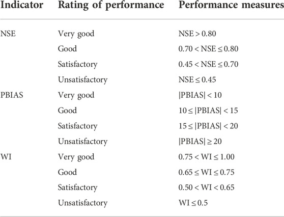
TABLE 3. Evaluation indicators and associated rating of performance.

3 Results and discussion

Developing the optimal SVM model will be discussed in detail further down. The Malaysian DOE provided the data for the water quality analysis in this study. For SVM modelling, this work used monthly time series data sets for six chosen parameters (DO, BOD, COD, pH, SS, AN) from three locations from 2000 to 2019.

3.1 SVM model development

This study’s initial goal is to identify the kernel functions that best fit the SVM model for WQI and can be utilized to predict WQI. Table 4 shows the results of the model prediction analysis for several kernel function types, including Linear, Radial Basis or Gaussian, Polynomial, and Sigmoidal kernel functions. The RBF kernel function has the highest correlation coefficient (0.990, 0.989) during the training and testing phases, followed by linear (0.951, 0.978), polynomial (0.904, 0.890), and sigmoid kernel functions (0.321, 0.904). As a result, the RBF kernel function will be employed for further development.

TABLE 4

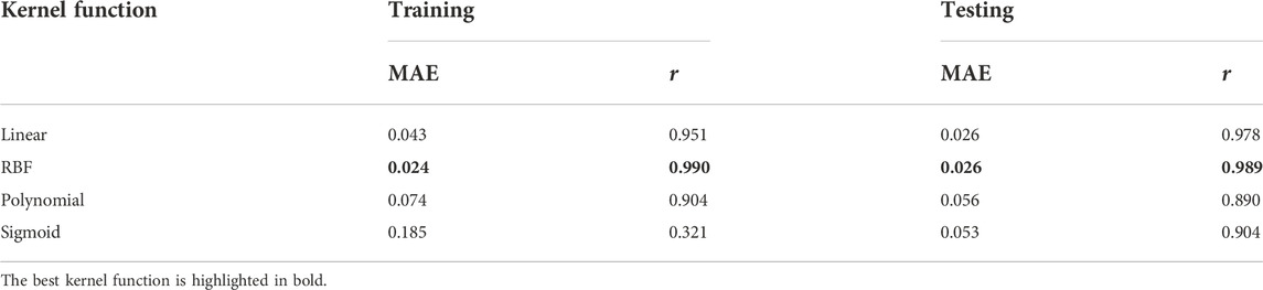
TABLE 4. Performance of SVM model with four kernel functions.

To achieve valid predictive performance for the SVM model, the optimal parameter sets must be carefully chosen since they all have an impact on SVM generalization performance. Therefore, for the next part, two types of RBF kernel functions, Epsilon and Nu, are trained to determine the best SVM efficiency for WQI prediction. Based on the results of the 10-fold cross-validation, the optimal architecture of the SVM model was chosen. K-fold CV is a robust technique for evaluating model accuracy. In terms of 10-fold CV value, Table 5 shows that the Nu-RBF model outperforms the Epsilon-RBF model. According to this data, the error variance between actual and predicted WQI values is extremely small. This also demonstrates how effective the combination of Nu-RBF and 10-fold CV model selection is.

TABLE 5

TABLE 5. Performance of RBF kernel functions.

Aside from that, there are two crucial factors to consider: the gamma and capacity parameters. These elements are critical for optimizing the structure of the SVM model that will be used in these situations. During the training phase of the SVM simulation, the gamma and capacity parameters, were calibrated using several tests runs and trial and error. The optimal gamma and capacity parameters to use for the WQI prediction model during training and testing are capacity = 6 and gamma = 0.5. As a result, the SVM model with a hybrid of Nu-RBF (capacity = 6 and gamma = 0.5) and 10-fold CV is chosen as an effective final prediction model.

3.2 Sensitivity analysis of SVM modelling scenarios

In Malaysia, the DOE developed the WQI formula based on the INWQS, which uses six water quality parameters (ammoniacal nitrogen (AN), biochemical oxygen demand (BOD), chemical oxygen demand (COD), dissolved oxygen (DO), pH, and suspended solids (SS)). One of the primary constraints of DOE-WQI is that if any of the six parameters are missing, the calculation of DOE-WQI is impossible to proceed with. To obtain actual or near-actual values for river water, this study offered the data-driven SVM-WQI model to solve this problem using all six parameters or a minimal number of parameters. Sensitivity analysis with six different scenarios is evaluated in this study to determine the best combination for WQI prediction. In both the training and testing phases, the accuracy of the models is assessed using statistical indices such as MAE, r, NSE, WI, and PBIAS. A testing dataset was used to evaluate the models, and the most effective one was chosen for modeling and further study. This result merely reveals how well the models match the training dataset, as all models were constructed using the training dataset. The training data were not used for model evaluation. An evaluation was conducted utilizing testing data (Bui et al., 2020). From the findings as well, it can generally be noticed that the prediction performance is higher in the training phase than in the testing phase. This is to be expected because the prediction error is minimized during the training phase, and the model built during the training phase is tested during the testing phase (Yahya et al., 2019).

Before performing the sensitivity analysis, it is necessary to examine the relationship between the six input parameters and the WQI to determine the combination that provides the most accurate prediction of the WQI. Table 6 shows the values of the Pearson correlation matrix between the different input parameters considered and the WQI. When evaluating the different possible combinations of input variables, the Pearson correlation coefficient method consistently proves to be the most effective and easiest to understand (Malik et al., 2020; Sharafati et al., 2020; Asadollah et al., 2021). According to Table 6, DO has the strongest correlation with WQI, while pH has the weakest correlation. It is also interesting to note that biochemical oxygen demand (BOD) is the second strongest correlated parameter with water quality index (WQI). The results shown in Table 6 are used in selecting the different input parameter combinations for WQI prediction, with the goal of gradually eliminating parameters that have lower Pearson correlation with WQI. As you can see from Tables 7, 8, 9, 10, 11, 12, a total of twenty-one different combinations of input parameters were considered (SVM1 to SVM21).

TABLE 6

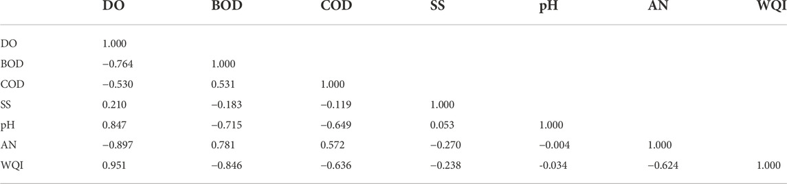
TABLE 6. Correlation matrix between selected water quality parameters and the WQI.

TABLE 7

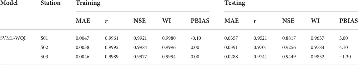
TABLE 7. Performance evaluations for the first scenario.

TABLE 8

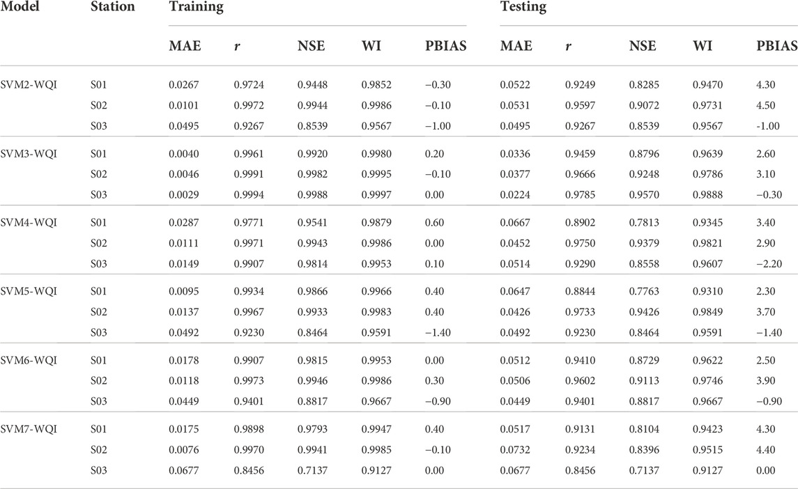
TABLE 8. Performance evaluations for the second scenario.

TABLE 9

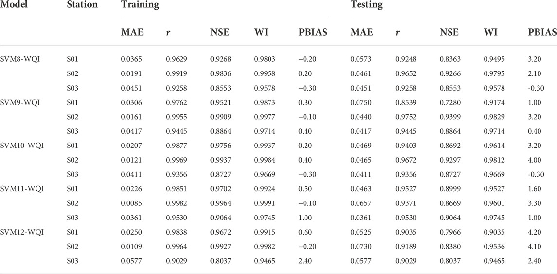
TABLE 9. Performance evaluations for the third scenario.

TABLE 10

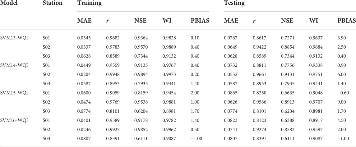
TABLE 10. Performance evaluations for the fourth scenario.

TABLE 11

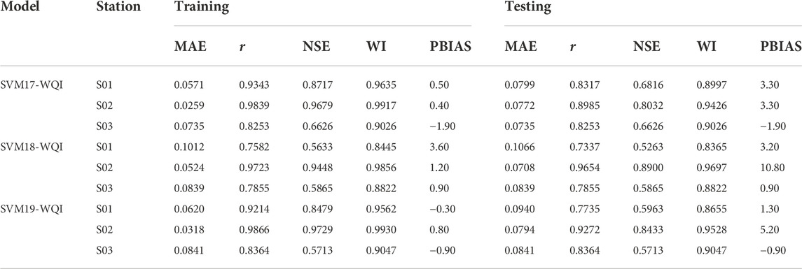
TABLE 11. Performance evaluations for the fifth scenario.

TABLE 12

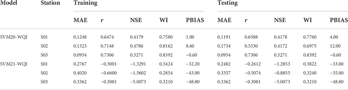
TABLE 12. Performance evaluations for the sixth scenario.

3.2.1 First scenario: Originally with all six parameters

In the first scenario, the SVM1-WQI has been trained and tested with the six originally defined input parameters that have been used in DOE-WQI. The main goal to achieve in this scenario is to develop an alternative model that can predict WQI with high accuracy and stability by using direct measured physical values without sub-index calculation within WQI equations. The results of the SVM1-WQI implementation for the different monitoring stations are shown in Table 7. It is clearly shown that in both phases, the model was exceptionally able to replicate the behavior of DOE-WQI and attained very high accuracy. The performance for model SVM1-WQI (Station S01: r_Train = 0.9961, MAE_Train = 0.0047, r_Test = 0.9521, MAE_Test = 0.0357; Station S02: r_Train = 0.9992, MAE_Train = 0.0038, r_Test = 0.9701, MAE_Test = 0.0391; Station S03: r_Train = 0.9989, MAE_Train = 0.0046, r_Test = 0.9741, MAE_Test = 0.0288). The lowest value of MAE signifies the high model robustness along with the highest degree of r, NSE, WI, and PBIAS. SVM1-WQI has a high degree of precision and minimal residual error. Figures 3A, 4A which depict a time series plot and a scatter plot, respectively, reflect this agreement. Figure 3A depicts a comparison of the actual (DOE-WQI) and predicted (SVM1-WQI) values for Station S03 using the chosen Nu-RBF model. The vertical axis represents WQI data, and the horizontal axis represents time set. The plot shows that the SVM1-WQI model is capable of predicting WQI. This capability is visualized by the similarity behavior of the plot between the actual and predicted values of WQI. The closeness of this data indicates that the deviation of error is very small and can be neglected. The association of SVM1-WQI for Station S03 has been plotted in Figure 4A. The vertical axis represents predicted WQI, and the horizontal axis represents actual WQI. The scatter plot graphically illustrates the association between the predicted and observed values of WQI. In the diagram, the line of the best fit is drawn as a reference and to describe the closeness of the relationship between the predicted and the observed data. As expected, SVM1-WQI shows excellent prediction performance as the data points are very close to the best fit line in the testing phase. Moreover, since SVM1-WQI is identical to the usual DOE-WQI technique, the first scenario, which includes all six parameters, was used as a standard benchmark for which other scenarios could be evaluated.

FIGURE 3

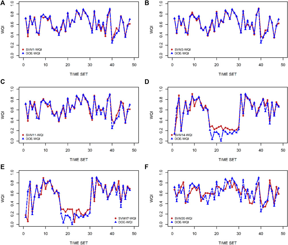
FIGURE 3. Comparison of the observed (DOE-WQI) and the best predicted model (SVM-WQI) for each scenario: (A) SVM1-WQI; (B) SVM3-WQI; (C) SVM11-WQI; (D) SVM14-WQI; (E) SVM17-WQI; and (F) SVM20-WQI.

FIGURE 4

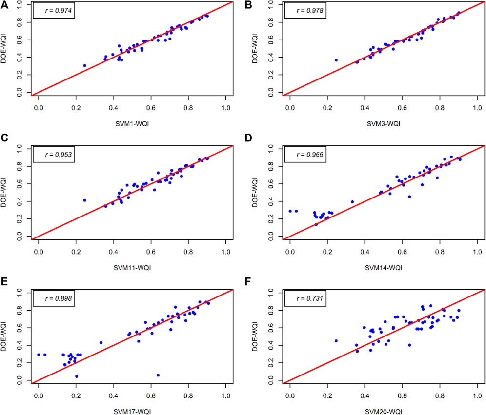
FIGURE 4. Correlation between the observed (DOE-WQI) and the best predicted model (SVM-WQI) for each scenario: (A) SVM1-WQI; (B) SVM3-WQI; (C) SVM11-WQI; (D) SVM14-WQI; (E) SVM17-WQI; and (F) SVM20-WQI.

3.2.2 Second scenario: Input data with five parameters

In the second scenario, the prediction model was run based on five different water quality parameters with six different combinations as shown in Table 8. The statistical indicators demonstrate the SVM model’s capacity to predict the WQI even without the original six parameters, with a high degree of accuracy (r, NSE, and WI criteria), all of which are more than 0.9. Furthermore, as can be seen in Table 8, among all the results for scenario 2, model SVM3-WQI offers better-quality estimates of WQI than the remaining models do. According to the displayed results, SVM3-WQI achieves the highest prediction accuracy during both the training and testing phases. The model SVM3-WQI is the combination of DO, BOD, COD, SS, and AN, excluding the pH parameter, with corresponding results (Station S01: r_Train = 0.9961, MAE_Train = 0.0040, r_Test = 0.9459, MAE_Test = 0.0336; Station S02: r_Train = 0.9991, MAE_Train = 0.0046, r_Test = 0.9666, MAE_Test = 0.0377 and Station S03: r_Train = 0.9994, MAE_Train = 0.0029, r_Test = 0.9785, MAE_Test = 0.0224). This model is highly affecting the estimated values of WQI. As a next step, all the possible combinations from SVM2-WQI to SVM7-WQI are simulated, and the results are listed in Table 8. In this predictive modelling, the effects of each water quality parameter were studied based on the analysis. In contrast, when DO is eliminated from the study, WQI yields the lowest accuracy. SVM7-WQI findings demonstrate the lowest accuracy (Station S01: r_Train = 0.9898, MAE_Train = 0.0175, r_Test = 0.9131, MAE_Test = 0.0517; Station S02: r_Train = 0.9970, MAE_Train = 0.0076, r_Test = 0.9234, MAE_Test = 0.0732 and Station S03: r_Train = 0.8456, MAE_Train = 0.0677, r_Test = 0.8456, MAE_Test = 0.0677). This discovery is extremely significant because it demonstrates that DO cannot be excluded from the study without compromising WQI’s overall performance. In the current WQI computation, the sub-index of DO includes a lengthy process in which the DO concentration must first be converted to % saturation, and then it must correspond with the sample day’s temperature (Fondriest Environmental, 2013). Without temperature information, the computation of the sub-index of DO and WQI would deteriorate. Remarkably, SVM1-WQI is able to circumvent this obstacle by adopting direct physical DO concentration. Furthermore, pH has been demonstrated to have a weak relationship with WQI prediction. In Malaysia, the pH of the water flowing into rivers is closely monitored. It is the easiest parameter to measure because it can be easily measured on-site and does not require to be tested in a lab. In addition, as Malaysia is a tropical country that experiences a significant amount of rainfall every year, the rain may readily dilute and neutralize the pH level in the rivers. Therefore, the lack of pH from the data used to generate predictions has little to no effect on how WQI is predicted. All quantitative results were in agreement with the research results obtained by Othman et al. (2020). It shows a strong correlation between the input parameters and the target response, WQI. The accuracy of the model performance generated by SVM3-WQI was only shown for Station S03 using the time series plot and scatter plot in Figure 3B shows the comparison of the actual DOE-WQI and SVM3-WQI. Meanwhile, Figure 4B displays the association between predicted and observed WQI values visually. The y-axis represents the actual DOE-WQI, whereas the x-axis represents the predicted SVM3-WQI. The line of best fit is drawn as a reference to describe the closeness of the correlation between the predicted and observed data in the plot. In the testing phase, SVM3-WQI makes great predictions (points close to the best fit line) for the Station S03.

Next, the primary objective of executing Scenarios three through six is to enhance model performance by minimizing the combination of input variables to the prediction model. The performance of the models is displayed in Figures 3C–F, 4C–F for the following scenarios. For the NSE assessment, the prediction results are generally considered “good”. The WQI predicted at the three monitoring sites provided the best estimate with a ‘good’ performance for all models assessed. The validation of the models was exceptional and gave ‘very good’ results for the assessments WI and PBIAS.

3.2.3 Third scenario: Input data with four parameters

Scenario three reduced the number of input variables by employing only four water quality factors for the model. Table 9 shows the results of an analysis of various input combinations. The water quality parameter combinations are considered after the model SVM3-WQI with the pH parameter omitted. By employing DO, COD, SS, and AN as inputs, SVM11-WQI achieves the optimum performance and prediction accuracy. Surprisingly, the accuracy of SVM10-WQI does not differ much from SVM11-WQI with combinations of DO, BOD, SS, and AN. Incidentally, BOD and COD are identical variables in both combinations. It is interesting to note that other combinations, such as SVM8-WQI, SVM9-WQI, and SVM12-WQI, nevertheless managed to hit the prediction accuracy benchmarks of r > 0.85, NSE >0.70, and WI > 0.90 across the stations. Compared to scenario 2, scenario three combines the deletion of pH with the elimination of other model inputs and produces a significant result for this predictive modelling that is close to scenario 2’s accuracy. Hence, all input combinations for the third scenario are qualified for this predictive modelling. The findings of the investigation carried out in the third scenario demonstrated that BOD is the parameter with the weakest correlation to the accurate predictions of WQI across all stations. There are a few challenges involved with BOD testing, including a 5-day incubation period, a long sample preparation method, and issues achieving reliable, repeatable findings. The major limitation of BOD analysis from an operational perspective is time lag. In addition, this scenario can determine which parameter correlates most significantly with WQI. Therefore, the exclusion of pH and BOD as predictive modelling inputs has the least impact on the prediction of WQI. SVM11-WQI, which eliminates pH and BOD from the predictive model, had the highest prediction accuracy across all five sets of possible combinations.

3.2.4 Fourth scenario: Input data with three parameters

In the fourth scenario, there were a total of three fewer inputs than in the previous scenario. This scenario is based on the best model SVM11-WQI from the third scenario which omitted the parameter of BOD, and pH, and with another parameter. Four potential combinations were analyzed using predictive modelling, and the findings are displayed in Table 10. With only three parameters, all models can predict WQI with a small prediction error (MAE) and strong statistical indicators of r > 0.80, NSE >0.60, and WI > 0.89 for all stations which are still in a good range of acceptable models to predict WQI. SVM14-WQI shows the best prediction accuracy with the combinations of DO, COD, and AN whilst those in SVM16-WQI are COD, SS and AN give the lowest accuracy. The fourth scenario showed that there is a weak relationship between SS and WQI prediction.

3.2.5 Fifth scenario: Input data with two parameters

In the fifth scenario, the input number has been further minimized to two variables. This scenario is based on the best model SVM14-WQI which excluded parameters of BOD, pH, and SS and with one more parameter. There are three different combinations were considered. Surprisingly, by using only two parameters to predict WQI, the results in Table 11 show that all models are still able to achieve outstanding prediction accuracy with low MAE and r > 0.75, NSE >0.56 and WI > 0.84 for all stations which are still in a range of satisfactory model to predict WQI. SVM17-WQI shows the best prediction accuracy with the combinations of DO and COD only whilst those in SVM18 are DO and AN give the lowest accuracy. The fifth scenario revealed that the association between AN and WQI prediction is the weakest. Again, in this instance, it is discovered that eliminating AN from the model reduces the model’s inaccuracy.

3.2.6 Sixth scenario: Input data with one parameter

Based on the best model in the fifth scenario, SVM17-WQI, just one parameter has to be evaluated for the sixth scenario, either DO or COD, which are SVM20-WQI and SVM21-WQI, respectively. Both DO and COD are chemical water quality indicators. According to all the statistical performance in Table 12, SVM20-WQI with low MAE, r > 0.53, NSE >0.56, and WI > 0.84 for all stations, which is still within the acceptable range for models to predict WQI, parameter DO is more accurate and gives a more acceptable value for predicting WQI than parameter COD. COD alone cannot provide sufficient precision for all stations to predict WQI. The sixth scenario demonstrated that DO concentration has a substantial effect on WQI prediction. This is not unexpected given that the vast majority of previously examined scenarios indicate that when DO is eliminated from the model, the model’s error will be large, and its accuracy will deteriorate. The significant DO parameter in WQI prediction can reveal information on the consequences of activities such as agricultural non-point sources and nearby animal farms along the river, as well as land development, on surface water quality.

3.3 Graphical performance comparisons of SVM modeling scenarios

In summary, the overall predictive performance of the best model from each scenario is visualized using scatter plots, boxplots, Taylor diagrams, and Violin plots. Scatter plots graphically illustrate the agreement between observed and predicted values, while boxplots show the performance indicators of the models. Taylor diagrams combine the root mean square error (RMSE), correlation coefficient (r), and standard deviation to visually identify the most accurate predictive model. Finally, Violin plots show the probability density function of the prediction results.

The most efficient method had the highest r and the lowest RMSE and MAE (Moriasi et al., 2015; Rodríguez et al., 2021). Consequently, the most accurate model for each scenario was selected and validated using the NSE, WI, and PBIAS formulas. The leading model for each scenario is shown in Tables 7, 8, 9, 10, 11, 12; the values derived by the performance evaluators and the corresponding score are shown in Table 3. In the NSE assessment, the minimum level of prediction performance is generally considered satisfactory, and the highest accuracy provided the best estimate with "very good" performance for all stations. The validation of the prediction model was exceptional and provided "very good" results for both the WI and PBIAS assessments.

Figure 5 shows a boxplot representation of the performance of the best models from all scenarios (r, NSE, WI, and PBIAS). There is a strong positive relationship between the predicted WQI and the combination of input parameters, with 0.99< r <0.70. While, NSE > 0.5 identifies 100% of the predicted WQI as "satisfactory" to "very good" and all predicted data having a positive NSE, indicating that the model outperformed the mean function used as an indicator for all predictions. The results of the validation were remarkable. In terms of the WI -score and the PBIAS scores, 100% of the predicted data are classified as "good’.

FIGURE 5

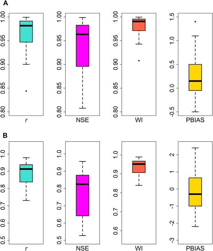
FIGURE 5. Boxplots for (A) the training phase and (B) the testing phase.

In addition, the models in the testing phase are also evaluated using Taylor diagrams (see Figure 6). As mentioned earlier, in a Taylor diagrams, r, standard deviation, and RSME are plotted, and the point corresponding to the model with the best predictive performance has the smallest distance from the “observed” point. Again, the Taylor diagrams show that in the test phase, the SVM1 and SVM3 models are characterized by the best predictive performance. Fortunately, the other fitted models are in the same reliable range as the predictive WQI model.

FIGURE 6

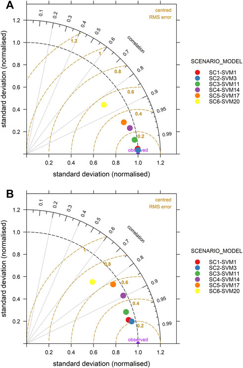
FIGURE 6. Normalized Taylor diagrams for (A) training phase and (B) testing phase.

Finally, Figure 7 compares the observed and predicted dispersion of WQI values in Violin plot diagrams and shows the probability density function with different quartiles (quartile-25%, quartile-50%, quartile-75%). The performance of the six best predictive models from each scenario is very similar, with the mean predicted and observed values not too far apart, indicating the same status of the WQI. According to the guidelines of DOE, a river with WQI values of 60–80 is considered slightly polluted (Department of Environment Malaysia, 2017). Moreover, the class of WQI predicted in each scenario in the Class III is the same as the observed class based on the INWQS. This confirms what has already been found with other means of visualizing predictive performance. All the best models have promising overall performance. The probability density function shapes further confirm this.

FIGURE 7

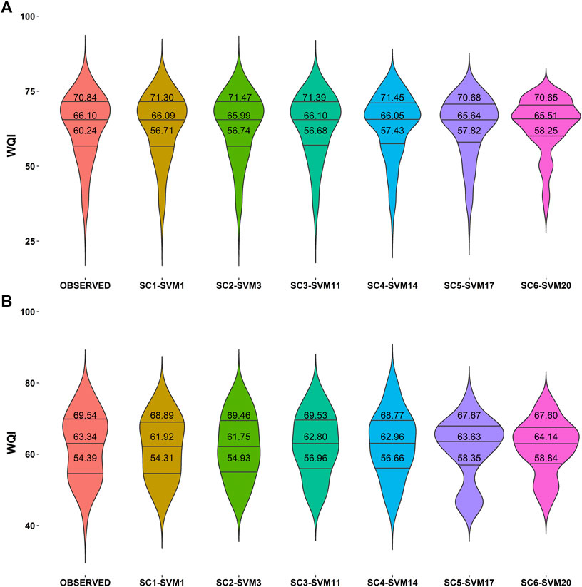
FIGURE 7. Violin plot of observed and predicted WQI values for (A) training phase and (B) testing phase.

4 Conclusion

Predicting the quality of water is crucial for pollution monitoring and compliance with water resource environmental standards. The complexity and variety of water quality throughout a watershed necessitate a reliable and adaptable WQI model to reduce the impact of nonlinearity and improve prediction performance. To predict WQI in the Langat River basin, a data-driven model with an SVM-based Nu-RBF algorithm with 10-fold cross-validation was employed in this work. Combining various input parameters resulted in the development of a six-scenario sensitivity analysis. The performance of twenty-one different models was compared. According to Bui et al. (2020), no model consistently performs better in every scenario. All models should be analyzed to discover which model performs optimally in which circumstances. Aside from the structure of a model, choosing the optimal combination of input variables is one of the most influential factors that affect performance. The following are the most significant conclusions of the study:

• The first scenario showed that the SVM model can easily imitate natural behavior and learn its nonlinearity by avoiding the calculation of sub-indices and instead using the raw physical values of parameters. It can do this while still getting a high WQI score.

• As a result of the second scenario, the statistical evaluator demonstrates the SVM model’s capacity to predict the WQI even without the original six parameters, with a high degree of accuracy (r, NSE, and WI criteria), all of which are greater than 0.9. The modelling process also revealed that the DO parameter is the most influential factor in determining WQI. It was subsequently followed by BOD and COD. The pH value is the least important determinant of WQI. A notable finding is that excluding DO from the model reduces overall WQI performance.

• In the third through fifth scenarios, it was discovered that applying various variable reduction combinations resulted in varying degrees of model performance and that the impacts of modifying the inputs on the models for this research area had inconsistent and divergent effects on modelling in other catchments, even when employing the same variable combinations. The models indicated that the variables with the greatest r > 0.8 and NSE >0.75 provide the most accurate predictions. The combination of factors with extremely low r and NSE has a detrimental effect on predictive ability.

• The proposed model SVM-based Nu-RBF algorithm is a dependable and economical way to improve surface water quality management. It is successful at predicting WQI by reducing the number of input variables with high accuracy. This model is likely to be much more beneficial in developing countries, where measuring some water quality parameters is expensive or may not be possible at all.

• This model has the potential to be implemented on other rivers with similar water quality and land use trends to enhance monitoring and environmental management.

• In the end, the model will greatly improve and expedite data-driven decision-making by making data more accessible and attainable without human interaction.

Data availability statement

The datasets presented in this article are not readily available because restrictions apply to the availability of these data. Data were obtained from the Department of Environmental Malaysia (DOE), Ministry of Natural Resources and Environment, Malaysia and are available with the permission of the Department of Environmental Malaysia (DOE), Ministry of Natural Resources and Environment, Malaysia. Requests to access the datasets should be directed to doe.gov.my.

Author contributions

In this article, three (3) authors contributed their ideas and works throughout the process to complete the article. The first author (NM) is the main provider for this article. She contributed the idea of the article, followed by writing the original draft, formal analysis, and submitting the article. The second author (SFMR) acted as the corresponding author and was responsible for the supervision, review, editing, and checking of the whole article. The third author (FBH) was responsible for reviewing, editing, and checking the entire article. All authors have read and agreed to the published version of the manuscript.

Acknowledgments

The authors would like to thank the Earth Observation Centre, Universiti Kebangsaan Malaysia, and the Department of Environmental Malaysia (DOE), Ministry of Natural Resources and Environment, Malaysia for providing the data for this research. This publication is supported by the Micro Grant Kolej Universiti Poly-Tech Mara and Universiti Kebangsaan Malaysia (GP-2021-K014876).

Conflict of interest

The authors declare that the research was conducted in the absence of any commercial or financial relationships that could be construed as a potential conflict of interest.

Publisher’s note

All claims expressed in this article are solely those of the authors and do not necessarily represent those of their affiliated organizations, or those of the publisher, the editors and the reviewers. Any product that may be evaluated in this article, or claim that may be made by its manufacturer, is not guaranteed or endorsed by the publisher.

References

Adeyemo, A., Wimmer, H., and Powell, L. M. (2020). Effects of normalization techniques on logistic regression in data science. J. Inf. Syst. Appl. Res. 12.

Google Scholar

Agrawal, P., Sinha, A., Kumar, S., Agarwal, A., Banerjee, A., Villuri, V. G. K., et al. (2021). Exploring artificial intelligence techniques for groundwater quality assessment. WaterSwitzerl. 13, 1172. doi:10.3390/w13091172

CrossRef Full Text | Google Scholar

Ahmed, M. F., Mokhtar, M. bin, and Majid, N. A. (2021). Household water filtration technology to ensure safe drinking water supply in the Langat river basin, Malaysia. WaterSwitzerl. 13 (8), 1032. doi:10.3390/w13081032

CrossRef Full Text | Google Scholar

Aljanabi, Z. Z., Jawad Al-Obaidy, A. H. M., and Hassan, F. M. (2021). A brief review of water quality indices and their applications. in IOP Conference Series: Earth and Environmental Science doi:10.1088/1755-1315/779/1/012088

CrossRef Full Text | Google Scholar

Asadollah, S. B. H. S., Sharafati, A., Motta, D., and Yaseen, Z. M. (2021). River water quality index prediction and uncertainty analysis: A comparative study of machine learning models. J. Environ. Chem. Eng. 9, 104599. doi:10.1016/j.jece.2020.104599

CrossRef Full Text | Google Scholar

Avila, R., Horn, B., Moriarty, E., Hodson, R., and Moltchanova, E. (2018). Evaluating statistical model performance in water quality prediction. J. Environ. Manage. 206, 910–919. doi:10.1016/j.jenvman.2017.11.049

PubMed Abstract | CrossRef Full Text | Google Scholar

Banda, T. D., and Kumarasamy, M. V. (2020). Development of water quality indices (WQIs): A review. Pol. J. Environ. Stud. 29, 2011–2021. doi:10.15244/pjoes/110526

CrossRef Full Text | Google Scholar

Behmel, S., Damour, M., Ludwig, R., and Rodriguez, M. J. (2016). Water quality monitoring strategies — a review and future perspectives. Sci. Total Environ. 571, 1312–1329. doi:10.1016/j.scitotenv.2016.06.235

PubMed Abstract | CrossRef Full Text | Google Scholar

Bui, D. T., Khosravi, K., Tiefenbacher, J., Nguyen, H., and Kazakis, N. (2020). Improving prediction of water quality indices using novel hybrid machine-learning algorithms. Sci. Total Environ. 721, 137612. doi:10.1016/j.scitotenv.2020.137612

PubMed Abstract | CrossRef Full Text | Google Scholar

Department of Environment Malaysia, (2017). Malaysia environmental quality report 2016.

Google Scholar

Dong, C., Xie, K., Sun, X., Lyu, M., and Yue, H. (2019). Roadway traffic crash prediction using a statespace model based support vector regression approach. PLoS One 14, e0214866. doi:10.1371/journal.pone.0214866

PubMed Abstract | CrossRef Full Text | Google Scholar

Ebrahimian, M., Nuruddin, A. A., Soom, M. A. M., Sood, A. M., Neng, L. J., and Galavi, H. (2018). Trend analysis of major hydroclimatic variables in the Langat River basin, Malaysia. Singap. J. Trop. Geogr. 39, 192–214. doi:10.1111/sjtg.12234

CrossRef Full Text | Google Scholar

Elbeltagi, A., Pande, C. B., Kouadri, S., and Islam, A. R. M. T. (2022). Applications of various data-driven models for the prediction of groundwater quality index in the Akot basin, Maharashtra, India. Environ. Sci. Pollut. Res. 29, 17591–17605. doi:10.1007/s11356-021-17064-7

CrossRef Full Text | Google Scholar

Farid, A. M., Lubna, A., Choo, T. G., Rahim, M. C., and Mazlin, M. (2016). A review on the chemical pollution of Langat River, Malaysia. Asian J. Water, Environ. Pollut. 13, 9–15. doi:10.3233/AJW-160002

CrossRef Full Text | Google Scholar

Fondriest Environmental, Inc. (2013). Dissolved oxygen.” fundamentals of environmental measurements. Available at: https://www.fondriest.com/environmental-measurements/parameters/water-quality/dissolved-oxygen/.

Google Scholar

Ghorbani, M. A., Jabehdar, M. A., Yaseen, Z. M., and Inyurt, S. (2021). Solving the pan evaporation process complexity using the development of multiple mode of neurocomputing models. Theor. Appl. Climatol. 145, 1521–1539. doi:10.1007/s00704-021-03724-8

CrossRef Full Text | Google Scholar

Gupta, R., Singh, A. N., and Singhal, A. (2019). Application of ANN for water quality index. Int. J. Mach. Learn. Comput. 9, 688–693. doi:10.18178/ijmlc.2019.9.5.859

CrossRef Full Text | Google Scholar

Hadeed, S. J., O’Rourke, M. K., Burgess, J. L., Harris, R. B., and Canales, R. A. (2020). Imputation methods for addressing missing data in short-term monitoring of air pollutants. Sci. Total Environ. 730, 139140. doi:10.1016/j.scitotenv.2020.139140

PubMed Abstract | CrossRef Full Text | Google Scholar

Hameed, M., Sharqi, S. S., Yaseen, Z. M., Afan, H. A., Hussain, A., and Elshafie, A. (2017). Application of artificial intelligence (AI) techniques in water quality index prediction: A case study in tropical region, Malaysia. Neural comput. Appl. 28, 893–905. doi:10.1007/s00521-016-2404-7

CrossRef Full Text | Google Scholar

Hamzah, F. B., Hamzah, F. M., Razali, S. F. M., and Samad, H. (2021). A comparison of multiple imputation methods for recovering missing data in hydrological studies. Civ. Eng. J. 7, 1608–1619. doi:10.28991/cej-2021-03091747

CrossRef Full Text | Google Scholar

Ho, J. Y., Afan, H. A., El-Shafie, A. H., Koting, S. B., Mohd, N. S., Jaafar, W. Z. B., et al. (2019). Towards a time and cost effective approach to water quality index class prediction. J. Hydrol. X. 575, 148–165. doi:10.1016/j.jhydrol.2019.05.016

CrossRef Full Text | Google Scholar

Ismail, A., Juahir, H., Mohamed, S. B., Toriman, M. E., Kassim, A. M., Zain, Z. M., et al. (2021). Support vector machines for oil classification link with polyaromatic hydrocarbon contamination in the environment. Water Sci. Technol. 83 (5). doi:10.2166/wst.2021.038

CrossRef Full Text | Google Scholar

Kachroud, M., Trolard, F., Kefi, M., Jebari, S., and Bourrié, G. (2019). Water quality indices: Challenges and application limits in the literature. WaterSwitzerl. 11, 361. doi:10.3390/w11020361

CrossRef Full Text | Google Scholar

Karatzoglou, A., Smola, A., Hornik, K., Maniscalco, A. M., and Teo, C. H. (2022). Kernel-based machine learning lab. 54–77. Available at: https://cran.r-project.org/web/packages/kernlab/kernlab.pdf (Accessed October 10, 2022).

Google Scholar

Leong, W. C., Bahadori, A., Zhang, J., and Ahmad, Z. (2021). Prediction of water quality index (WQI) using support vector machine (SVM) and least square-support vector machine (LS-SVM). Int. J. River Basin Manag. 19, 149–156. doi:10.1080/15715124.2019.1628030

CrossRef Full Text | Google Scholar

Ling, H., Qian, C., Kang, W., Liang, C., and Chen, H. (2019). Combination of Support Vector Machine and K-Fold cross validation to predict compressive strength of concrete in marine environment. Constr. Build. Mater. 206, 355–363. doi:10.1016/j.conbuildmat.2019.02.071

CrossRef Full Text | Google Scholar

Malik, A., Kumar, A., Kim, S., Kashani, M. H., Karimi, V., Sharafati, A., et al. (2020). Modeling monthly pan evaporation process over the Indian central himalayas: Application of multiple learning artificial intelligence model. Eng. Appl. Comput. Fluid Mech. 14, 323–338. doi:10.1080/19942060.2020.1715845

CrossRef Full Text | Google Scholar

Mamat, N., Hamzah, F. M., and Jaafar, O. (2021). Hybrid support vector regression model and K-fold cross validation for water quality index prediction in Langat River, Malaysia. bioRxiv.

Google Scholar

Martín, M. Á., Reyes, M., and Taguas, F. J. (2017). Estimating soil bulk density with information metrics of soil texture. Geoderma 287, 66–70. doi:10.1016/j.geoderma.2016.09.008

CrossRef Full Text | Google Scholar

Mauro Assis Gomes, C., Lemos, C., and Jelihovschi, G. (2020). Comparing the predictive power of the CART and CTREE algorithms. Aval. Psicol. 19, 87–96. doi:10.15689/ap.2020.1901.17737.10

CrossRef Full Text | Google Scholar

Meyer, D. (2022). Support Vector Machines* The Interface to libsvm in package e1071. 1–8. Available at: https://cran.r-project.org/web/packages/e1071/vignettes/svmdoc.pdf (Accessed October 26, 2022).

Google Scholar

Mokhtar, A., Elbeltagi, A., Gyasi-Agyei, Y., Al-Ansari, N., and Abdel-Fattah, M. K. (2022). Prediction of irrigation water quality indices based on machine learning and regression models. Appl. Water Sci. 12, 76. doi:10.1007/s13201-022-01590-x

CrossRef Full Text | Google Scholar

Moriasi, D. N., Gitau, M. W., Pai, N., and Daggupati, P. (2015). Hydrologic and water quality models: Performance measures and evaluation criteria. Trans. ASABE 58, 1763–1785. doi:10.13031/trans.58.10715

CrossRef Full Text | Google Scholar

Narbondo, S., Gorgoglione, A., Crisci, M., and Chreties, C. (2020). Enhancing physical similarity approach to predict runoff in ungauged watersheds in sub-tropical regions. WaterSwitzerl. 12, 528. doi:10.3390/w12020528

CrossRef Full Text | Google Scholar

Othman, F., Alaaeldin, M. E., Seyam, M., Ahmed, A. N., Teo, F. Y., Ming Fai, C., et al. (2020). Efficient river water quality index prediction considering minimal number of inputs variables. Eng. Appl. Comput. Fluid Mech. 14, 751–763. doi:10.1080/19942060.2020.1760942

CrossRef Full Text | Google Scholar

Pillai, S. P., Radha Ramanan, T., and Madhu Kumar, S. D. (2019). Evaluating imputation methods to improve data availability in a software estimation dataset. Int. J. Recent Technol. Eng. 8. doi:10.35940/ijrte.B1025.0982S1119

CrossRef Full Text | Google Scholar

Rana, R., and Ganguly, R. (2020). Water quality indices: Challenges and applications—an overview. Arab. J. Geosci. 13, 1190. doi:10.1007/s12517-020-06135-7

CrossRef Full Text | Google Scholar

Ratolojanahary, R., Houé Ngouna, R., Medjaher, K., Junca-Bourié, J., Dauriac, F., and Sebilo, M. (2019). Model selection to improve multiple imputation for handling high rate missingness in a water quality dataset. Expert Syst. Appl. 131, 299–307. doi:10.1016/j.eswa.2019.04.049

CrossRef Full Text | Google Scholar

Rodríguez, R., Pastorini, M., Etcheverry, L., Chreties, C., Fossati, M., Castro, A., et al. (2021). Water-quality data imputation with a high percentage of missing values: A machine learning approach. Sustainability 13, 6318. doi:10.3390/su13116318

CrossRef Full Text | Google Scholar

Sharafati, A., Tafarojnoruz, A., Shourian, M., and Yaseen, Z. M. (2020). Simulation of the depth scouring downstream sluice gate: The validation of newly developed data-intelligent models. J. Hydro-Environment Res. 29, 20–30. doi:10.1016/j.jher.2019.11.002

CrossRef Full Text | Google Scholar

Solano Meza, J. K., Orjuela Yepes, D., Rodrigo-Ilarri, J., and Cassiraga, E. (2019). Predictive analysis of urban waste generation for the city of Bogotá, Colombia, through the implementation of decision trees-based machine learning, support vector machines and artificial neural networks. Heliyon 5 (11), e02810. doi:10.1016/j.heliyon.2019.e02810

PubMed Abstract | CrossRef Full Text | Google Scholar

Wan Mohtar, W. H. M., Bassa Nawang, S. A., and Rahman, M. N. S. (2017). Statistical analysis in fluvial sediments of selangor rivers: Downstream variation in grain size distribution. J. Kejuruter. S S, 37–45. doi:10.17576/jkukm-s-01-06

CrossRef Full Text | Google Scholar

Willmott, C. J., Robeson, S. M., and Matsuura, K. (2017). Climate and other models may be more accurate than reported. Eos (United States) 98. doi:10.1029/2017eo074939

CrossRef Full Text | Google Scholar

Yahya, A. S. A., Ahmed, A. N., Othman, F. B., Ibrahim, R. K., Afan, H. A., El-Shafie, A., et al. (2019). Water quality prediction model based support vector machine model for ungauged river catchment under dual scenarios. WaterSwitzerl. 11, 1231. doi:10.3390/w11061231

CrossRef Full Text | Google Scholar

Yotova, G., Varbanov, M., Tcherkezova, E., and Tsakovski, S. (2021). Water quality assessment of a river catchment by the composite water quality index and self-organizing maps. Ecol. Indic. 120, 106872. doi:10.1016/j.ecolind.2020.106872

CrossRef Full Text | Google Scholar

Nomenclature

n Number of observations

y_i^observed Observed WQI

y_i^predicted Predicted WQI

Ȳ^observed Average of observed WQI

Ȳ^predicted Average of predicted WQI

AN Ammoniacal nitrogen

BOD Biochemical oxygen demand

COD Chemical oxygen demand

DO Dissolved oxygen

DOE Department of environment

MAE Mean absolute error

NSE Nash Sutcliffe efficiency

PBIAS Percentage of bias

pH Potential hydrogen

r Pearson correlation coefficient

RMSE Root mean square error

SS Suspended solids

SVM Support vector machine

WI Willmott’s index of agreement

WQI Water quality index

DOE-WQI Water quality index implemented by DOE

SVM-WQI Water quality index simulated by SVM