Modeling Functional Flows in California’s Rivers

Introduction

The protection of environmental flows—water needed to sustain biodiversity and the services that healthy freshwater ecosystems support—is essential to reversing worldwide trends in freshwater ecosystem degradation (Reid et al., 2019; Tickner et al., 2020). To address this need, river scientists have developed a broad suite of environmental flow assessment tools (Horne et al., 2017), and advanced policy agendas for environmental flows (Arthington et al., 2018). Yet, most environmental flow programs are limited in spatial scale (Poff et al., 2010) and are narrowly focused on species of management concern. For example, environmental flow protections in the western US have primarily focused on major rivers supporting Pacific salmon and trout (Oncorhynchus spp.), and other threatened fish species listed under the federal Endangered Species Act (Gillilan and Brown, 1997; Obester et al., 2022). As pressures on water resources intensify at a global scale (Grill et al., 2019), the vast majority of rivers and streams still lack environmental flow protections. New environmental flow approaches are needed to broaden the pace, scope, and scale of flow protections across diverse river types and geographies.

Recently, river scientists have argued that a functional flows approach offers a promising framework for establishing holistic environmental flow protections at regional scales (Grantham et al., 2020; Yarnell et al., 2020). Functional flows are components of the natural flow regime that sustain the biological, chemical, and physical processes upon which native freshwater species depend (Escobar-Arias and Pasternack, 2010; Yarnell et al., 2015). The functional flows concept is founded on the principles of the natural flow regime paradigm (Poff et al., 1997), but recognizes specific dimensions of flow variability, and their interactions with the landscape, as being particularly important for supporting ecosystem processes. For mediterranean-montane rivers, functional flow components include fall pulse flows, wet season peak flows, wet season baseflows, spring recession flows, and dry season baseflows (Yarnell et al., 2020). By focusing environmental water allocations on these functional flow components, the maintenance of their associated physical and biological processes is expected to be broadly protective of ecosystem needs. Furthermore, there is evidence that functional flows can be managed to accommodate human water demands and deliver benefits to both people and nature (Grantham et al., 2020).

The California Environmental Flows Framework (CEFF) is a technical approach for developing environmental flow recommendations in California, United States, and relies on the functional flows concept (Stein et al., 2021). The purpose of CEFF is to provide a consistent, scientifically-defensible, and holistic approach for assessing environmental flow needs statewide. To support this goal, models are used to predict the natural range of functional flows in all rivers and streams in the state at the resolution of individual stream segments. If there are no physical modifications, water quality impairments, or invasive species present in focal streams, the habitat needs of native aquatic species are assumed to be supported by the natural range of functional flows (Stein et al., 2021). Therefore, under CEFF, predicted natural values of functional flows are considered an initial estimate of ecological flow needs and can be used to develop environmental flow recommendations without the need of further resource-intensive studies. CEFF allows for more detailed evaluation of ecological flow needs in contexts where there are physical habitat modifications or other local environmental factors that could limit the effectiveness of natural functional flows in supporting ecosystem functions and the habitat requirements of native species. Once ecological flow needs are defined as quantitative targets, CEFF also includes a series of steps to evaluate tradeoffs between ecological and other water management objectives, and to develop environmental flow recommendations that balance human and ecosystem needs (Stein et al., 2021).

Here, we present a data-driven modeling approach to predict functional flows in California rivers, a 424,000-km² region that encompasses a diversity of river types, human pressures, and water management objectives. We describe data requirements and model training procedures and assess the influence of model predictor variables on distinct functional flow metrics. We also evaluate the predictive performance of the models by metric and stream type, using a suite of model performance criteria. Finally, we use the models to predict the natural range of functional metrics at all stream reaches (over 140,000) in the state, serving as a foundation for CEFF and other environmental flow management efforts. By estimating functional flows statewide, this modeling approach can support development of holistic environmental flow programs at large spatial scales and across diverse geographies, jurisdictions, and management contexts.

Methods

Modeling Approach Overview

We calculated observed annual values of 24 functional flow metrics (FFMs) describing 5 functional flow components (fall pulse flows, wet season baseflows, wet season peak flows, spring recession flows, and dry season baseflows) from reference gage records in California (Figure 1). We then characterized the watershed above each reference gage using a suite of physical and climatic variables from publicly available data sources. Next, we used a machine learning approach to relate the watershed variables to functional flow metrics, developing a total of 24 models (one for each functional flow metric). The predictive performance of each model was then evaluated by comparing predictions of functional flow metrics with observations at gages excluded from model training. Finally, we used the models to predict the natural range of values of each FFM at all stream reaches in California’s stream network, using the same set of predictor variables calculated for the catchment of each stream reach. The details of each step are provided below.

FIGURE 1

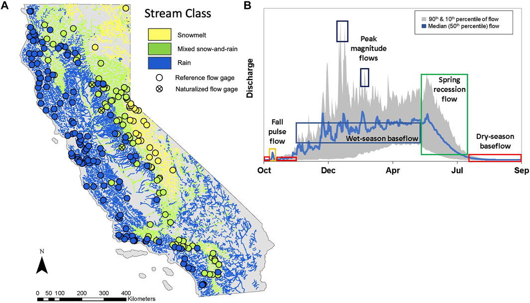
FIGURE 1. (A) Reference quality gages in California (n = 219) used for developing functional flow metric models, including 3 gages on large rivers with naturalized flow records (Supplementary Table S1). Gages and the stream network are shaded according to their hydrologic classification type (snowmelt-dominated, mixed snow-and-rain, and rainfall-dominated flow regimes), modified from Lane et al. (2017) and Patterson et al. (2020). (B) A representative hydrograph from a reference gage, highlighting five functional flow components for California streams, from Yarnell et al. (2020). Blue line represents median (50^th percentile) daily discharge. Gray shading represents 90–10^th percentiles of daily discharge over the period of record.

Streamflow Data and Functional Flow Metric Calculations

All gages operated by the U.S. Geological Survey (USGS) in California were screened to identify those considered to be reference-quality, following methods described by Zimmerman et al. (2018). Briefly, the watershed above each gage was evaluated using GIS-based methods and visual inspection of aerial imagery to exclude sites with evidence of significant human activities, including water diversions and storage reservoirs, intensive agriculture and forestry practices, dense road networks, and extensive impervious surfaces. We also reviewed USGS published annual data reports for each gage that note the influence of significant anthropogenic activities on observed flow records (Falcone et al., 2010). Through a subsequent manual screening process, several gages were removed from the analysis that exhibited irregular, impaired, and or aseasonal flow patterns. In total, we identified 216 reference gages in California, which included both active stations located on relatively pristine streams and gages with historical observations that pre-dated significant anthropogenic disturbances (e.g., prior to dam construction). We included an additional 3 gages located below dams for which reconstructed unimpaired flow data were available in order to increase the physiographic range represented in the dataset (California Department of Water Resources [DWR], 2007), bringing the total number of reference gages to 219 (Figure 1; Supplementary Table S1).

The resulting reference gage set includes periods of record as early as 1950 and as recent as 2015, with an average period of record of 33 years and ranging from 6 to 65 years (Supplementary Table S1). These gages are well distributed across the diversity of river types in California, including snowmelt (n = 25), rain (n = 125), and mixed snow-and-rain (n = 69) hydrologic regimes, following a simplified version of a stream classification scheme developed by Lane et al. (2017). The gages are located on streams with drainage areas ranging from 5 to 9,340 square kilometers and are distributed throughout California, with the exception of the arid southeastern corner of the state (Figure 1), where most streams are ephemeral and no reference gages are present. We confirmed that reference gages located in close proximity were separated by intervening tributaries or had distinct periods of record.

Complete years of daily flow data for all reference gages were downloaded from the USGS National Water Information System (USGS, 2017). Annual FFMs were then calculated from daily flow records using signal processing algorithms designed to characterize seasonal flow features of the annual hydrograph. The approach to calculate annual timing metrics detailed by Patterson et al. (2020) is as follows: A high standard deviation Gaussian filter was applied to daily streamflow time series to detect dominant peaks and valleys from the annual hydrograph. Localized search windows were set around hydrologic features of interest (e.g., annual peak flow). A low standard deviation Gaussian filter was then applied to the observed daily flow in the search window to identify seasonal shifts in the hydrograph, based on slope breaks in the derivative of a fitted spline curve. Break points were used to quantify the timing metrics for the wet season, dry season, and spring recession periods, from which seasonal magnitude, duration, frequency, and rate of change metrics could then be calculated. The spring recession rate was calculated as the median daily rate of change in flow from the start date of the spring recession until the start of the dry season, considering only days with negative change to omit storm events during the recession period. Peak flow magnitudes were calculated as the long-term annual flood exceedance flow associated with the 2-, 5-, and 10-years recurrence intervals. We also calculated peak flow duration (cumulative number of days in which this peak flow magnitude is exceeded) and frequency (number of times the flow magnitude is exceeded), in each of the years in which a flood of a given recurrence interval occurred. Following these methods, we calculated the values of 24 FFMs, describing 5 functional flow components, at each reference gage (Table 1; Figure 1).

TABLE 1

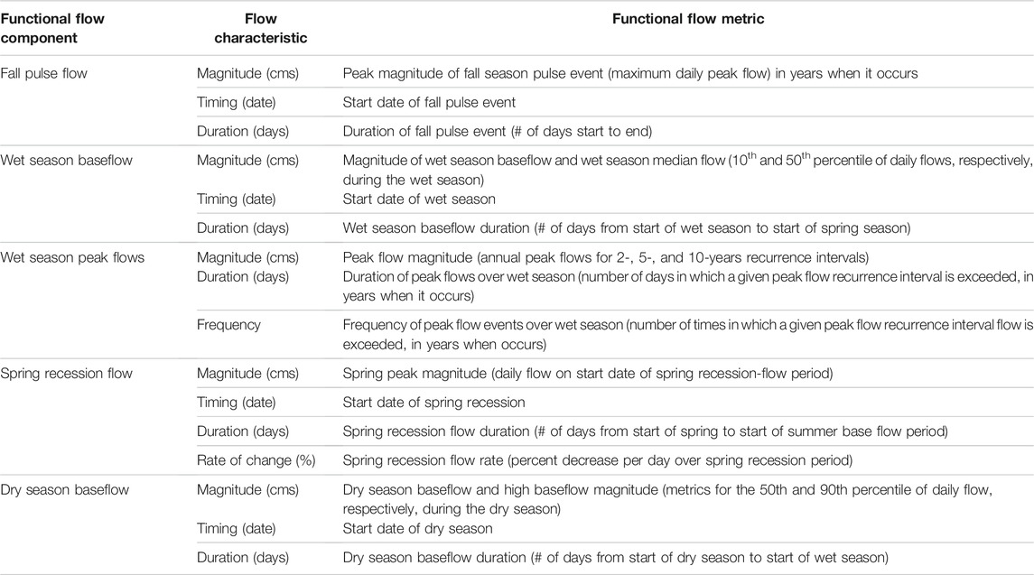
TABLE 1. Functional flow metrics for which machine learning models were developed and their corresponding functional flow components and characteristics. There are a total of 24 metrics that represent five functional flow components. Note that there are 2 metrics describing the magnitudes of wet season baseflow and dry season baseflow and 3 metrics describing each of the peak flow characteristics (2-, 5-, and 10-years recurrence interval floods) in the wet season.

Next, we used a GIS-based approach to calculate over 150 variables related to physical attributes of the watershed above each reference gage using publicly available geospatial datasets (Supplementary Table S1). These included variables related to topography (e.g., elevation, slope, and aspect, etc.), dominant geology and soil types (e.g., granitic, volcanic, or sedimentary, and mean content of clay, sand, and silt, etc.), and watershed hydraulic properties (e.g., topographic wetness index, baseflow index, mean depth to water table, etc.). We also included time-varying climatic variables including mean monthly temperature and precipitation from the 800-m PRISM dataset from Daly et al. (2008), as well as expected monthly runoff from McCabe and Wolock (2011). These climate variables were expressed as monthly, seasonal, and annual values for each year of FFM observations at a reference site, as well as for years preceding the FFM observations (Supplementary Table S2).

Functional Flow Metric Modeling

Random forest (RF) models (Cutler et al., 2012) were developed for each FFM. For most FFMs, observed values were calculated for each year of the reference period of each gage. For peak flow magnitude FFMs, single values for the 2-, 5-, and 10-years recurrence interval flood were estimated at each gage. Each RF model specified a FFM as the response variable and a total of 182 watershed and climate variables as predictor variables (Supplementary Table S2; Carlisle, 2022). All models were run using 2000 trees and default parameters with the randomForest function in the randomForest package, version 4.6 (Liaw and Wiener, 2018) in R (R Core Team, 2020).

Random forest models include a resampling routine that provides estimates of model performance comparable to what is obtained from independent validation data. However, because our dataset included repeated observations of FFM values from each of the 219 reference sites, the replicate datasets generated from RF’s internal sampling could produce overly optimistic estimates of model performance. We therefore used a leave-one-out cross-validation approach to estimate model performance, in which each reference site (including observations for all years of record) was excluded in turn from a calibration dataset, following methods by Eng et al. (2017); Zimmerman et al. (2018). The trained model was subsequently used to predict FFM values at the excluded reference site. We retained the 10th, 25th, 50th, 75th, and 90th percentiles of the predictions generated by the 2000 trees for each excluded reference site. For each model iteration, we also identified the most influential predictor variables, based on their Gini index (Cutler et al., 2007), which measures the loss of model predictive accuracy when that variable is excluded. Higher values indicate greater importance in contributing to the accuracy of the models.

To assess model performance, we compared predicted FFM values with observations at sites excluded from model training. We restricted the assessment to sites with 20 or more observations (i.e., 20 years of record) and calculated several model performance criteria to limit the risk of flawed interpretation resulting from the use of a single performance metric (Clark et al., 2021). We calculated performance criteria that provided measures of both the dispersion and central tendency of model predictions in comparison to observed values. First, we compared the distribution of observed to predicted values of FFMs by calculating the percent of annual observed values at a site that fell within the predicted interquartile range (IQR, range between the 25th to 75th percentile values) and the inter-80th percentile range (I80R, range between the 10th to 90th percentile values) for that site. The mean of these percentage values across all sites was used to assess the overall degree to which the distribution of observations aligned with the predicted range of each metric. Models with perfect performance would have percentage values of 50% for the IQR criterion and 80% for the I80R criterion, indicating that, on average, 50% and 80% of the observed values fall within the predicted IQR and I80R, respectively. Models that under-estimate the natural range of variation in FFMs would have values below 50% and 80%, respectively, and models that over-estimate the range of variation would exceed these values.

To evaluate accuracy for the central tendency of model predictions, we also compared the median value of observations to the median value of predictions at each site. The paired values were used to calculate several “goodness-of-fit” criteria commonly used in hydrologic model performance assessment (Moriasi et al., 2007; Eng et al., 2017): the observed-to-expected ratio (O/E), the coefficient of determination (r²), percent bias, and Nash-Sutcliffe Efficiency (NSE). We then calculated the mean value of each performance criterion across all sites. For the peak flow magnitude metrics, we only calculated the performance measures of central tendency because only single values were available for each site (i.e., 2-, 5-, and 10-years recurrence interval peak flows). Due to the skewed distribution of peak flow frequency and duration metrics to low values, measures of central tendency were unreliable. For those metrics, we excluded observations with zero values and considered only the distribution of observations relative to the predicted range of values, by calculating the percentage of observations falling within the predicted IQR and I80R, as described above.

To evaluate model performance across all criteria, we standardized the values of all calculated criteria between 0 (poor performance) and 1 (perfect performance). To scale O/E values, we retained values less than 1 and calculated the inverse of those greater than 1. To scale percent bias, we subtracted values from 100 and then divided by 100. NSE values less than 0 were set to 0 and no changes were made to the r² values. To scale the IQR criterion, the absolute value of difference between the calculated value and 50 was divided by 50 and subtracted from 1. Similarly for I80R, the absolute value of difference between the calculated value and 80 was divided by 80 and subtracted from 1. We then developed a composite performance index by averaging the values of all six criteria. We assigned a qualitative performance rating to the composite performance index values excellent (>0.9), very good (0.81–0.9), good (0.65–0.8), satisfactory (0.5–0.64), and poor (<0.5) model performance, following guidelines similar to Moriasi et al. (2007).

Finally, we evaluated spatial bias in model performance by separating reference gages into stream classes (Lane et al., 2017). We grouped gages into one of three classes based on their dominant hydrologic characteristics: snowmelt, rain, and mixed snow-and-rain. We then compared model predictions and observed data from reference gages occurring within each stream class, using the same set of performance criteria, and again calculated the composite performance index for each metric.

Predicting Functional Flows Across the Stream Network

After the model performance evaluation, we used the RF models to predict the natural range of functional flows for all stream reaches in California. We trained final models (n = 2000 trees) with the full set of reference gages to include the maximum amount of information possible. We then calculated the same set of watershed and climate variables used in model training, obtained from Wieczorek et al. (2018), for 142,509 natural stream reaches (mean length = 2.1 km; sd length = 2.0 km) represented by the National Hydrography Dataset for California (NHDPlus, Version2) (Horizon Systems Corporation, 2012). These data were used to predict FFM values from 1950 to 2015 at each stream reach from the trained RF models. The 10th, 50th, and 90th percentiles of model predictions for each FFM were calculated for each stream reach. Predicted ranges were compiled for all years (1950–2015) and for all dry, moderate, and wet water years and made available on a public website (California Environmental Flows Working Group [CWFWG], 2021). Reported values represent the expected natural range of FFMs at each stream, also accounting for model prediction uncertainty.

Results

Variable Influences on Functional Flow Metrics

Climate variables were generally the most influential predictors in the FFM models, although physical catchment variables were important for some metrics (Table 2; Supplementary Table S3). For the fall pulse metrics, climate variables including precipitation, temperature, and runoff for fall season months (e.g., Oct, Nov) were consistently among the most influential variables. The rainfall-runoff erosivity index, which reflects the estimated amount and rate of runoff produced by a storm (Renard et al., 1997), was also influential in predicting fall pulse flow duration. Wet season baseflow metrics were strongly influenced by monthly climate variables corresponding to winter months (e.g., December runoff) and multi-annual antecedent precipitation, runoff, and temperature variables were generally the most important variables in the models. Precipitation and runoff had a stronger influence on wet season baseflow magnitudes and duration, whereas temperature had a stronger influence on wet season baseflow timing.

TABLE 2

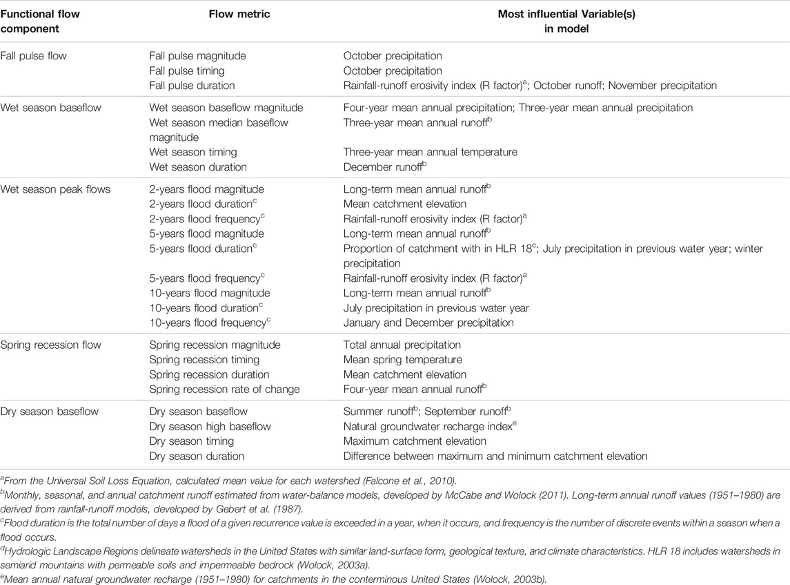
TABLE 2. Most influential variables for each functional flow metric model, as determined by the Gini index. Only the most influential variable is reported, unless the next most influential variable was within the 10% of its Gini index value. See Supplementary Table S2 for predictor variable descriptions and Supplementary Table S3 for the Gini index values for all variables in each model.

Peak flow magnitudes, including 2-, 5-, and 10-years recurrence interval peak flow metrics, were most influenced by the catchment’s long-term mean annual runoff (Gebert et al., 1987) as well as mean maximum and mean annual precipitation (Table 2; Supplementary Table S3). Peak flow duration–the number of days in a year in which flows exceeded a peak flow threshold–was most influenced by monthly precipitation variables in the winter months and the previous water year, catchment mean elevation, and the hydrologic landscape region in which the catchment predominately occurs (Wolock, 2003a). Peak flow frequency—the number of peak flow events in a year of a given recurrence interval—was also most influenced by precipitation in winter months and antecedent year, as well as the catchment’s rainfall-runoff erosivity index and groundwater recharge index (Wolock, 2003b).

Annual precipitation and runoff had the greatest influence on spring recession magnitude, whereas mean temperatures in the spring months and spring season had the greatest influence on spring recession timing (Table 2; Supplementary Table S3). The duration of the spring recession flow period was most influenced by catchment elevation, the clay content of catchment soils, winter precipitation, and monthly runoff in December and June, near the start, and end of the wet season, respectively and the rate-of-change by mean runoff observed over the most recent four-year period. Spring rate-of-change was most influenced by runoff variables, including annual runoff for the water year and multi-annual antecedent periods.

Runoff variables were also influential in predicting dry season baseflow characteristics. Runoff in the summer months and seasonally-averaged runoff were both important in predicting dry season baseflow magnitudes. The catchment groundwater recharge index was also influential for the dry season high baseflow metric. Catchment variables were most important in predicting the timing of the dry season. Influential variables included the mean and max catchment elevation, the baseflow index, and soil properties (Supplementary Table S3). Similar to the fall and spring duration metrics, duration of the dry season was most influenced by catchment properties, including elevation, spring precipitation, and the catchment erodibility index (K-factor).

Model Performance

Overall, the FFM models had high predictive accuracy, with all 24 metrics exhibiting excellent (composite performance index [CPI] > 0.9 for 7 metrics), very good (0.8 < CPI ≤0.9 for 12 metrics) or good (0.65 < CPI ≤0.8 for 5 metrics) performance (Figure 2; Supplementary Table S4). The models performed well in predicting fall pulse flows, including the magnitude (CPI = 0.85), timing (CPI = 0.80), and duration (CPI = 0.70). The slightly lower CPI for fall pulse duration was driven by low NSE and r² performance criteria values (<0.25). This was the result of the limited range of whole number values in the observation record (median fall pulse duration of 2–7 days among all sites), such that slight deviation of predictions (i.e., 1 or 2 days) caused NSE and r² values to substantially decrease.

FIGURE 2

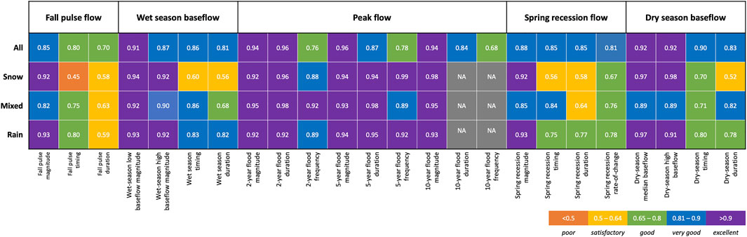
FIGURE 2. Model performance summary for functional flow components and metrics for all streams and for streams stratified by stream type (mixed snow-and-rain, rainfall-dominant, and snowmelt-dominant). The composite performance index values shown are calculated as the mean of multiple, standardized performance criteria values (Supplementary Tables S4, S5).

The models for wet season baseflow accurately predicted all metrics, especially the wet season low magnitude metric (CPI = 0.91), and exhibited excellent performance (CPI >0.9) in predicting peak flow magnitudes for 2-, 5-, and 10-years flood recurrence intervals. Model performance for within-year flood frequency and duration were also considered good, very good, or excellent. The model for the 10-years flood frequency tended to overestimate the observed range of variation (i.e., a higher proportion of observed values fell within the predicted interquartile range than expected; Supplementary Table S4), although overall model performance was still good. Model performance was very good (CPI >0.8) for spring recession flow magnitude, timing, duration, and rate-of-change. The models were very good or excellent in predicting all dry season baseflow metrics, including the median (CPI = 0.92) and high baseflow magnitudes (CPI = 0.92), dry season timing (CPI = 0.90), and dry season duration (CPI = 0.83).

When model performance was assessed by stream class, the CPI deviated from those obtained when all streams were evaluated together (Figure 2). For snowmelt-dominated streams, the models performed less well in predicting timing and duration metrics, including for the fall pulse, wet season, spring recession, and dry season. However, only the fall pulse timing model was considered “poor” performing for the snowmelt stream class. Model performance declined for some metrics in the mixed snow-and-rain and rainfall-dominated classes, but all models were considered at least satisfactory and most were very good or excellent (Figure 2). Stream gage records were insufficient to evaluate the performance of the 10-years flood duration and frequency metrics by stream class.

Model Predictions

Based on the overall satisfactory performance of the FFM models, predictions of expected, natural FFM values were generated for all stream reaches in California using models calibrated with the full set of reference gages. Model predictions were compiled in a geospatial database and made available through an online mapping tool to allow users to visualize and download estimates of natural FFM values for any stream reach in the state CEFWG, 2021 (Figure 3).

FIGURE 3

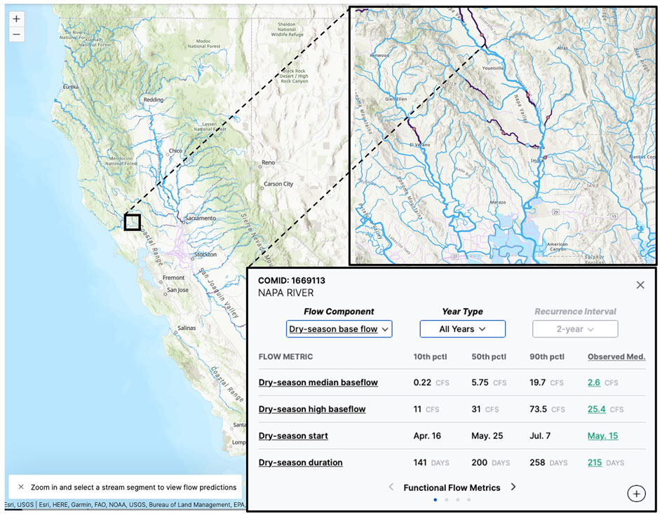
FIGURE 3. Screenshot of online mapping tool developed to explore, visualize, and download modeled natural functional flow metrics for streams in California, displaying dry season baseflow metrics at a gaged stream reach of the Napa River. Available at: https://rivers.codefornature.org.

Discussion

Here we applied a machine learning modeling approach to estimate functional flows for over 140,000 stream reaches exceeding 250,000 km in total length in California, United States. Our evaluation of model performance indicated that natural hydrologic signatures describing the magnitude, timing, duration, frequency, and rate-of-change of functional components of the flow regime could be accurately predicted across a large region with high geographic variability. For every stream reach in the state, we generated predictions for the expected natural range of five functional flow components, including fall pulse flows, wet season baseflows, peak flows, spring recession flows, and dry season baseflows. By predicting the range of flows that are expected to support essential ecosystem functions under natural landscape conditions, these estimates can serve as a foundation for assessing ecological flow needs, quantifying flow alteration, and guiding development of environmental flow recommendations in the state, through the California Environmental Flows Framework (Stein et al., 2021) or other environmental flow assessment approaches.

The models relied on a network of reference-quality gages and a broad suite of watershed variables to predict functional flow metrics. For most metrics, these variables appeared to capture the effects of dominant physical processes that control seasonal flow dynamics. In particular, the models were highly accurate in predicting the magnitudes of fall pulse and wet season peak flows, as well as wet and dry season baseflows. In contrast, the models did not perform as well in predicting the timing and duration of flow components. This likely relates to the monthly scale of the climate predictor variables, which fail to represent physical processes that control the timing and duration of functional flow components at shorter timescales. These deficiencies were more pronounced when evaluating model performance by stream class. For example, model performance was substantially lower for timing and duration metrics in the snow-dominated stream class, which might relate to the inability of the model to capture snow accumulation and snowmelt runoff dynamics. Nevertheless, model performance remained satisfactory or better for all but one metric: fall pulse timing in the snow class.

The modeling approach used in this study differs from physically-based hydrologic models (i.e., rainfall-runoff models) that are commonly used in environmental flow applications. First, rainfall-runoff models are generally trained and calibrated using a small sample of streamflow gaging records to estimate streamflow throughout individual watersheds based on intensive field data collection and parameterization. In contrast, the modeling approach used here relies on a large network of gages and can be applied to generate predictions across a broad geographic region. Model calibration procedures also differ. Rainfall-runoff models are often run on daily or sub-daily timescales and are calibrated to generate the best fit with observed streamflow data. This means that model parameters are generally tuned to minimize deviation in all elements of the flow regime and, as a result, there may be tradeoffs associated with improving predictive accuracy in some flow components (e.g., peak flows) at the expense of others (e.g., low flows). In contrast, the modeling approach described here calibrates to specific aspects of the flow regime, avoiding such tradeoffs, and likely increasing model predictive accuracy of functional flow metrics.

Hydrologic models are typically evaluated using a limited set of “goodness of fit” (GOF) criteria, such as r-squared and NSE, to compare predictions with paired observations (Clark et al., 2021). The performance assessment approach used in this study used a broader suite of criteria, including both GOF and measures that evaluate the degree to which the distributions of predictions align with observations. We found there was notable variation in the performance criteria values for several metrics (Supplementary Tables S4, S5). This indicates that interpretation of model accuracy can be highly influenced by the selection of performance criteria and suggests that multiple criteria should be used to assess hydrologic model performance where possible.

One of the shortcomings of statistical models is that they do not explicitly represent the mechanisms that control streamflow generation and variability. Although the variable importance rankings can provide some insight into the physical controls on specific flow components, factors contributing to model accuracy can be difficult to ascertain. For example, the relationship between seasonal precipitation (and runoff) volumes and the magnitudes of functional flow components was evident in the variable important plots of the RF models. In the dry season, the importance of the groundwater recharge index (Wolock, 2003b) suggested that this variable was, at least in part, effective in representing groundwater-surface interactions that influence baseflow. The strong influence of spring temperature on the timing of the spring flow recession was also consistent with understanding of the physical controls on spring snowmelt dynamics (Yarnell et al., 2010). However, the influences of other variables on functional flow metrics were more difficult to interpret. For example, catchment elevation was important in predicting the duration of the 2-years flood, spring recession duration, and dry season duration, but the physical basis for these relationships is less clear. Additional studies that offer robust comparisons between statistical and physically-based models, such as performed by Hodgkins et al. (2020), would be helpful for evaluating the benefits and limitations of different hydrologic modeling approaches in predicting functional flows and supporting environmental flow applications.

One important limitation in our modeling approach is the network of available reference gages. The USGS stream gaging network is biased towards larger, perennial streams of management interest (Kiang et al., 2013), and these biases are also evident in our study area. In particular, there is poor representation of intermittent and ephemeral streams among reference gages (Hammond et al., 2021), especially in the arid southeastern region of California. Similarly, spring-fed streams and those highly dependent on groundwater interactions are poorly represented in the reference gage network. In addition, most large streams and rivers in the state have been altered by dams, diversions, and land use change, among other human activities (Zimmerman et al., 2018), so there are few locations that are considered reference-quality in these larger rivers. We addressed this limitation, in part, by including reconstructed natural flow records from a few major rivers below dams (DWR, 2007). However, we recognize that predictions of FFMs are likely less reliable in these and other poorly gaged systems compared to better-gaged portions of the stream network. Unfortunately, the degree to which model performance is affected by gage network gaps is difficult to quantify because the absence of gages for model training also means there are no gages for model validation. Strategically installing new gages in reference-quality streams that represent these unique hydrologic contexts would help improve the accuracy, aid quantification of uncertainty, and enhance the utility of the models in environmental flow management applications across a broader range of stream types. Limiting human catchment disturbance would also help ensure streams remain as reference-quality in the future.

In addition to obtaining data from a wider representation of reference-quality streams, the performance of functional flow models could be improved with new geospatial data that describe hydrologically relevant watershed characteristics. In particular, improved characterization of watershed lithology, which has a strong effect on subsurface flow dynamics, is likely to be helpful in predicting flow recession patterns and baseflow conditions (Lovill et al., 2018). Advancements in satellite sensing products for assessing vegetation dynamics, surface water, and groundwater levels (Tang et al., 2009) also hold enormous potential for improving the characterization of watersheds and enhancing model performance. We acknowledge that more work is needed to understand how changing climatic conditions will influence flow regimes and supported functions (Grantham et al., 2018). The current modeling approach estimates the range of variation in functional flow metrics based on historical (1950–2015) climate, watershed conditions, and flow responses. As California and the world experience novel climate conditions, retraining models with contemporary data will be necessary to generate new predictions for the flow regime and to evaluate whether critical ecosystem functions will continue to be supported as flow components shift in response to climate change.

Conclusion

The modeling approach presented here can be used to develop an initial estimate of flows required to sustain essential ecological functions and establish a foundation upon which subsequent analyses can be performed. These modeled natural functional flow predictions provide a reference condition against which to evaluate potential alterations to critical ecosystem functions due to human management activities or climate changes. For systems with specific management objectives or where ecosystems have been highly altered, more intensive studies will likely be needed to determine if the functional flows estimated by the models are appropriate for quantifying ecological flow needs (e.g.,Taniguchi-Quan et al., 2022). In addition, support and guidance for adaptively managing environmental flows to maximize their effectiveness will help sustain ecosystem functions and health, particularly in a changing climate (John et al., 2020). Efforts to integrate the functional flows modeling approach in an environmental flow program in California are promising (Stein et al., 2021). As a relatively simple and cost-effective means for supporting regional environmental flow programs, there is also potential to adapt the approach for use in other geographic contexts, including data-poor regions of the world. Together with other advances in environmental flow science, functional flows models could play an important role in accelerating much-needed protections of environmental flows at a global scale.

Data Availability Statement

The datasets presented in this study can be found in online repositories, which are cited in this article or provided as supplementary material. Questions regarding the data and code used in the analysis can be directed to the corresponding author.

Author Contributions

TG led the preparation of this manuscript. TG, DC, JZ, BL, and KT-Q contributed to model development and evaluation. TG, JH, BL, RL, AO, SS-S, BS, ES, SY, JZ, and KT-Q contributed to the development of the California Environmental Flows Framework, theoretical concepts guiding the modeling approach, and to writing, review, and editing of this manuscript.

Funding

Funding for this work was provided by the California State Water Resources Control Board (Agreement #16-062-300) and The Nature Conservancy. Open access publication fees were provided by the University of California, Berkeley Library.

Conflict of Interest

The authors declare that the research was conducted in the absence of any commercial or financial relationships that could be construed as a potential conflict of interest.

Publisher’s Note

All claims expressed in this article are solely those of the authors and do not necessarily represent those of their affiliated organizations, or those of the publisher, the editors and the reviewers. Any product that may be evaluated in this article, or claim that may be made by its manufacturer, is not guaranteed or endorsed by the publisher.

Acknowledgments

Any use of trade, firm, or product names is for descriptive purposes only and does not imply endorsement by the U.S. Government. We would like to thank members of the Environmental Flows Working Group of the California Water Quality Monitoring Council for valuable feedback on the California Environmental Flows Framework and the modeling approach presented here. This paper was written in Berkeley, California, which sits on the homelands of the xučyun (Huichin), the ancestral and unceded land of the Chochenyo speaking Ohlone people.

Supplementary Material

The Supplementary Material for this article can be found online at: https://www.frontiersin.org/articles/10.3389/fenvs.2022.787473/full#supplementary-material

References

Arthington, A. H., Bhaduri, A., Bunn, S. E., Jackson, S. E., Tharme, R. E., Tickner, D., et al. (2018). The Brisbane Declaration and Global Action Agenda on Environmental Flows (2018). Front. Environ. Sci. 6, 45. doi:10.3389/fenvs.2018.00045

CrossRef Full Text | Google Scholar

California Department of Water Resources [DWR], Bay-Delta Office (2007). California Central Valley Unimpaired Flow Data. Fourth Edition. Sacramento, CA: California Department of Water Resources. Available at: https://www.waterboards.ca.gov/waterrights/water_issues/programs/bay_delta/bay_delta_plan/water_quality_control_planning/docs/sjrf_spprtinfo/dwr_2007a.pdf [Accessed January 15, 2022].

Google Scholar

California Environmental Flows Working Group [CWFWG] (2021). California Natural Flows Database: Functional Flow Metrics, v1.2.1. Available at: https://rivers.codefornature.org/ [Accessed January 15, 2022].

Google Scholar

Carlisle, D. M. (2022). Functional Flow Metrics Data Release for Select Reference Sites in California: Data Release for Functional Flow Modeling. USGS Data Release. Reston, Virginia: U.S. Geological Survey. doi:10.5066/P9PF101N

CrossRef Full Text | Google Scholar

Clark, M. P., Vogel, R. M., Lamontagne, J. R., Mizukami, N., Knoben, W., Tang, G., et al. (2021). The Abuse of Popular Performance Metrics in Hydrologic Modeling. Water Resour. Res. 57, e2020WR029001. doi:10.1029/2020wr029001

CrossRef Full Text | Google Scholar

Cutler, A., Cutler, D. R., and Stevens, J. R. (2012). “Random Forests,” in Ensemble Machine Learning: Methods And Applications. Editors C. Zhang, and Y. Ma (Boston, MA: Springer US), 157–175. doi:10.1007/978-1-4419-9326-7_5

CrossRef Full Text | Google Scholar

Cutler, D. R., Edwards, T. C., Beard, K. H., Cutler, A., Hess, K. T., Gibson, J., et al. (2007). Random Forests for Classification in Ecology. Ecology 88, 2783–2792. doi:10.1890/07-0539.1

PubMed Abstract | CrossRef Full Text | Google Scholar

Daly, C., Halbleib, M., Smith, J. I., Gibson, W. P., Doggett, M. K., Taylor, G. H., et al. (2008). Physiographically Sensitive Mapping of Climatological Temperature and Precipitation across the Conterminous United States. Int. J. Climatol. 28, 2031–2064. doi:10.1002/joc.1688

CrossRef Full Text | Google Scholar

Eng, K., Grantham, T. E., Carlisle, D. M., and Wolock, D. M. (2017). Predictability and Selection of Hydrologic Metrics in Riverine Ecohydrology. Freshw. Sci. 36, 915–926. doi:10.1086/694912

CrossRef Full Text | Google Scholar

Escobar-Arias, M. I., and Pasternack, G. B. (2010). A Hydrogeomorphic Dynamics Approach to Assess In-Stream Ecological Functionality Using the Functional Flows Model, Part 1-model Characteristics. River Res. Applic. 26, 1103–1128. doi:10.1002/rra.1316

CrossRef Full Text | Google Scholar

Falcone, J. A., Carlisle, D. M., Wolock, D. M., and Meador, M. R. (2010). GAGES: A Stream Gage Database for Evaluating Natural and Altered Flow Conditions in the Conterminous United States. Ecology 91, 621. doi:10.1890/09-0889.1

CrossRef Full Text | Google Scholar

Gebert, W. A., Graczyk, D. J., and Krug, W. R. (1987). Average Annual Runoff in the United States, 1951-80. U.S. Geological Survey Report, 710. doi:10.3133/ha710

CrossRef Full Text | Google Scholar

Gillilan, D. M., and Brown, T. C. (1997). Instream Flow Protection: Seeking A Balance in Western Water Use. Washington, D.C.: Island Press.

Google Scholar

Grantham, T. E., Mount, J., Stein, E. D., and Yarnell, S. M. (2020). Making the Most of Water for the Environment: A Functional Flows Approach for California’s Rivers. San Francisco, CA: Public Policy Institute of California Water Policy Center. Available at: https://www.ppic.org/publication/making-the-most-of-water-for-the-environment/ [Accessed January 15, 2022].

Google Scholar

Grantham, T. E. W., Carlisle, D. M., McCabe, G. J., and Howard, J. K. (2018). Sensitivity of Streamflow to Climate Change in California. Climatic Change 149, 427–441. doi:10.1007/s10584-018-2244-9

CrossRef Full Text | Google Scholar

Grill, G., Lehner, B., Thieme, M., Geenen, B., Tickner, D., Antonelli, F., et al. (2019). Mapping the World's Free-Flowing Rivers. Nature 569, 215–221. doi:10.1038/s41586-019-1111-9

PubMed Abstract | CrossRef Full Text | Google Scholar

Hammond, J. C., Zimmer, M., Shanafield, M., Kaiser, K., Godsey, S. E., Mims, M. C., et al. (2021). Spatial Patterns and Drivers of Nonperennial Flow Regimes in the Contiguous United States. Geophys. Res. Lett. 48, e2020GL090794. doi:10.1029/2020gl090794

CrossRef Full Text | Google Scholar

Hodgkins, G. A., Dudley, R. W., Russell, A. M., and LaFontaine, J. H. (2020). Comparing Trends in Modeled and Observed Streamflows at Minimally Altered Basins in the United States. Water 12, 1728. doi:10.3390/w12061728

CrossRef Full Text | Google Scholar

Horizon Systems Corporation (2012). NHDPlus Version 2. Available at: https://nhdplus.com/NHDPlus/NHDPlusV2_home.php [Accessed January 15, 2022].

Google Scholar

Horne, A., Webb, A., Stewardson, M., Richter, B., and Acreman, M. (2017). Water for the Environment: From Policy and Science to Implementation and Management. London: Academic Press.

Google Scholar

John, A., Nathan, R., Horne, A., Stewardson, M., and Webb, J. A. (2020). How to Incorporate Climate Change into Modelling Environmental Water Outcomes: a Review. J. Water Clim. Chang. 11, 327–340. doi:10.2166/wcc.2020.263

CrossRef Full Text | Google Scholar

Kiang, J. E., Stewart, D. W., Archfield, S. A., Osborne, E. B., and Eng, K. (2013). A National Streamflow Network gap Analysis. Scientific Investigations Report 2013-5013. doi:10.3133/sir20135013

CrossRef Full Text | Google Scholar

Lane, B. A., Dahlke, H. E., Pasternack, G. B., and Sandoval‐Solis, S. (2017). Revealing the Diversity of Natural Hydrologic Regimes in California with Relevance for Environmental Flows Applications. J. Am. Water Resour. Assoc. 53, 411–430. doi:10.1111/1752-1688.12504

CrossRef Full Text | Google Scholar

Liaw, A., and Wiener, M. (2018). Package “randomForest”: Breiman and Cutler’s Random Forests for Classification and Regression. Available at: https://cran.r-project.org/web/packages/randomForest/randomForest.pdf [Accessed January 15, 2022].

Google Scholar

Lovill, S. M., Hahm, W. J., and Dietrich, W. E. (2018). Drainage from the Critical Zone: Lithologic Controls on the Persistence and Spatial Extent of Wetted Channels during the Summer Dry Season. Water Resour. Res. 54, 5702–5726. doi:10.1029/2017wr021903

CrossRef Full Text | Google Scholar

McCabe, G. J., and Wolock, D. M. (2011). Independent Effects of Temperature and Precipitation on Modeled Runoff in the Conterminous United States. Water Resour. Res. 47, W11522. doi:10.1029/2011wr010630

CrossRef Full Text | Google Scholar

Moriasi, D. N., Arnold, J. G., Van Liew, M. W., Bingner, R. L., Harmel, R. D., and Veith, T. L. (2007). Model Evaluation Guidelines for Systematic Quantification of Accuracy in Watershed Simulations. Trans. ASABE 50, 885–900. doi:10.13031/2013.23153

CrossRef Full Text | Google Scholar

Obester, A. N., Lusardi, R. A., Santos, N. R., Peek, R. A., and Yarnell, S. M. (2022). The Use of Umbrella Fish Species to Provide a More Comprehensive Approach for Freshwater Conservation Management. Aquat. Conserv. 32, 112–128. doi:10.1002/aqc.3746

CrossRef Full Text | Google Scholar

Patterson, N. K., Lane, B. A., Sandoval-Solis, S., Pasternack, G. B., Yarnell, S. M., and Qiu, Y. (2020). A Hydrologic Feature Detection Algorithm to Quantify Seasonal Components of Flow Regimes. J. Hydrol. 585, 124787. doi:10.1016/j.jhydrol.2020.124787

CrossRef Full Text | Google Scholar

Poff, N. L., Allan, J. D., Bain, M. B., Karr, J. R., Prestegaard, K. L., Richter, B. D., et al. (1997). The Natural Flow Regime. Bioscience 47, 769–784. doi:10.2307/1313099

CrossRef Full Text | Google Scholar

Poff, N. L., Richter, B. D., Arthington, A. H., Bunn, S. E., Naiman, R. J., Kendy, E., et al. (2010). The Ecological Limits of Hydrologic Alteration (ELOHA): a New Framework for Developing Regional Environmental Flow Standards. Freshw. Biol. 55, 147–170. doi:10.1111/j.1365-2427.2009.02204.x

CrossRef Full Text | Google Scholar

R Core Team (2020). R: A Language and Environment for Statistical Computing. Vienna, Australia: R Foundation for Statistical Computing. Available at: https://www.R-project.org [Accessed October 15, 2020].

Google Scholar

Reid, A. J., Carlson, A. K., Creed, I. F., Eliason, E. J., Gell, P. A., Johnson, P. T. J., et al. (2019). Emerging Threats and Persistent Conservation Challenges for Freshwater Biodiversity. Biol. Rev. 94, 849–873. doi:10.1111/brv.12480

PubMed Abstract | CrossRef Full Text | Google Scholar

Renard, K. G., Foster, C. R., Weesies, G. A., McCool, D. K., and Yoder, D. C. (1997). “Predicting Soil Erosion by Water: A Guide to Conservation Planning with the Revised Universal Soil Loss Equation (RUSLE),” in US Department of Agriculture, Agriculture Handbook Number 703 (Washington, DC: Government Printing Office), 47–51.

Google Scholar

Stein, E. D., Zimmerman, J., Yarnell, S., Stanford, B., Lane, B., Taniguchi-Quan, K., et al. (2021). The California Environmental Flows Framework: Meeting the challenge of Developing a Large-Scale Environmental Flows Program. Front. Environ. Sci. 9, 769943. doi:10.3389/fenvs.2021.769943

CrossRef Full Text | Google Scholar

Tang, Q., Gao, H., Lu, H., and Lettenmaier, D. P. (2009). Remote Sensing: Hydrology. Prog. Phys. Geogr. Earth Environ. 33, 490–509. doi:10.1177/0309133309346650

CrossRef Full Text | Google Scholar

Taniguchi-Quan, K. T., Irving, K., Stein, E. D., Poresky, A., Wildman, R., Aprahamian, A., et al. (2022). Developing Ecological Flow Needs in a Highly Altered Region: Application of California Environmental Flows Framework in Southern California, USA. Front. Environ. Sci. 10, 787631. doi:10.3389/fenvs.2022.787631

CrossRef Full Text | Google Scholar

Tickner, D., Opperman, J. J., Abell, R., Acreman, M., Arthington, A. H., Bunn, S. E., et al. (2020). Bending the Curve of Global Freshwater Biodiversity Loss: An Emergency Recovery Plan. Bioscience 70, 330–342. doi:10.1093/biosci/biaa002

PubMed Abstract | CrossRef Full Text | Google Scholar

U.S. Geological Survey (2017). USGS water data for the Nation: U.S. Geological Survey National Water Information System database. [Accessed January 15, 2022]. doi:10.5066/F7765D7V

CrossRef Full Text | Google Scholar

Wieczorek, M. E., Jackson, S. E., and Schwarz, G. E. (2018). Select Attributes for NHDPlus Version 2.1 Reach Catchments and Modified Network Routed Upstream Watersheds for the Conterminous United States (Ver. 3.0, January 2021). U.S. Geological Survey data release. Reston, Virginia: U.S. Geological Survey. doi:10.5066/F7765D7V

CrossRef Full Text | Google Scholar

Wolock, D. M. (2003b). Estimated Mean Annual Natural Ground-Water Recharge in the Conterminous United States. US Geological Survey. Open File Report No. 2003-311. doi:10.3133/ofr03311

CrossRef Full Text | Google Scholar

Wolock, D. M. (2003a). Hydrologic Landscape Regions of the United States. US Geological Survey. Open-File Report No. 2003-145. doi:10.3133/ofr03145

CrossRef Full Text | Google Scholar

Yarnell, S. M., Petts, G. E., Schmidt, J. C., Whipple, A. A., Beller, E. E., Dahm, C. N., et al. (2015). Functional Flows in Modified Riverscapes: Hydrographs, Habitats and Opportunities. Bioscience 65, 963–972. doi:10.1093/biosci/biv102

CrossRef Full Text | Google Scholar

Yarnell, S. M., Stein, E. D., Webb, J. A., Grantham, T., Lusardi, R. A., Zimmerman, J., et al. (2020). A Functional Flows Approach to Selecting Ecologically Relevant Flow Metrics for Environmental Flow Applications. River Res. Applic 36, 318–324. doi:10.1002/rra.3575

CrossRef Full Text | Google Scholar

Yarnell, S. M., Viers, J. H., and Mount, J. F. (2010). Ecology and Management of the spring Snowmelt Recession. Bioscience 60, 114–127. doi:10.1525/bio.2010.60.2.6

CrossRef Full Text | Google Scholar

Zimmerman, J. K. H., Carlisle, D. M., May, J. T., Klausmeyer, K. R., Grantham, T. E., Brown, L. R., et al. (2018). Patterns and Magnitude of Flow Alteration in California, USA. Freshw. Biol. 63, 859–873. doi:10.1111/fwb.13058

CrossRef Full Text | Google Scholar