Time-Lapse Electrical Resistivity Tomography Imaging of Buried Human Remains in Simulated Mass and Individual Graves

Introduction

Law enforcement experts and forensic scientists are often engaged in searching for clandestine graves and locating buried human remains in homicide cases to bring justice to the victims and closure for families (Pringle et al., 2021). Victims are typically hidden by criminals in hurriedly excavated shallow individual graves with dimensions of 1 m × 0.5 m and less than 1 m deep (Pringle et al., 2008). On a larger scale, forensic search and recovery are also embarked upon to locate, recover, and identify victims of natural and man-made disasters, including earthquakes, tsunamis, and genocides (Varlet et al., 2020). Hence, forensic searches may involve locating both clandestine individual and or mass graves (burials).

While forensic investigations for clandestine graves ultimately involve excavation to retrieve evidence or its traces, such excavations are expensive, destructive, and could alter the evidence itself. Hence, noninvasive techniques are relied upon for useful leads prior to excavation (Abate et al., 2019). Specially trained canines are routinely used to scan suspected areas (Dargan and Forbes, 2021). Remote sensing and geomorphological techniques have also been explored (Donnelly and Harrison, 2013; Rocke et al., 2021). The noninvasive and rapid nature of surface geophysical techniques make them useful tools for guiding the location of forensic targets including clandestine graves (Hansen and Pringle, 2013; Pringle et al., 2021). Geophysical techniques which have been tested include ground-penetrating radar (Pringle et al., 2020; Berezowski et al., 2021; Doro et al., 2022), electrical resistivity (Jervis et al., 2009; Jervis and Pringle, 2014; Cavalcanti et al., 2018; Pringle et al., 2021), electromagnetic imaging (Pringle et al., 2008; Wisniewski et al., 2019), magnetics (Molina et al., 2016; Essefi, 2022), and self-potential (Pringle et al., 2008; Li et al., 2021).

Ground-penetrating radar (GPR) has been routinely used in forensic searches for graves (Berezowski et al., 2021). Soil disturbances during the excavation and backfilling of graves, the different stages of body decomposition, and objects buried along with human remains in the grave have been reported to produce distortion in reflectors and small-scale hyperbolas which are associated with graves (Berezowski et al., 2021). Despite several successes of GPR which have made it the most widely used technique in forensic searches, its applicability is limited in highly conductive soils such as clays where the radar signal does not penetrate deep enough and/or if large pebbles or cobbles, rock fragments, tree roots, and large animal burrows are present, as these produce diffractions which complicate interpretation. Hence, GPR may not be suitable in all search scenarios. In such cases, a combined approach with other geophysical techniques may be more successful (Berezowski et al., 2021). In this study, we explore the feasibility of electrical resistivity as an alternative or follow-up to GPR because it has shown promising results in previous studies (Pringle et al., 2012; Pringle et al., 2016; Cavalcanti et al., 2018). In a study comparing GPR and electrical resistivity results from a simulated grave experiment, Pringle et al., (2016 recommended using ERT as a follow-up technique for searching for clandestine graves.

Electrical resistivity can detect graves due to the resistivity anomaly caused by soil disturbances within the graves and the presence of conductive leachates produced during decay (Molina et al., 2016; Pringle et al., 2020; Berezowski et al., 2021). In contrast to GPR, electrical resistivity works well in conductive soils and is not as affected by small objects because the measured resistivity is an average of the bulk material. The excavation and backfilling of graves alter the soil porosity of the grave shaft, which makes the grave act as a preferential infiltration zone with increased soil moisture content during the early period after burial (Jervis and Pringle, 2014). In addition, the decay of buried human remains involves bio-chemical reactions which produce chemical compounds and generally leachates which alter soil pH, temperature, electrical conductivity, and reduction–oxidation potential (Jervis et al., 2009; Wescott, 2018; Varlet et al., 2020; Donnelly, 2021). The formed leachates are also known to be highly conductive (Feng et al., 2021). These complex processes and byproducts within the graves mean they produce resistivity anomalies that contrast with the surrounding soils. Relying on this contrast, electrical resistivity has been used in experimental (Molina et al., 2016; Cavalcanti et al., 2018; Pringle et al., 2020) and real forensic search cases (Bawallah et al., 2021). Pringle et al. (2008), Jervis et al. (2009), Pringle et al. (2012), and Cavalcanti et al. (2018) presented detailed studies on assessing the use of horizontal profiling of resistivity using an approach with four electrodes with fixed separation and a multielectrode imaging to monitor simulated clandestine graves using pigs as proxies and mimicking different burial scenarios including different burial depths and wrapping the pigs with tarpaulin. In all test cases, resistivity successfully imaged the graves with unwrapped pigs as low-anomaly regions while wrapping the pigs with tarpaulin produced a high-resistivity anomaly effect. Long-term studies have shown success in isolating the grave shaft (Pringle et al., 2016), but it becomes progressively difficult to isolate the graves when the conductive leachate is no longer present (Dick et al., 2015). As a follow-up study, Jervis and Pringle (2014) show that resistivity signals in graves and the success of the technique in isolating resistivity anomalies from buried remains are influenced by seasonal climatic factors, including soil moisture and precipitation.

Besides these experimental studies, Pringle and Jervis (2010) presented a real investigative search case of a suspected 1-year old homicide victim in North Wales, United Kingdom using electrical resistivity. Other studies using resistivity to investigate human burials have also been embarked upon in the context of studies in graveyards (Nero et al., 2016) and forensic archeology (Rubio-Melendi et al., 2018). These studies highlighted the relevance of electrical resistivity in forensic searches and as a noninvasive imaging tool to support human body decomposition and forensic archeology research (Berezowski et al., 2021). However, only limited studies have been conducted to validate the capability and limitations of the technique using real human cadavers considering the identified challenges with extrapolating from proxies such as pigs to humans in a forensic context (Varlet et al., 2020). While 2D resistivity techniques have been used to investigate graves with and without buried proxies of human remains (Molina et al., 2016; Cavalcanti et al., 2018; Pringle et al., 2020), the use of 3D resistivity to image simulated graves has not been conducted. Although the 2D results from the previous studies have been promising, it is worth noting that the graves and buried human remains within them are 3D features (Berezowski et al., 2018; Mileto et al., 2021) in a heterogenous shallow subsurface; hence, 2D imaging may be associated with inherent limitations. False anomalies have been observed in 2D resistivity images due to off-plane 3D subsurface features which are folded onto the inverted 2D image (Bentley and Gharibi, 2004; Yang and Lagmanson, 2006; Martorana et al., 2018). This, in addition to the flow of current within the subsurface being 3D, leads to unexplainable resistivity anomalies in 2D inversion results (Yang and Lagmanson, 2006). For forensic applications, this effect could compromise a search effort or lead to misleading interpretations when used to monitor changes in graves due to decaying human remains in a time-lapse mode. Hence, there is the need to assess the use of 3D resistivity for investigating graves with human burial.

In addition, not many studies have focused on a mass grave scenario where multiple human remains are buried in a single pit. The decay of the body mass of multiple individuals in a mass grave has been linked to differential decomposition. This difference in the degree of body decomposition throughout the grave, also known as the “feathered edge effect”, can present a relatively good preservation of soft tissues of bodies at the center of a grave paired with skeletonization of bodies at the periphery (Mant, 1950; Mant, 1987; Haglund, 2002; Troutman et al., 2014; Barker et al., 2017). This effect could produce strong and contrasting electrical resistivity anomalies within mass graves and between them and their surrounding soils. With the mechanisms influencing the differential rates of decomposition in mass graves not well-understood, simulated mass grave studies, including this project, are being used to investigate the fundamentals of differential decomposition to elucidate mass grave taphonomy. In this context, electrical resistivity offers a noninvasive approach to image temporal changes in the mass grave to support human taphonomic research.

This study uses 2D and quasi-3D time-lapse electrical resistivity tomography (ERT) to image buried human remains for a period of 6 months after burial in a novel simulated mass grave and individual grave experiment using will-donated human cadaver. We compare resistivity anomalies resulting from a small-scale mass grave with six human cadavers arranged in a disorderly fashion with that from three individual graves with one human cadaver each and controls with no cadaver. We also compare different electrode configuration and unit electrode spacing in a 2D acquisition setup. Last, we compare measured resistivity anomaly with soil properties including temperature, moisture content, and electrical conductivity measured in situ in graves with human remains and controls.

Study site

This study was conducted at the Forensic Anthropology Research Facility (FARF), located at the Freeman Ranch in San Marcos, Texas (Figure 1). This 26-acre size human decomposition facility was established in 2008 as a multifaceted forensic anthropology research, training, and outreach center operated by the Forensic Anthropology Center at Texas State University, San Marcos, Texas. The center accepts body donations for scientific research under the Texas Universal Anatomical Gift Act for the purpose of conducting research on human decomposition. All bodies are acquired through the expressed and documented will of the donors and/or their next of kin. The facility operates in accordance with applicable Texas laws, regulations, and policies governing Willed-Body Donor programs for forensic science academic purposes. This includes Texas Health and Safety Title 8, Chapter 691.001 and 692.001 and the Texas Administrative Code Title 25, Part 4, Chapters 477–485.

FIGURE 1

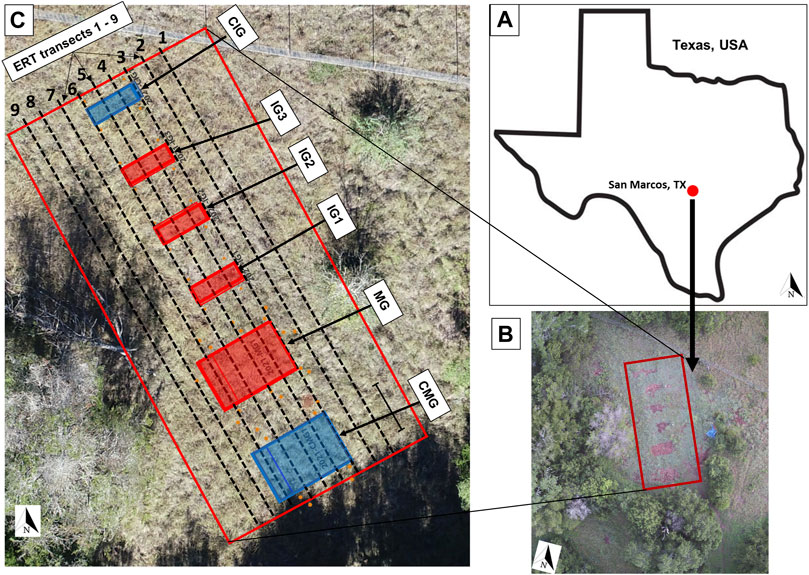
FIGURE 1. Location of the study site (A), an aerial view of the site taken by a drone, (B) and outline of graves and ERT profile lines 1–9 (C). CMG is control mass graves, MG is mass grave, IG1-3 are individual graves 1–3 and CIG is control individual grave.

The Freeman Ranch is characterized by a humid, sub-tropical climate with occasional drought leading to semi-arid conditions. Temperatures range from summer highs of 40°C to winter lows of 4°C, while average annual precipitation is estimated at 860 mm (Dixon, 2000). The shallow subsurface consists generally of topsoil with clayey–silty sediments overlying weathered dolomite and fractured limestone bedrocks (Carson, 2000; Fancher et al., 2017). The vegetation at the site is dominated by perennial grasslands invaded by Ashe juniper (Aitkenhead-Peterson et al., 2021). The site generally consists of two well-drained stony soils formed by weathering of the dolomitic limestone and indurated fractured limestone which constitute the shallow bedrock in the area. The soil zones in the area consist majorly of the Comfort-Rock and the Rumple-Comfort soils. The Comfort-Rock soils has 1%–8% slopes and comprise extremely stony clay at 0–33 cm, while the Rumple-Comfort soils are made up of gravelly loamy–clay from 0 to 25 cm followed by very gravelly clay from 25 cm.

Experimental setup

This study is part of a multidisciplinary and international forensic research project to investigate post-burial changes within a mass grave experimental context (Doro et al., 2022). The experimental setup involves a mass grave with six human cadavers, a control mass grave of the same dimensions without human cadavers, three individual graves with one human cadaver each, and a control individual grave without human cadavers (Figure 1). Prior to the excavation of the mass grave, individual graves, and control graves, background measurements of parallel 2D transects of electrical resistivity (Figure 1) were conducted. Details on field methods and the equipment used are presented in the Methods section.

Two pits measuring 3.0 by 2.0 m wide and 0.8 m deep were excavated using a Berger excavator. One of the pits serves as a mass grave and contains donated human bodies while the other serves as a control and was backfilled without bodies (Figure 2). Six willed-donated bodies were placed simultaneously in the mass grave pit in a fresh stage of decomposition. The bodies were clothed and placed in direct contact with each other in a comingled fashion. Four additional pits measuring 2.0 m by 0.6 m wide and 0.8 m deep were excavated at the same time which serve as individual and control graves. A single willed-donated body was buried in three of the individual graves at the same time as the placement of the mass grave while the fourth served as the control grave and was backfilled with no human remains. The individual graves were used for comparing results between mass and single graves. In total, the experimental setup consists of six graves, with four containing human remains and two serving as control graves (Figures 1, 2).

FIGURE 2

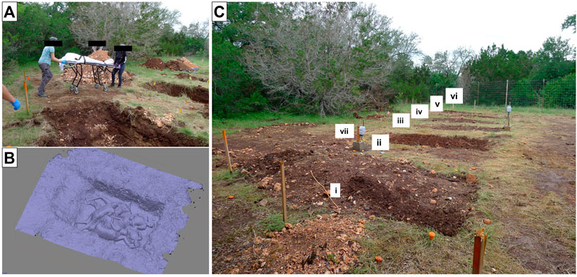
FIGURE 2. Experimental setup with (A) excavated graves and human remains being wheeled to the site, (B) a 3D model of the mass grave with six human cadavers created from photos, (C) outline of all six graves with (i) the control mass grave with no human cadaver, (ii) mass grave with six human cadavers deposited randomly, (iii, iv, and v) individual graves with one human cadaver each, (vi) control individual grave without cadavers, and (vii) one of three in situ Wi-Fi-enabled soil data loggers.

Prior to placing the bodies in the graves, the exposed soils were inspected for textural properties. After placing the bodies in the graves, industrial-grade in situ soil sensors capable of simultaneously measuring soil moisture, temperature, and electrical conductivity were placed at different locations and depths of the graves.

Methods

This study applies both forward numerical simulation and field time-lapse 2D and quasi-3D ERT investigations to image the experimental graves. Soil conditions were monitored continuously using in situ soil sensors. The details of each method are presented below.

Forward 2D electrical resistivity simulation

To design an appropriate field resistivity measurement setup, we first assessed the capability of different electrode arrays and unit electrode spacings for measuring the contrast between graves with human remains and empty control graves arranged in a parallel sequence and contrast between the graves and their surrounding undisturbed soils. A 3-layer forward resistivity model was developed to mimic the general shallow subsurface geology of the area which consists of clay-rich topsoil, a weathered bedrock zone, and dolomite bedrock. Resistivity values of 40, 100, and 500 Ωm were assigned to the layers in a top to bottom sequence. Six graves were established within the topsoil and weathered layer zone extending to a depth of 80 cm and dimensions mimicking the experimental setup. A resistivity of 10 Ωm was used for the mass grave and three individual graves with human remains, while that of 20 Ωm was used for the control mass and individual grave (Figure 3—top row). The resistivity values reflect literature values for the soil and rock types while we assume much lower resistivity in the graves to simulate the effect of conductive leachate and preferential accumulation of soil moisture in the graves, while values of the control graves are used to mimic only moisture accumulation effects.

FIGURE 3

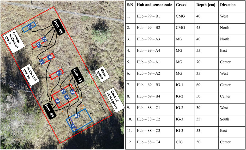
FIGURE 3. Outline of the graves and location of each of the soil sensors. Both position and installation depth of each sensor is presented in a tabular form on the right.

We used a 2D finite element–based forward solution R2 resistivity code implemented in ResIpy (Blanchy et al., 2021) to simulate the apparent resistivity distribution resulting from the created model using 0.25-, 0.5-, 0.75-, and 1.0-m unit electrode spacings and dipole–dipole and Wenner and Schlumberger electrode configurations. We added five percent white noise to the calculated apparent resistivity to mimic field errors and inverted the data using the Gauss–Newton–based inverse solution implemented in the same code (Binley and Kemna, 2005; Binley and Slater, 2020).

Field electrical resistivity measurement

For this study, we acquired repeated field measurements of electrical resistivity data in five different campaigns referred here as pre-burial and post-burial 1–5 with data acquisition carried out on 10 May, 15 May, 19 June, 23 July, and 14 November 2021, respectively. Data acquisition was carried out using an eight-channel R8 Supersting resistivity meter (AGI USA, Austin, TX, United States) with a multielectrode switchbox which allows for automatic switching of up to 84 current and potential electrodes. We acquired nine parallel transects spaced 1 m apart with transects 4 and 5 cutting across all the graves and transect 6 cutting across only the mass graves, while other transects were outside the grave boundaries (Figure 1). The surveys were conducted with 42 stainless steel surface electrodes using a dipole-dipole electrode configuration, with a 0.5-m unit electrode spacing resulting in a profile length of 20.5 m. The choice of the electrode array and unit electrode spacing was based on assessed trade-offs between data acquisition time and sensitivity to the potential temporal resistivity changes.

With the distance between profiles maintained at 1 m, five resistivity transects (ERT transects 1–5 in Figure 1) were acquired for the study prior to the excavation of the graves, while all nine transects were acquired for each of the post-burial survey to cover the study domain of 20.5 m × 8 m. Each transect took about 45 min to be set up. For each measurement, we used the current injection duration of 1.2 ms and three measurement cycles with the measurement error set at 2%. A total of 477 apparent resistivity data points were acquired along each transect which took about 15.2 min. While the resistivity data were acquired individually across each transect in a 2D framework, we combined all five transects for the pre-burial survey and all nine transects in each subsequent post-burial measurement cycle to generate a quasi-3D dataset following the rule that the distance between each transects is not more than twice the unit electrode spacing (Doro et al., 2013). Besides the regular nine 2D transects acquired using a dipole–dipole array and unit electrode spacing of 0.5 m, we also acquired measurement across transects 4 and 5 using a 0.25-m electrode spacing during post-burial 3 and 4 surveys. While data acquisition with the 0.5-m unit electrode spacing required only 42 electrodes to be laid out with an acquisition time of 15.2 min, using a unit electrode spacing of 0.25 m required laying out 84 electrodes and an acquisition time of 57.4 min using an eight channel multielectrode resistivity meter.

We first inverted the 2D and quasi-3D resistivity datasets using the same inversion framework in ResIPy to generate 2D and 3D resistivity distributions for each of the five measurement time steps (referred to as pre-burial, and post-burial 1, 2, 3, and 4) and used Paraview software to visualize the 3D results. We later carried out a time-lapse resistivity inversion using a difference inversion approach (LaBrecque and Yang, 2001; Binley and Kemna, 2005; Hayley et al., 2011) for the 2D datasets to highlight the difference in resistivity between each successive timestep. For transects 1–5, the pre-burial measurements were taken as the background resistivity data, while for transects 6–9, the post-burial 1 measurement was assumed as the background resistivity data.

Soil characterization and sensors

After excavation and prior to burying the human cadavers in the pits, we conducted a characterization of the soil exposed at each of the grave pits by observing their texture, color, and other physical properties. More details on the soil characterization are presented by Doro et al. (2022). To assess changes in the soil properties with time, industrial-grade MODBUS-RTU RS485 (Seed Studio, Hong Kong) soil sensors were installed at different depths in each of the graves (Figure 3). Each sensor measures soil electrical conductivity, temperature, and moisture content. A total of twelve sensors were installed in the graves and were connected to three different battery-powered, WiFi-enabled data loggers (hubs -69, -88, and -99, Figure 3), which allowed for remote data access.

Results

The conceptual resistivity model used for the forward simulation is shown in the first row of Figure 4, while the inversion results of the synthetic data showing resistivity distribution in logarithmic scale for the different unit electrode spacings and electrode arrays are presented below. Generally, the synthetic model inversion results capture the low resistive graves in the top layer as discontinuous low-resistivity zones in all cases with different unit electrode spacings and configurations with values similar to what we defined in the conceptual model. The model results show an overestimation of the resistivity of the graves at the edges by over 10%. While the structure of the graves is conserved in all cases with smoothening of the edges, the dipole–dipole shows the least contrast for the simulated control graves. In addition, reducing the unit electrode spacing increases the resolution of the low-resistivity anomaly representing the graves. However, a unit electrode spacing of 1 m sufficiently captures the low-resistivity anomalies representing the graves.

FIGURE 4

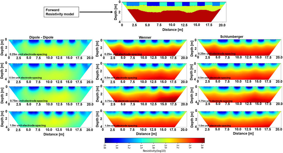
FIGURE 4. Comparison of results from multiple forward simulation scenarios. Row 1 shows the conceptual model with the resistivity distribution and outline graves. Columns 1, 2, and 3 show results for simulation using dipole–dipole, Wenner, and Schlumberger electrode configurations, respectively, while rows 2, 3, 4, and 5 show simulation using 0.25-, 0.5-, 0.75-, and 1.0-m electrode configurations, respectively.

The results of 2D distribution of resistivity for pre-burial and post-burial 1–4 measurements for transects 3 and 4 are shown in Figure 5, while those for transects 5 and 6 are shown in Figure 6. These selected 2D transects are presented for this study as they are in the region with the graves (Figure 1). In all inversion scenarios, the resistivity model converged after three to four iterations with a root mean square (R.M.S) error value less than 1 and the normalized error model ranging from −2 to 2. Prior to excavation and establishment of the graves, the resistivity distributions for transects 3–5 (Row 1 of Figures 5, 6) show a 3-layer resistivity model with the resistivity increasing in a top to bottom sequence. The top layer has a very low resistivity ranging from 0.8 to 1.4 Ωm on the log (10) scale down to a depth range of 0.4–0.7 m and transition through a medium-resistivity layer ranging from 1.4 to 1.9 Ωm on the log (10) scale at a depth range of 0.7–1.5 m. These layers are underlain by a high resistivity >2.0 Ωm on the log (10) scale. These values are consistent across profiles 4 and 5 with similar structure, except that the transition zone is deeper at about 3.5 m (at the left side) of profile 4.

FIGURE 5

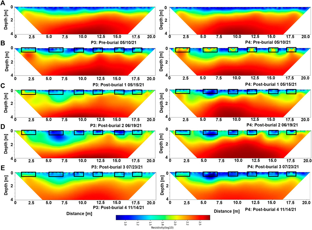
FIGURE 5. 2D distribution of electrical resistivity across graves for profiles 3 (left) and 4 (right). Five different measurements were conducted (A) prior to burial, (B) 2 days after burial, (C) 1 month after burial, (D) 2 months after burial, and (E) 6 months after burial.

FIGURE 6

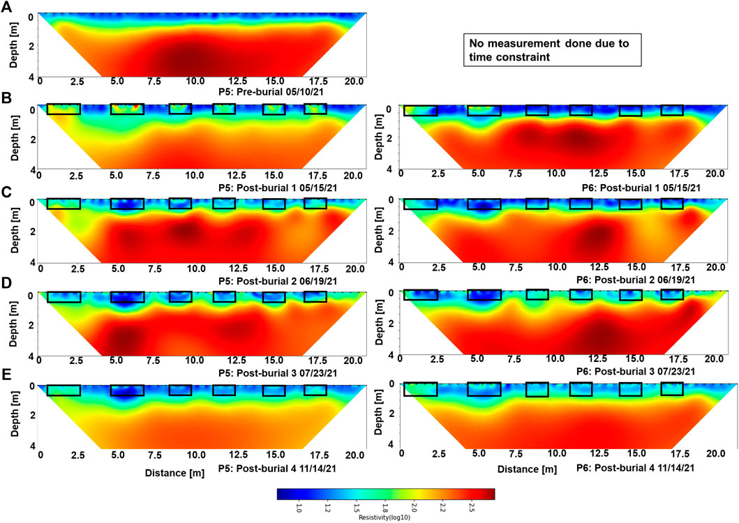
FIGURE 6. 2D distribution of electrical resistivity across graves for profiles 5 (left) and 6 (right). Five different measurements were conducted (A) prior to burial, (B) 2 days after burial, (C) 1 month after burial, (D) 2 months after burial, and (E) 6 months after burial.

Resistivity distributions measured 2 days after burial show consistently higher resistivity for profiles 4–6 (Figures 5, 6) at regions corresponding to graves containing human remains and the control graves with no human remains. A resistivity increase of up to 50% is measured with higher values around the control graves. For resistivity measured 1, 2, and 6 months after burial, lower resistivities are measured around all the graves with stronger decrease of about 40% around the mass grave where six human remains were deposited. While resistivity decreases with time after burial in all graves with human remains, the decrease is stronger in the mass grave. The low-resistivity anomaly at the mass grave location shows a downward migration down to a depth of 1.2 m compared to the original grave depth of 0.8 m (Profiles 4 and 5 in Figures 5, 6). A stronger resistivity contrast is observed between the grave and surrounding areas for post-burial 1 and 3 compared to 2 and 4.

3D resistivity distribution for all five different measurement time steps (pre-burial, and post-burials 1–4) are shown in Figure 7, with a vertical and depth slice at 2 × 2 m for pre-burial result and 4 × 2 m for results of post-burial 1–4 to better visualize the grave outline. A volume rendering highlighting resistivity anomalies at the upper 1 m where the grave is located is shown in Figure 7 (column 3). The 3D inversion for all cases also converged after four iterations, with R.M.S. error values ranging from 0.8–1.5 and the normalized error range between −3 and +3. While the 3D results show similar resistivities as the 2D images, the 3D volume shows the grave outlines as high-resistivity zones for post-burial 1 (2 days after burial) and low-resistivity zones for post-burial 3 (71 days after burial). 3D volume results for measurements acquired 1 and 6 months after burial do not show the outline of the graves from a top view but are revealed when the resistivity volume is sliced laterally at 4 and 2 m depth. The low-resistivity anomaly is, however, weaker in areas around the graves than anomaly measured 2 months after burial. The volume rendering in column 3 of Figure 7 also highlights resistivity anomalies in a 3D volume form that corresponds to the graves for measurement acquired 2 days and 2 months after burial.

FIGURE 7

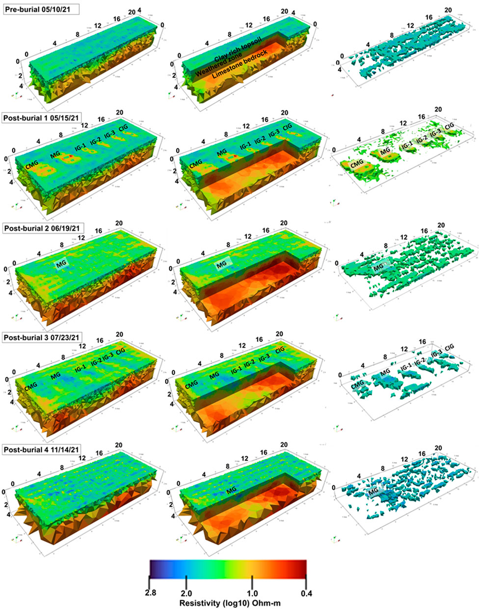
FIGURE 7. Quasi-3D resistivity distribution obtained by merging nine 2D transects and inverting with a 3D inversion code. The complete resistivity volume showing the outlines of the graves visible in post-burial 1 and 3 (rows 2 and 3) are show in column 1, the 3D volume sliced at 2 m × 4 m is shown in column 2 while a volume rendering highlighting 3D anomalies produced by the grave is shown in column 3.

The results of time-lapse resistivity inversions for transects 4 and 5 showing resistivity changes with time referenced to background measurement acquired prior to excavation are presented in Figure 8. The results show up to 60% increase in resistivity for measurement made 2 days after burial (post-burial 1), with changes higher in the control graves. Thereafter, the resistivity within the graves decreases up to—70% with the highest decrease measured in the mass grave. Positive changes in resistivity for measurement acquired 2 days after burial are confined to the known grave boundaries. Besides the mass grave, there is no significant change in resistivity for measurement conducted 1 month after burial. While resistivity generally decreases with time after burial for time-lapse results from 2 to 6 months after burial, the decrease is stronger at the mass grave. The observed decrease in resistivity around the mass grave region for measurements acquired 2 months after burial extends downward to a depth of about 1.5 m. A similar downward extension of the resistivity decrease is also observed in the time-lapse result for the measurement conducted 6 months after burial in both the mass and individual graves.

FIGURE 8

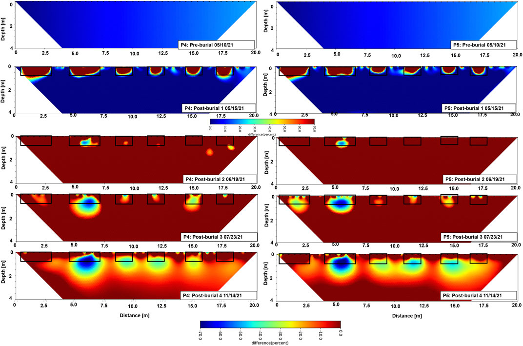
FIGURE 8. 2D time-lapse resistivity distribution of for transects 4 (left) and 5 (right) cutting across all graves. Percentage changes were calculated as the difference between the original measurements on undisturbed ground minus the measurements over the burials, divided by the original measurements. It is to be noted that the scale for the top rows is limited to negative values, while that for the bottom profiles shows positive values.

The 2D resistivity distribution for field measurements along profiles 4 and 5 for post-burial 3 (acquired 2 months after burial) using 0.5- and 0.25-m unit electrode spacing is shown in Figure 9. The model shows improvement in resolving the structure of the low-resistivity anomaly in the graves with buried human remains for both profiles. A thin high-resistivity structure can be observed overlying the low-resistivity structure for the measurements with smaller electrode spacing of 0.25 m, particularly in the mass grave.

FIGURE 9

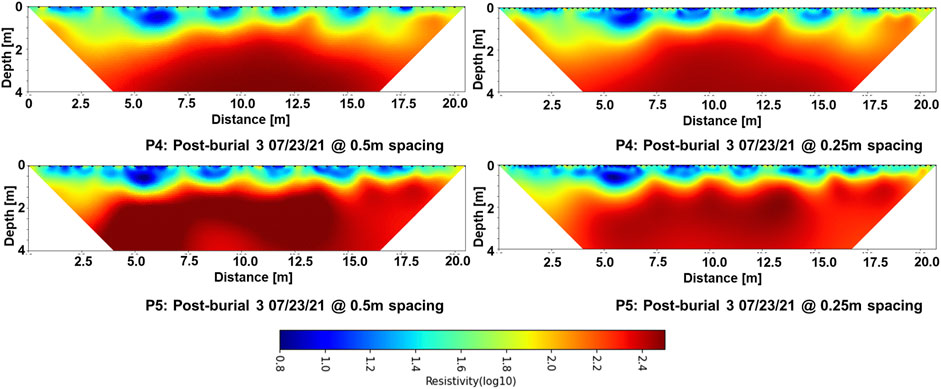
FIGURE 9. Comparison of 2D resistivity distribution for transects 4 (top) and transect 5 (bottom) with data acquired using a unit electrode spacing of 0.5 m (left) and 0.25 m (right).

Soil exposed at the excavated graves down to depth 80 cm show mainly three different horizons with the top 0.2 m consisting of loose, dark reddish-brown clay–loamy soil with relatively high organic matter dominated by plant roots and large angular-to-subangular rock fragments which are likely products of in situ weathering of the bedrock. The second horizon extends from 0.2–0.5 m and is similar to the overlying horizon but has higher moisture and clay content, is more plastic, and has a lighter shade of reddish-brown coloration with whitish material suspected to be calcite. The third horizon extends to a depth of 0.7–0.8 m and consists of highly weathered limestone which is a typical bedrock in the area. The observed three soil horizons are underlain by a limestone bedrock. While observed soil types and properties were similar at all six excavated locations, they show variations in the pebble and cobble contents, color, the degree of weathering at the third horizon, and the depth to basement which is shallower (depth to bedrock of 70 cm) at the northern segment of the test site.

Changes in soil electrical conductivity, temperature, and volumetric water content measured with the in situ sensors in each of the graves for over 6 months after burial are shown in Figure 10. Electrical conductivity in the mass grave shows a sharp increase in the first 75 days after burial up to 5.2 mS/cm and thereafter, the values decreased gradually to 3.5 mS/cm around 190 days after burial. Soil electrical conductivity is similar in all three individual graves with the average values much lower than those measured in the mass grave with an average range of 0.7–1.9 mS/cm and spikes of up to 2.2 mS/cm corresponding to a period of intense rainfall. Soil temperatures show a similar trend in all the graves with higher values (40°C) measured in the summer and lower values (18°C) in late fall. Soil volumetric water content (VWC) shows a similar temporal trend in all graves with a range of 20%–50 % except for the mass grave where a sharp increase in soil moisture content was observed in the first 60 days post burial and reaching saturation (100%) thereafter. A slight decreasing trend is seen after 180 days to values at 98 percent.

FIGURE 10

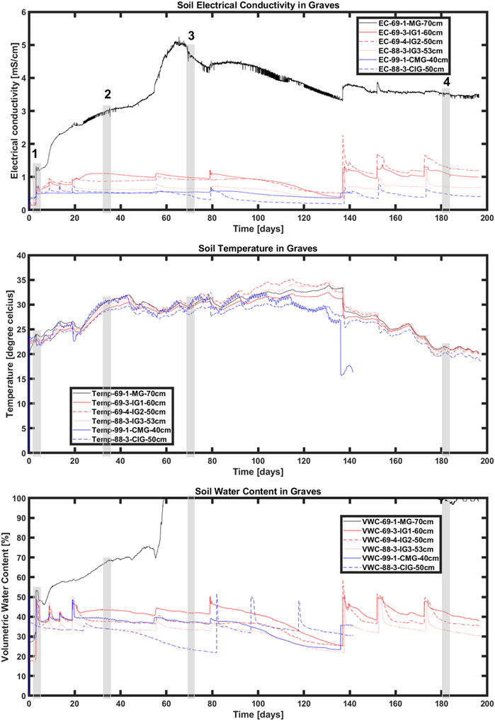
FIGURE 10. Soil electrical conductivity (top row), temperature (middle row), and volumetric moisture content (bottom row) measured in the mass grave. Highlighted locations 1 to 4 are dates when post-burial geophysical measurements were conducted.

Discussion

Forward modeling of electrical resistivity was used in this study to calculate the resistivity distribution that is expected, given the subsurface structure and simulated graves using the dipole–dipole, Wenner and Schlumberger arrays, and electrode spacing ranging from 0.25 to 1 m. Hence, it allowed us to plan the field resistivity measurements and decide optimum trade-off between field constraints such as measurement time and the desired sensitivity (Binley and Slater, 2020). Our forward modeling results show that the dipole–dipole and Wenner and Schlumberger arrays successfully delineate the low-resistivity zones, mimicking the graves with human remains and the empty controls (Figure 4). Although the dipole–dipole array underestimates the high-resistivity unit representing the bedrock and may be susceptible to smoothening at the edge, it offers a unique advantage of a faster data acquisition time using the same equipment and number of electrodes. For this study, using 42 electrodes at 0.5 m spacing with an eight-channel Supersting R8 resistivity meter (AGIUSA Texas, United States), the dipole–dipole took 15 min to acquire 477 data points compared to the Wenner array which took 57 min to acquire 273 data points. With dipole–dipole being significantly sensitive to the low-resistivity anomaly at the top 1 m, we decided to use it in this study, trading the advantage of fast data acquisition time for improved sensitivity to the bedrock layer which is not the focus of the imaging in this study. This allows us to acquire all nine transects at each of our repeated multigeophysical campaign. However, the forward modeling result shows that where time is not a constraint, the Schlumberger array provides a better sensitivity to the soil and bedrock units down to 4 m. Our forward modeling result also reveals that unit electrode spacings of 0.25, 0.5, 0.75, and 1 m successfully delineated the low-resistivity units mimicking both individual and mass graves. Nevertheless, increasing the unit electrode spacing resulted in slight decrease in the resolution of the anomalies from the simulated graves.

Previous studies using ERT to monitor simulated graves have mainly used the Wenner electrode array and unit electrode spacing ranging from 0.25 to 1 m (Pringle et al., 2012; Molina et al., 2016; Cavalcanti et al., 2018). Pringle et al. (2012) presented a first of such study which compared field measurements using dipole–dipole and Schlumberger and Wenner arrays and concluded that the Wenner array was more optimal though they did not show how such an optimum tradeoff was reached. Cavalcanti et al. (2018) compared results using both Wenner and Schlumberger arrays and concluded that both show similar sensitivity to the shallow subsurface where the graves were established, but the Wenner array provided an overall better vertical resolution. Both Pringle et al. (2012) and Cavalcanti et al. (2018) also emphasized the need for smaller unit electrode spacing of 0.25 and 0.5 m, respectively to improve the resolution of the grave features. These studies, however, rely on field observations and comparisons for their post-measurement deductions. We propose integrating a forward modeling approach to efficiently establish the optimum tradeoff. Indeed, our forward modeling results suggest the dipole–dipole array with a unit electrode spacing of 0.5 m as an optimum tradeoff where time is a constraint and given a modern multichannel acquisition system. Forward simulations should, however, be used to guide such decisions when necessary, considering unique site properties.

The three-layer resistivity model seen in the resistivity data acquired prior to excavation (top row in Figures 5, 6) corresponds to the top clay-rich topsoil, the weathered bedrock, and the limestone bedrock observed in the grave pit. The deeper middle-resistivity zone also corresponds to a deeper weathered bedrock zone observed during the excavation with a greater ease of excavation down to about 1 m. The results of 2D resistivity measurements acquired 2 days after burial captures all the graves including the controls as high-resistivity zones (Figures 5, 6, row 2). We attribute these high resistivities to effects of soil disturbances caused by excavation and backfilling. The soils in the graves were aerated during excavation and backfilling with the air-filled pores becoming more resistive (Sauer et al., 2014; Yurkevich et al., 2021) than that of the surrounding undisturbed soil. The preferential aeration within the grave will last until subsidence enhanced by rainfall cause the soil to settle. Cavalcanti et al. (2018) and Pringle et al. (2008) reported that resistivity generally decreases after burial. It should, however, be noted that both studies did not show resistivity results acquired immediately (a few days) after burial which would have allowed for a more appropriate comparison with the result of this study. While it is thought that the process of soil excavation and backfilling during the establishment of a grave increases the soil porosity within the grave (Scott and Hunter, 2004; Jervis et al., 2009), which should result in decrease in resistivity following the petrophysical model developed for saturated medium (Henry, 1997; Choo et al., 2016; Cai et al., 2017), our results acquired 2 days after burial show an opposite trend with an increase in resistivity observed in all graves including the control graves.

Post-burial resistivity results measured 1, 2, and 6 months after burial generally show decreasing resistivities in all the graves with stronger decreases in the graves with human remains and the decrease highest in the mass grave. The decrease is more rapid for the first 2 months than 6 months after burial (Figures 5, 6). We interpret the decrease in resistivities to result from 1) preferential infiltration within the graves, resulting in an increasing soil water content and 2) decay of the human cadavers which would have produced a conductive leachate from liquified soft tissues. Hence, with only the effect of infiltration expected within the control graves, their resistivity decrease should be less than the corresponding decrease in the graves with human remains where both increase in soil water content and conductive leachate from decay contribute to the observed resistivity decrease. This is, indeed, what our data over a 6-month period show.

Resistivity changes in graves with human remains after burial could be subtle and difficult to quantify if we rely only on direct comparison of successive timesteps. Time-lapse inversion results shown in Figure 8 visualize the resistivity changes attributed to the graves in comparison with measurements made prior to burial taken as the background resistivity. The time-lapse inversion results emphasize the stronger low-resistivity anomaly around the mass grave than that of the single graves, making resistivity even more viable for locating mass graves. In addition, while results of measurements acquired 1 and 6 months after burial do not show significant changes in regions with the graves (Figures 5–7), which would make it difficult to identify them in a blind study, the time-lapse results (Figure 8) show changes in resistivity when compared to the background. This makes the grave identifiable in the 2D resistivity images. Although time-lapse measurement may not always be feasible due to time and logistical constraints during the search for clandestine individual or mass graves, time-lapse studies can provide support for human decomposition research because they can relate to the temporal processes of decay.

The 3D resistivity model shown in this study allows a volumetric visualization of the resistivity anomalies attributed to the graves and improves the delineation of their dimensions. The 3D model offers a unique advantage of providing additional information on the lateral and depth extent of the graves. The resistivity volume rendering in Figure 7 (column 3) particularly highlights resistivity anomalies as 3D shapes corresponding to the graves for measurement carried out 2 days and 2 months after burial but not for measurements carried out 1 and 6 months after burial. The difficulty in identifying the grave for measurements acquired 1 and 6 months after burial is due to the presence of multiple anomalies in the model not related to the graves that make identifying the graves difficult. This effect can be associated with the decrease in sensitivity of the quasi-3D resistivity models described as pseudo 3D models by Yang and Lagmanson (2006) compared to a true 3D model. While this provide an argument in favor of testing a true 3D data acquisition in a forensic context to assess its value, it should be noted that such true 3D data acquisition is resource-intensive, requiring more field electrodes, suitable instrumentation, and data acquisition and processing times.

A comparison of the results of 2D resistivity distribution using 0.5- and 0.25-m unit electrode spacing (Figure 9) show improvement in the resolution of the resistivity anomaly resulting from the graves when a smaller unit electrode spacing is used. The structure of the anomaly is better resolved with a thin high-resistivity structure overlying a low-resistivity structure. The high-resistivity structure can be interpreted as the backfilled soil layer overlying the buried bodies. While such improvement in resolution is useful, it is important to note that the data acquisition time and effort increases by a factor of 4. While data acquisition with 0.5-m unit electrode spacing would require only 42 electrodes to be laid out with an acquisition time of 15.2 min, using a unit electrode spacing of 0.25 m would require laying out 84 electrodes and an acquisition time of 57.4 min and twice the setup time.

Generally, 2D and quasi-3D resistivity results in this study clearly show locations of the graves with identifiable resistivity anomalies over time demonstrating the efficacy of resistivity as a noninvasive forensic search tool for locating clandestine graves and supporting human decomposition research. The measured anomalies, however, show temporal variations with the individual graves not easily identifiable in the 2D and 3D models for data acquired 1 and 6 months after burial. The changes in soil electrical conductivity, temperature, and volumetric water content (Figure 10) show variations which may partially account for this temporality in the resistivity signals. Measurement carried out 2 months after burial matches a time when soil moisture, temperature, and water contents were high corresponding to a strong resistivity contrast in the graves, while measurement carried out 6 months after burial matches time with comparatively lower temperatures and electrical conductivities and low-resistivity contrast between the graves and surrounding soils. Jervis and Pringle (2014) and Pringle et al. (2016) showed that the measured resistivity in graves varies with soil moisture and precipitation volume. While our study appears to support this conclusion, measuring the soil properties over a longer duration as planned in this study and comparing that with weather data for a similar time range will help us effectively compare the temporality in measured resistivity anomalies with changes in soil properties and climate variables.

Conclusion

This study validates the potential of 2D and 3D ERT as a noninvasive tool for forensic scientists in the search for clandestine mass and individual graves and as an imaging technique to support human decomposition research. We used both forward numerical simulation and field measurement of 2D and quasi-3D electrical resistivity to image the graves and assess the effects of disturbed ground and the presence of decaying human remains and conductive decomposition products within the graves. The measured resistivity anomaly is higher in the case of the mass grave with multiple human remains than in the individual graves containing single cadavers. This confirms stronger capability of electrical resistivity in isolating anomalies associated with mass graves than individual graves.

Forensic applications of ERT remain limited because it takes more time to collect data than other geophysical methods such as GPR or electromagnetic imaging, and it requires fixing electrodes to the soil which is not possible in built-up areas and where the surface is covered with concrete or asphalt. However, ERT should not be dismissed as unsuitable for forensic investigations especially in light of advances in instrumentation that address some of these shortcomings. For example, state-of-the-art multichannel acquisition equipment such as the equipment used in this study can measure potentials between several pairs of electrodes simultaneously during the same current injection, which significantly decreases the time to collect data; mobile-probe arrays such as the Geoscan RM85 with PA20 frame or MSP40 platform (Geoscan Research, Clayton UK) allow for more rapid covering of a survey area and capacitively coupled electrodes such as the Ohm Mapper technology (Geometrics, San Jose, California) provide an alternative where classical electrodes cannot be attached to the ground. A subsequent study could compare aspects of acquisition and imaging for various methods and different types of equipment applied at a forensic test site. At minimum, our results prove that ERT can serve as a useful follow-up technique for a more targeted investigation after an initial scanning with GPR and before excavations are carried out on potential burial anomalies, especially where anomalies detected in GPR seem ambiguous or the ground produces a lot of scatters in the radar data.

Our results show the usefulness of forward modeling of resistivity data before data collection. Typically, ERT results are based on data collected along lines of equally spaced electrodes and using standard injection-measurement pairs (e.g., dipole–dipole, Wenner, and Schlumberger). Forward modeling in this study allowed us to select spacing and array type based on optimal efficiency. We envision that such a forward modeling approach can be extended to real 3D resistivity data acquisition, using a grid of electrodes as opposed to the standard lines and unconventional electrode setups. The approach may further be extended to applying machine learning during data acquisition to guide the optimal electrode arrangement given the already measured data. The potential for ERT has not been exhausted and in our opinion continues to hold promise for forensic searches.

Data availability statement

The raw data supporting the conclusion of this article will be made available by the authors, without undue reservation.

Author contributions

KD, C-GB, DW, and HM contributed to conception and design of the study. KD and C-GB planned the geophysical data acquisition. KD, EE, and MA acquired and processed field data. KD and MA carried out forward and inverse modeling. KD wrote the first draft of the manuscript. KD, C-GB, DW, and HM wrote sections of the manuscript. All authors contributed to manuscript revision and read and approved the submitted version.

Funding

Financial support was provided by the University of Toledo, Ohio to KD as research start-up funds.

Conflict of Interest

The authors declare that the research was conducted in the absence of any commercial or financial relationships that could be construed as a potential conflict of interest.

Publisher’s Note

All claims expressed in this article are solely those of the authors and do not necessarily represent those of their affiliated organizations, or those of the publisher, the editors, and the reviewers. Any product that may be evaluated in this article, or claim that may be made by its manufacturer, is not guaranteed or endorsed by the publisher.

Acknowledgments

We acknowledge the collaborative efforts of the members of the experimental mass grave research team for their support and Akinwale Ogunkoya and Amar Kolapkar, students at the University of Toledo who assisted with field data acquisition.

References

Abate, D., Sturdy Colls, C., Moyssi, N., Karsili, D., Faka, M., Anilir, A., et al. (2019). Optimizing Search Strategies in Mass Grave Location through the Combination of Digital Technologies. Forensic Sci. Int. Synergy 1, 95–107. doi:10.1016/j.fsisyn.2019.05.002

PubMed Abstract | CrossRef Full Text | Google Scholar

Aitkenhead-Peterson, J. A., Fancher, J. P., Alexander, M. B., Hamilton, M. D., Bytheway, J. A., and Wescott, D. J. (2021). Estimating Postmortem Interval for Human Cadavers in a Sub-tropical Climate Using UV-Vis-Near-Infrared Spectroscopy. J. Forensic Sci. 66 (1), 190–201. doi:10.1111/1556-4029.14579

PubMed Abstract | CrossRef Full Text | Google Scholar

Barker, C., Alicehajic, E., and Naranjo, S. J. (2017). “Post‐mortem Differential Preservation and its Utility in Interpreting Forensic and Archaeological Mass Burials,” in Taphonomy of Human Remains: Forensic Analysis of the Dead and the Depositional Environment: Forensic Analysis of the Dead and the Depositional Environment, 251–276.

Google Scholar

Bawallah, A. M., Ilugbo, S. O., Adebo, B. A., and Kehinde, O. A. (2021). Geophysical Investigation for Detecting Buried Human Remains after Eight Years of Burial in Owo, Southwestern Nigeria. J. Forensic Sci. 67 (2), 786–794. doi:10.1111/1556-4029.14923

PubMed Abstract | CrossRef Full Text | Google Scholar

Bentley, L. R., and Gharibi, M. (2004). Two‐ and Three‐dimensional Electrical Resistivity Imaging at a Heterogeneous Remediation Site. Geophysics 69 (3), 674–680. doi:10.1190/1.1759453

CrossRef Full Text | Google Scholar

Berezowski, V., Keller, J., and Liscio, E. (2018). 3D Documentation of a Clandestine Grave: a Comparison between Manual and 3D Digital Methods. J. Assoc. Crime Scene Reconstr. 22, 23–37. Available at: https://www.acsr.org/wp-content/uploads/2018/12/2018-3D-Documentation-of-Clandestine-Graves-Berezowski.pdf

Google Scholar

Berezowski, V., Mallett, X., Ellis, J., and Moffat, I. (2021). Using Ground Penetrating Radar and Resistivity Methods to Locate Unmarked Graves: A Review. Remote Sens. 13 (15), 2880. doi:10.3390/rs13152880

CrossRef Full Text | Google Scholar

Binley, A., and Kemna, A. (2005). Hydrogeophysics. Editors Y. Rubin, and S.S. Hubbard (Dordrecht, Springer Netherlands), 129–156.

Google Scholar

Binley, A., and Slater, L. (2020). Resistivity and Induced Polarization: Theory and Applications to the Near-Surface Earth. Cambridge CB2 8BS, United Kingdom: Cambridge University Press.

Google Scholar

Blanchy, G., Saneiyan, S., Boyd, J., McLachlan, P., Binley, A., and Blanchy, G. (2021). ResIPy: An Intuitive Open Source Software for Complex Geoelectrical Inversion/Modeling. Amsterdam: European Association of Geoscientists & Engineers, 1–2.

Google Scholar

Cai, J., Wei, W., Hu, X., and Wood, D. A. (2017). Electrical Conductivity Models in Saturated Porous media: A Review. Earth-Science Rev. 171, 419–433. doi:10.1016/j.earscirev.2017.06.013

CrossRef Full Text | Google Scholar

Carson, D. (2000). Soils of the Freeman Ranch, Hays County, Texas. San Marcos, TX: Freeman Ranch Publication. Series-No. 4-2000.

Google Scholar

Cavalcanti, M. M., Rocha, M. P., Blum, M. L. B., and Borges, W. R. (2018). The Forensic Geophysical Controlled Research Site of the University of Brasilia, Brazil: Results from Methods GPR and Electrical Resistivity Tomography. Forensic Sci. Int. 293, 101.e1–101.e21. doi:10.1016/j.forsciint.2018.09.033

PubMed Abstract | CrossRef Full Text | Google Scholar

Choo, H., Song, J., Lee, W., and Lee, C. (2016). Impact of Pore Water Conductivity and Porosity on the Electrical Conductivity of Kaolinite. Acta Geotech. 11 (6), 1419–1429. doi:10.1007/s11440-016-0490-4

CrossRef Full Text | Google Scholar

Dargan, R., and Forbes, S. L. (2021). Cadaver-detection Dogs: A Review of Their Capabilities and the Volatile Organic Compound Profile of Their Associated Training Aids. WIREs Forensic Sci. 3 (6), e1409. doi:10.1002/wfs2.1409

CrossRef Full Text | Google Scholar

Dick, H. C., Pringle, J. K., Sloane, B., Carver, J., Wisniewski, K. D., Haffenden, A., et al. (2015). Detection and Characterisation of Black Death Burials by Multi-Proxy Geophysical Methods. J. Archaeological Sci. 59, 132–141. doi:10.1016/j.jas.2015.04.010

CrossRef Full Text | Google Scholar

Dixon, R. (2000). Climatology of the Freeman Ranch, Hays County, Texas. San Marcos, TX: Freeman Ranch Publication. Series 3, 1-9.

Google Scholar

Donnelly, L. (2021). A Standard Operating Procedure (SOP), for Soil Sampling, for the Detection of Volatile Organic Compounds and Leachate Associated with Human Decomposition from a Shallow, Unmarked, Homicide Grave. Geol. Soc. Lond. Spec. Publications 492 (1), 123–133. doi:10.1144/sp492-2020-58

CrossRef Full Text | Google Scholar

Donnelly, L., and Harrison, M. (2013). Geomorphological and Geoforensic Interpretation of Maps, Aerial Imagery, Conditions of Diggability and the Colour-Coded RAG Prioritization System in Searches for Criminal Burials. Geol. Soc. Lond. Spec. Publications 384 (1), 173–194. doi:10.1144/sp384.10

CrossRef Full Text | Google Scholar

Doro, K. O., Kolapkar, A. M., Bank, C.-G., Wescott, D. J., and Mickleburgh, H. L. (2022). Geophysical Imaging of Buried Human Remains in Simulated Mass and Single Graves: Experiment Design and Results from Pre-burial to Six Months after Burial. Forensic Sci. Int. 335, 111289. doi:10.1016/j.forsciint.2022.111289

PubMed Abstract | CrossRef Full Text | Google Scholar

Doro, K. O., Leven, C., and Cirpka, O. A. (2013). Delineating Subsurface Heterogeneity at a Loop of River Steinlach Using Geophysical and Hydrogeological Methods. Environ. Earth Sci. 69 (2), 335–348. doi:10.1007/s12665-013-2316-0

CrossRef Full Text | Google Scholar

Essefi, E. (2022). “Advances in Forensic Geophysics,” in Technologies to Advance Automation in Forensic Science and Criminal Investigation. Hershey, PA: IGI Global, 15–36. doi:10.4018/978-1-7998-8386-9.ch002

CrossRef Full Text | Google Scholar

Fancher, J. P., Aitkenhead-Peterson, J. A., Farris, T., Mix, K., Schwab, A. P., Wescott, D. J., et al. (2017). An Evaluation of Soil Chemistry in Human Cadaver Decomposition Islands: Potential for Estimating Postmortem Interval (PMI). Forensic Sci. Int. 279, 130–139. doi:10.1016/j.forsciint.2017.08.002

PubMed Abstract | CrossRef Full Text | Google Scholar

Feng, T., Su, W., Zhu, J., Yang, J., Wang, Y., Zhou, R., et al. (2021). Corpse Decomposition Increases the Diversity and Abundance of Antibiotic Resistance Genes in Different Soil Types in a Fish Model. Environ. Pollut. 286, 117560. doi:10.1016/j.envpol.2021.117560

PubMed Abstract | CrossRef Full Text | Google Scholar

Haglund, W. D. (2002). Advances in Forensic Taphonomy: Method, Theory, and Archaeological Perspectives. Editors W. D. Haglund, and M. H. Sorg (Boca Raton: CRC Press), 243–261.

Google Scholar

Hansen, J. D., and Pringle, J. K. (2013). Comparison of Magnetic, Electrical and Ground Penetrating Radar Surveys to Detect Buried Forensic Objects in Semi-urban and Domestic Patio Environments. Geol. Soc. Lond. Spec. Publications 384 (1), 229–251. doi:10.1144/sp384.13

CrossRef Full Text | Google Scholar

Hayley, K., Pidlisecky, A., and Bentley, L. R. (2011). Simultaneous Time-Lapse Electrical Resistivity Inversion. J. Appl. Geophys. 75 (2), 401–411. doi:10.1016/j.jappgeo.2011.06.035

CrossRef Full Text | Google Scholar

Henry, P. (1997). Relationship between Porosity, Electrical Conductivity, and Cation Exchange Capacity in Barbados Wedge Sediments. College Station, TX: National Science Foundation, 137–150.

Google Scholar

Jervis, J. R., Pringle, J. K., and Tuckwell, G. W. (2009). Time-lapse Resistivity Surveys over Simulated Clandestine Graves. Forensic Sci. Int. 192 (1), 7–13. doi:10.1016/j.forsciint.2009.07.001

PubMed Abstract | CrossRef Full Text | Google Scholar

Jervis, J. R., and Pringle, J. K. (2014). A Study of the Effect of Seasonal Climatic Factors on the Electrical Resistivity Response of Three Experimental Graves. J. Appl. Geophys. 108, 53–60. doi:10.1016/j.jappgeo.2014.06.008

CrossRef Full Text | Google Scholar

LaBrecque, D. J., and Yang, X. (2001). Difference Inversion of ERT Data: A Fast Inversion Method for 3-D In Situ Monitoring. Jeeg 6 (2), 83–89. doi:10.4133/jeeg6.2.83

CrossRef Full Text | Google Scholar

Li, M., Zhang, Z., Yang, J., and Xie, S. (2021). Integrated Geophysical Study in the Cemetery of Marquis of Haihun. Archaeological Prospection 28 (4), 453–465. doi:10.1002/arp.1815

CrossRef Full Text | Google Scholar

Mant, A. K. (1987). Death, Decay and Reconstruction: Approaches to Archaeology and Forensic Science. Editors A. Boddington, A. N. Garland, and R. C. Janaway (Manchester: Manchester University Press), 65–78.

Google Scholar

Mant, A. K. (1950). A Study in Exhumation Data. London: University of London.

Google Scholar

Martorana, R., Capizzi, P., and Carollo, A. (2018). Misinterpretation Caused by 3D Effects on 2d Electrical Resistivity Tomography-Tests on Simple Models. Amsterdam: European Association of Geoscientists & Engineers, 1–5.

Google Scholar

Mileto, C., Vegas López-Manzanares, F., Cristini, V., and Cabezos Bernal, P. M. (2021). Burial Architecture. 3D Dissemination Study for a Selection of Byzantine Graves. Virtual Archaeol. Rev. 12 (24), 90–98. doi:10.4995/var.2021.13187

CrossRef Full Text | Google Scholar

Molina, C. M., Pringle, J. K., Saumett, M., and Evans, G. T. (2016). Geophysical Monitoring of Simulated Graves with Resistivity, Magnetic Susceptibility, Conductivity and GPR in Colombia, South America. Forensic Sci. Int. 261, 106–115. doi:10.1016/j.forsciint.2016.02.009

PubMed Abstract | CrossRef Full Text | Google Scholar

Nero, C., Aning, A. A., Danuor, S. K., and Noye, R. M. (2016). Delineation of Graves Using Electrical Resistivity Tomography. J. Appl. Geophys. 126, 138–147. doi:10.1016/j.jappgeo.2016.01.012

CrossRef Full Text | Google Scholar

Pringle, J. K., Jervis, J., Cassella, J. P., and Cassidy, N. J. (2008). Time-Lapse Geophysical Investigations over a Simulated Urban Clandestine Grave. J. Forensic Sci. 53 (6), 1405–1416. doi:10.1111/j.1556-4029.2008.00884.x

PubMed Abstract | CrossRef Full Text | Google Scholar

Pringle, J. K., and Jervis, J. R. (2010). Electrical Resistivity Survey to Search for a Recent Clandestine Burial of a Homicide Victim, UK. Forensic Sci. Int. 202 (1), e1–7. doi:10.1016/j.forsciint.2010.04.023

PubMed Abstract | CrossRef Full Text | Google Scholar

Pringle, J. K., Jervis, J. R., Hansen, J. D., Jones, G. M., Cassidy, N. J., and Cassella, J. P. (2012). Geophysical Monitoring of Simulated Clandestine Graves Using Electrical and Ground-Penetrating Radar Methods: 0–3 Years after Burial*,†. J. Forensic Sci. 57 (6), 1467–1486. doi:10.1111/j.1556-4029.2012.02151.x

PubMed Abstract | CrossRef Full Text | Google Scholar

Pringle, J. K., Jervis, J. R., Roberts, D., Dick, H. C., Wisniewski, K. D., Cassidy, N. J., et al. (2016). Long-term Geophysical Monitoring of Simulated Clandestine Graves Using Electrical and Ground Penetrating Radar Methods: 4-6 Years after Burial. J. Forensic Sci. 61 (2), 309–321. doi:10.1111/1556-4029.13009

PubMed Abstract | CrossRef Full Text | Google Scholar

Pringle, J. K., Stimpson, I. G., Wisniewski, K. D., Heaton, V., Davenward, B., Mirosch, N., et al. (2021). Geophysical Monitoring of Simulated Clandestine Burials of Murder Victims to Aid Forensic Investigators. Geology. Today 37 (2), 63–65. doi:10.1111/gto.12344

CrossRef Full Text | Google Scholar

Pringle, J. K., Stimpson, I. G., Wisniewski, K. D., Heaton, V., Davenward, B., Mirosch, N., et al. (2020). Geophysical Monitoring of Simulated Homicide Burials for Forensic Investigations. Sci. Rep. 10 (1), 7544. doi:10.1038/s41598-020-64262-3

PubMed Abstract | CrossRef Full Text | Google Scholar

Rocke, B., Ruffell, A., and Donnelly, L. (2021). Drone Aerial Imagery for the Simulation of a Neonate Burial Based on the Geoforensic Search Strategy (GSS). J. Forensic Sci. 66 (4), 1506–1519. doi:10.1111/1556-4029.14690

PubMed Abstract | CrossRef Full Text | Google Scholar

Rubio-Melendi, D., Gonzalez-Quirós, A., Roberts, D., García García, M. d. C., Caunedo Domínguez, A., Pringle, J. K., et al. (2018). GPR and ERT Detection and Characterization of a Mass Burial, Spanish Civil War, Northern Spain. Forensic Sci. Int. 287, e1–e9. doi:10.1016/j.forsciint.2018.03.034

PubMed Abstract | CrossRef Full Text | Google Scholar

Sauer, U., Watanabe, N., Singh, A., Dietrich, P., Kolditz, O., and Schütze, C. (2014). Joint Interpretation of Geoelectrical and Soil‐gas Measurements for Monitoring CO 2 Releases at a Natural Analogue. Near Surf. Geophys. 12 (1), 165–178. doi:10.3997/1873-0604.2013052

CrossRef Full Text | Google Scholar

Scott, J., and Hunter, J. R. (2004). Environmental Influences on Resistivity Mapping for the Location of Clandestine Graves. Geol. Soc. Lond. Spec. Publications 232 (1), 33–38. doi:10.1144/gsl.sp.2004.232.01.05

CrossRef Full Text | Google Scholar

Troutman, L., Moffatt, C., and Simmons, T. (2014). A Preliminary Examination of Differential Decomposition Patterns in Mass Graves. J. Forensic Sci. 59 (3), 621–626. doi:10.1111/1556-4029.12388

PubMed Abstract | CrossRef Full Text | Google Scholar

Varlet, V., Joye, C., Forbes, S. L., and Grabherr, S. (2020). Revolution in Death Sciences: Body Farms and Taphonomics Blooming. A Review Investigating the Advantages, Ethical and Legal Aspects in a Swiss Context. Int. J. Leg. Med 134 (5), 1875–1895. doi:10.1007/s00414-020-02272-6

PubMed Abstract | CrossRef Full Text | Google Scholar

Wescott, D. J. (2018). Recent Advances in Forensic Anthropology: Decomposition Research. Forensic Sci. Res. 3 (4), 278–293. doi:10.1080/20961790.2018.1488571

PubMed Abstract | CrossRef Full Text | Google Scholar

Wisniewski, K. D., Cooper, N., Heaton, V., Hope, C., Pirrie, D., Mitten, A. J., et al. (2019). The Search for "Fred": An Unusual Vertical Burial Case,. J. Forensic Sci. 64 (5), 1530–1539. doi:10.1111/1556-4029.14035

PubMed Abstract | CrossRef Full Text | Google Scholar

Yang, X., and Lagmanson, M. (2006). Comparison of 2D and 3D Electrical Resistivity Imaging Methods. Washington, DC: Society of Exploration Geophysicists, 585–594.

Google Scholar

Yurkevich, N. V., Bortnikova, S. B., Olenchenko, V. V., Fedorova, T. A., Karin, Y. G., Edelev, A. V., et al. (2021). Time-Lapse Electrical Resistivity Tomography and Soil-Gas Measurements on Abandoned Mine Tailings under a Highly Continental Climate, Western Siberia, Russia. Jeeg 26 (3), 227–237. doi:10.32389/jeeg21-004

CrossRef Full Text | Google Scholar