Evolution of land surface feedbacks on extreme heat: Adapting existing coupling metrics to a changing climate

1 Introduction

Episodes of extreme heat are a growing concern as recent heat waves continue to display unusual intensity across more locations (Albergel et al., 2019; Petch et al., 2020; Yiou et al., 2020; Neal et al., 2022). There is growing evidence of the key role that land surface conditions play in exacerbating and prolonging heatwaves (Fischer et al., 2007; Hauser et al., 2016; Hirsch et al., 2019; Schumacher et al., 2019; Wehrli et al., 2020; Benson and Dirmeyer, 2021; Dirmeyer et al., 2021). Extreme heatwave periods with distinct soil moisture deficit signatures and climatological anomalies are often characterized by reductions in terrestrial evaporative cooling and increasing air temperature in parallel with elevated soil moisture deficits and atmospheric demand for water. Such perturbations in soil moisture contribute to dramatic variability in land–atmosphere interactions and seasonality disruption, thereby affecting surface heat and moisture fluxes and atmospheric conditions. Thus, they are also critically linked to hydrologic extremes (Zscheischler et al., 2018; Bevacqua et al., 2022; O et al., 2022). These relationships present an opportunity to interpret the mechanisms driving heatwave patterns in changing climate regimes (Seneviratne et al., 2010; Lau and Nath, 2014; Ukkola et al., 2018; Miralles et al., 2019).

Land–atmosphere interactions and their associated feedback sensitivities are acknowledged as vital components of the Earth system that affect extremes such as droughts and heatwaves (Santanello et al., 2018). Miralles et al. (2012) developed a relatively simple and straightforward pair of metrics to quantify the role of land surface anomalies in extreme heat, ostensibly in the form of soil moisture, but expressed through variations in surface heat fluxes between land and atmosphere. They put forward two metrics, one to quantify the climatology of land-heat feedbacks in any location and the other to identify whether specific heatwave episodes are augmented by land–atmosphere feedbacks. Their study applied the metrics to recent climate data from observationally based sources.

In this study, we adapt the metrics of Miralles et al. (2012) to apply to a host of climate model simulations of past, recent, and future climates. Given the constraints of those metrics, we ask several questions. What patterns exist for extreme heat anomalies under preindustrial conditions? How has heatwave intensity changed since the preindustrial period? How might heatwave susceptibility change with a doubling and/or quadrupling of anthropogenic-induced greenhouse gas emissions (CO₂)? What conclusions may be drawn from the spatiotemporal variability of heatwave anomalies with the introduction of warming relative to preindustrial conditions? A major point that emerges from this study is the quandary of finding meaningful definitions of extreme heat in a warming climate and the role of the land surface therein. Section 2 describes the data sets, the metrics, and how they are applied to climate model output. Results are presented in Section 3, first for the climatological metric and then for the episodic one applied to the 90th percentile of extreme heat in climate model simulations. The conclusion is presented in Section 4.

2 Materials and methods

To quantify land surface feedback in the manner of Miralles et al. (2012), particularly their episodic coupling metric $\pi$ described in the following, daily data are customarily used. In this study, temporal sampling was upscaled to be consistent with the available multimodel global data. We utilize the monthly mean model output from the Coupled Model Intercomparison Project Phase 6 (CMIP6; Eyring et al., 2016). We use a single ensemble member from each of the 30 models (see Supplementary Table S1 for a complete list), as model ensemble sizes vary greatly; choosing ensemble means or including all ensemble members would give unequal treatment to different models. The advantage of examining a large multimodel ensemble is the improved skill over single-model simulations and forecasts (Krishnamurti et al., 1999; Palmer et al., 2004; Tebaldi and Knutti, 2007), but ensembles of opportunity like CMIP6 do not inherently optimize this improvement, and harvesting potential skill beyond what is attainable by an equal weighting of each model provides many challenges (Knutti et al., 2010; Leduc et al., 2016; Abramowitz et al., 2019). The simple approach used here is that multimodel medians are calculated among all models, which minimizes the impact from unreasonable outliers that can skew the multimodel mean (Tebaldi and Knutti, 2007; Samaniego et al., 2018; Schwingshackl et al., 2018; Chen and Dirmeyer, 2019) and may offset somewhat the lack of spread among models with similar ancestry.

The analysis is performed on three CMIP6 Diagnostic, Evaluation, and Characterization of Klima (DECK) simulations, which are the most numerous: 1) preindustrial control simulations (piControl), 2) historical simulations, and 3) emission-driven simulations, that is, 1% per year CO₂ increase (1pctCO2). Table 1 lists the experiments and periods used. piControl simulations provide the baseline climatology for all comparisons. Historical simulations include multiple climate-forcing factors beyond CO₂, including time-varying land cover and aerosols. 1pctCO2 runs are idealized simulations in which atmospheric CO₂ is increased by 1% per year, beginning from piControl conditions, with no other changes. The 1pctCO2 runs were chosen for future simulations as they are available from many models and represent transience in the major climate forcing. The comparison between these historical and emission-forcing experiments to the piControl baseline provides an indication of how land surface feedbacks may have changed and contributed to extreme heatwave patterns since preindustrial conditions. For the 1pctCO2 simulation, two periods are considered from each model: 1) years 21–70, during which atmospheric CO₂ concentrations double from ∼23% above preindustrial levels and 2) years 91–140 wherein atmospheric CO₂ concentrations ultimately quadruple beyond preindustrial levels.

TABLE 1

TABLE 1. CMIP6 experiments and the periods utilized for each experiment.

The strength of land surface coupling in relation to extreme heat is quantified using the soil moisture and near-surface temperature coupling metric described by Miralles et al. (2012):

$\mathrm{\Pi }=r\left(H,T\right)-r\left(H_p,T\right)(1)$

where r is Pearson’s correlation coefficient, $H$ is the monthly surface sensible heat flux, $T$ is the monthly-averaged near-surface air temperature at 2 m above the surface, and $H_p$ is defined as the potential sensible heat flux given by:

$H_p=H+L-\lambda E_p(2)$

where $L$ is the latent heat flux, $\lambda$ is the latent heat of vaporization, and $E_p$ is potential evapotranspiration based on the Priestley–Taylor formulation (Priestley and Taylor, 1972) expressed as:

$\lambda E_p=\alpha m\left(\frac{H+L}{m+\gamma }\right)(3)$

whereby the sum of model sensible and latent heat represents net radiation, the P–T coefficient is $\alpha =\mathit{1.26}$, $m$ is the slope of saturation vapor pressure with temperature calculated from the monthly mean near-surface air temperature, and $\gamma$ is the psychrometric constant. We found differences in patterns of $\Pi$ to be largely indiscernible if Spearman’s rank correlation coefficient is used instead of Pearson’s correlation coefficient, although the magnitudes are usually slightly smaller.

It should be noted that despite the title of the Miralles et al. (2012) article, the role of soil moisture is only inferred as a potential control on $H$ and $H_p$. In fact, the atmosphere does not “feel” soil moisture directly but instead feels the fluxes from the land surface that may be modulated by soil moisture. Given the variations among soil moisture parameterizations and reporting among CMIP6 models, it makes sense to focus on the more consistently reported heat fluxes as a linkage to land state impacts on climate.

In addition to the climatological metric $\left(\Pi \right)$, Miralles et al. (2012) defined and applied a land-heat metric at a specific time $t$:

$\pi \left(t\right)=\left(\frac{H\left(t\right)-\overline{H}}{{\sigma }_H}-\frac{H_p\left(t\right)-\overline{H_p}}{{\sigma }_{H_p}}\right)\left(\frac{T\left(t\right)-\overline{T}}{{\sigma }_T}\right)(4)$

The overbars indicate a temporal mean (in this case, a climatological mean for each month of the year), while $\sigma$ is the standard deviation over time (with the seasonal cycle removed). This $\pi$ metric identifies heat wave anomalies with a terrestrial driver component. The terrestrial component is characterized by the connection between sensible heat flux $\left(H\right)$ and in particular potential sensible heat flux $\left(H_p\right)$, the latter of which is small when potential evapotranspiration is large, thus contributing to large positive values of $\pi$. Furthermore, temperature anomalies act as an amplification factor.

While the climatological and land-heat metrics in Miralles et al. (2012) were derived using daily data, monthly means were extracted from CMIP6 climate model simulations in this study. The main impact of this approach is that a different timescale of extreme heat is sampled to compare temperature anomalies and associated land feedbacks over monthly periods; in this case, variations shorter than 1 month are not considered. Consequently, due to the highly nonlinear nature of moist thermodynamics, these calculations performed on monthly mean data will not be identical to computing monthly means based on daily observations. However, to investigate climate change, it is important to apply consistent formulation to all models in all cases, such that taking differences between experiments may ameliorate any systematic biases introduced by the application of these metrics to longer time scales.

The extreme heat coupling metrics are calculated separately for each month based on the respective experimental period wherein monthly values are seasonally averaged. For each model, metrics are calculated on its native grid, and then data from each model are regridded with nearest neighbor interpolation to a common, high-resolution global grid (2560 × 1280, roughly 0.14° × 0.14° grid cells) to preserve the spatial structure contribution from each model (Dirmeyer et al., 2013a; Dirmeyer et al., 2013b and several subsequent studies). Nearest neighbor interpolation, combined with the use of each model’s land–sea mask, removes the risk of introducing data from adjacent water-covered grid cells. Effectively, for the central latitude and longitude of each grid cell of the 2560 × 1280 grid, we find the value in each model’s unique grid cell that contains that coordinate, combine the data from all models for that location, and take the median. Only ice-free land grid cells common to at least 90% of the models on the high-resolution grid are populated with the data.

To compute the monthly mean metrics, surface sensible heat flux information is extracted directly from 30 CMIP6 models, whereas in Miralles et al. (2012), net radiation and surface latent heat flux were used to estimate surface sensible heat flux. However, most of these models do not provide net radiation or ground heat flux data; thus, surface potential sensible heat flux is estimated with the application of the P–T equation. Despite the integration of CMIP-derived monthly mean data as opposed to daily datasets, this approach does have a successful precedent for climate change investigations (e.g., Dirmeyer et al., 2013a; Dirmeyer et al., 2013b). Finally, monthly means are averaged to produce seasonal means. Field significance is tested using the approach outlined by Dirmeyer et al. (2013a) and Dirmeyer et al. (2013b).

We calculate for each model the 90th percentile value of $\pi$ for each month, take the average across the 3 months in each season, and then select the median value among models as a representation of this land-heatwave coupling metric. However, each of the terms comprising Eq. 4 is sensitive to how means and variances are defined, and thus the anomalies that are at the heart of these heat metrics and many climate statistics. What is the proper climatology to use in a changing climate? Anomalies relative to the piControl mean emphasize the climate change signal, violating the implied assumption of climate stationarity in the formulation of Eq. 4. Anomalies relative to each simulation’s mean tend to exaggerate anomalies in early and late years in simulations with a trend, implying a false normality around the middle of the period. Alternatively, anomalies relative to a detrended time series (e.g., running mean) emphasize the interannual variations over the climate trend. Each distinction provides a fundamentally different meaning than simply using piControl as the baseline climatology for all statistics.

Defining the standard deviations of temperature and the two sensible heating variables also presents choices, and these choices depend directly on how the means are defined. For example, if $\sigma$ is not defined relative to the same mean as the anomalies, this value will be inconsistent. However, such an approach may still be useful when examining the climatology of variability independently from the external forcings; after detrending, a growing $\sigma$ over time suggests increased variability in a warming climate, which is conducive to stronger extremes and greater societal impacts.

For comparisons, the 90th percentile value of $\pi$ is computed for each model at each grid cell for each month, representative of subseasonal periods of extreme heat. For the piControl baseline simulation, all available data are used (see Supplementary Table S1). For the other experiments, a trailing 30-year mean (unweighted–for year $t$, the climatology is defined as the average of years $t-\mathit{30}$ through $t-\mathit{1}$) is applied to define a moving climatology consistent with the period commonly used (Arguez and Vose, 2011). Moreover, this technique was compared to a linear detrending approach over a 50-year period, and the results are very similar. However, in real time, under a changing climate, future data are not available; therefore, the practicable trailing 30-year mean is used here. During the first 10 years of the period, encompassing years 21–70 of the 1pctCO₂ experiment, the trailing 30-year period extends before the initialization of the experiment. Under these circumstances, the last decade of the piControl simulation from the same model is used as a source of data to complete the 30-year mean calculations.

Finally, the significance of change is defined by the level of agreement among models, inasmuch as this can be considered an indicator of certainty (Pirtle et al., 2010; Parker, 2013; Brunner et al., 2020). Specifically, under the null hypothesis that each model will return a random sign of the difference between two cases with equal probability, the level of agreement among models is significant at the 99% confidence level if 22 or more models have the same sign of the change (p = 0.008). Such a stringent confidence level somewhat ameliorates the degree of agreement that may arise because we have included in our 30-model ensemble related models from within several modeling centers (see Supplementary Table S1). Furthermore, grid cells are masked white in difference plots when this confidence level is not met. As we are examining metrics related to extreme heat, we also do not consider grid cells at any location where the seasonal mean temperature in the warmest case is at or below 0°C.

3 Results

3.1 Climatological coupling

Figure 1 shows the multimodel median value of the climatological soil moisture–temperature coupling metric $\Pi$ for each season from the piControl simulations. First, the seasonal mean is calculated for each model, and then the multimodel median is estimated for the 30 models. The JJA and DJF panels can be compared with Figures 1A,B from Miralles et al. (2012), which were calculated with observationally constrained data from ERA-Interim (Dee et al., 2011) and GLEAM (Martens et al., 2017). Supplementary Figure S1 shows the results from the historical simulations, which are very similar but more temporally consistent with Figures 1A,B from Miralles et al. (2012). The strongest coupling between surface heat fluxes, presumably controlled by soil moisture and near-surface air temperature, tends to be highest in warm, semiarid regions, including regions on the fringes of monsoons. The index $\Pi$ is around zero in locations where surface evaporation is substantially energy limited, where extreme heat is rare, and in hot dry regions where there is no evaporation. As noted by Miralles et al. (2012), areas exhibiting large $\Pi$ values correspond well with multimodel derived hot spots of soil moisture–temperature coupling derived by other techniques (Koster et al., 2006; Dirmeyer, 2011). The agreement between $\Pi$ calculated from the CMIP6 models and the original Miralles et al. (2012) results is the greatest in the Southern Hemisphere during DJF, particularly over Africa and Australia, although the CMIP6 models also show stronger extreme heat coupling over Australia during JJA than does Miralles et al. (2012).

FIGURE 1

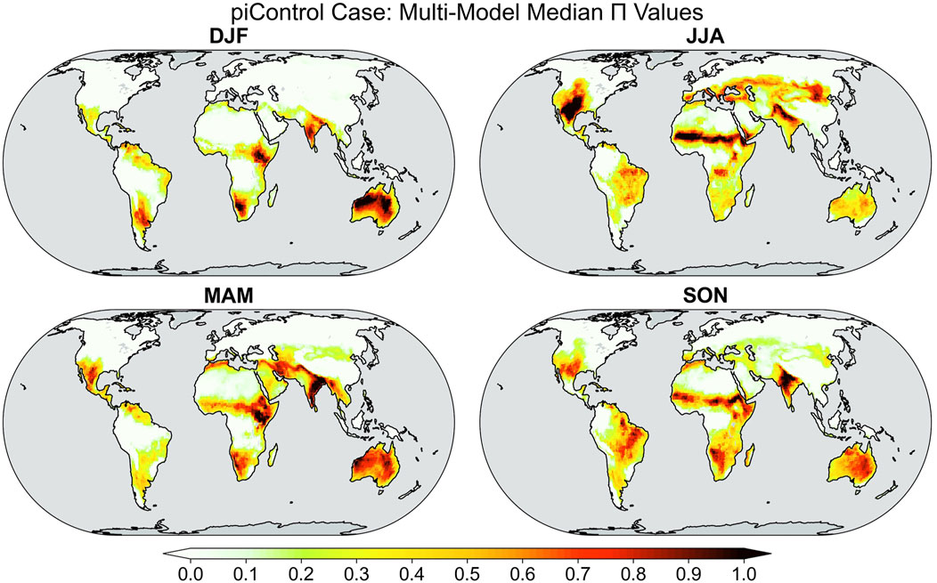
FIGURE 1. Multimodel median values of soil moisture–temperature coupling ($\Pi$; dimensionless) for each season from preindustrial control (piControl) simulations from CMIP6. Values are calculated over ice-free land areas only.

When comparing the coupling metric $\Pi$ from the late historical period relative to the piControl baseline (Figure 2), the median change is dominated by decreased soil moisture–temperature coupling across every season, with 99% confidence in the 30-model level of consensus. These areas of change largely correspond to regions of land cover change during the same interval, namely, the expansion of agriculture (North America, eastern Europe into central Asia, Northern China, and Northeast Brazil). Such differential effects of vegetation on extreme heat demonstrate the importance of biophysical indicators (Teuling et al., 2010). While some of the widespread areas of reduction over Africa appear to correspond to agricultural expansion, it is not indicated to be as widespread in the Hurtt et al. (2020) dataset as appears in Figure 2. Moreover, areas with indications of increasing $\Pi$ are small, scattered, and not greater than random chance in terms of field significance. Additionally, nearly one-third of the global land area displays increase in $\Pi$ across each season; however, when screening for significant model consensus, almost none of these areas pass the testing criterion.

FIGURE 2

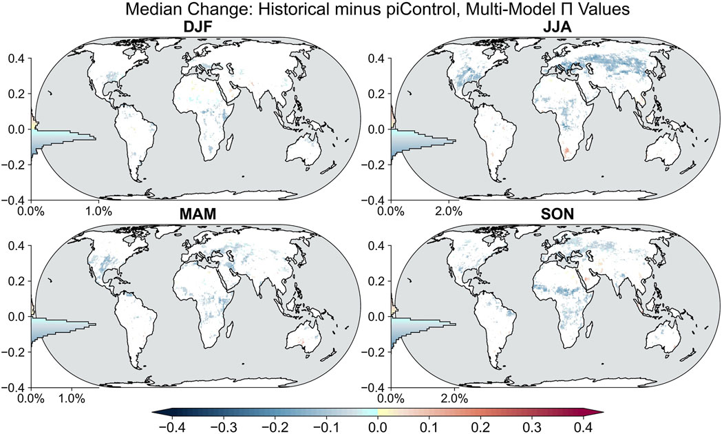
FIGURE 2. Multimodel median change in $\Pi$ (dimensionless) for each season from piControl to the last 50 years of the historical simulations in CMIP6. Areas are masked where the agreement among models on the sign of the change is below the 99% confidence level, or where the median of seasonal mean near-surface air temperature is below 0°C. Histograms show the probability distribution of significant changes as a fraction of the total land area.

As climate would be projected to approach the doubled CO₂ level with no other changes from piControl conditions (Figure 3), decreases in $\Pi$ again dominate in every season. Globally, two regions show most of this negative trend, one in Africa (mainly East Africa) and one in India. Both CMIP5 and CMIP6 models project wetter conditions over these regions (Zhao and Dai, 2015; Wang et al., 2020; Dosio et al., 2021; Zhao and Dai, 2022), and CMIP5 models had indicated reduced sensible heat flux over these areas (Dirmeyer et al., 2013b). A few contiguous areas show consensus seasonal increases in $\Pi$: the Western Mediterranean, Northern Indus and Ganges basins, the Southern Great Plains and northern Mexico during boreal winter, the South-central U.S., parts of Europe and central Australia during MAM, much of Europe and southern Arabia in SON, and just scattered and diffuse locations during JJA. Note that there is no land use change specified in this experiment, but most of these models predict vegetation phenology and about half include dynamic vegetation parameterizations.

FIGURE 3

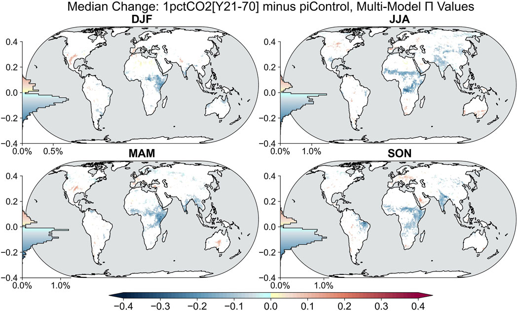
FIGURE 3. As in Figure 2 for the median change in $\Pi$ (dimensionless) from piControl to years 21–70 of the 1pctCO2 simulations (leading up to a doubling of CO₂).

Shifting to the quadrupling CO₂ scenario, the strongest and most widespread signals emerge. Areas of decreased soil moisture–temperature coupling in Africa and India persist and are joined by a large area of eastern South America during the JJA and SON seasons (Figure 4). However, there is a robust appearance of increased soil moisture control on extreme heat over many parts of the world across all seasons, matching or exceeding the area of decreased coupling. Beginning with boreal spring (MAM), a band of large consensus increases exists in $\Pi$ across much of the Mediterranean region from Spain to Turkey. Additionally, many broad areas of smaller consensus increases are indicated, spanning across central Asia and North America, from the central Great Plains westward across the central Rocky Mountains. Large areas over the western Sahara exhibit small consensus increases in $\Pi$. In the tropics, large fractions of Indonesia, the Amazon, and Congo basins show increases, while Southern Hemisphere subtropics across both continents display a scattering of increased $\Pi$ distribution.

FIGURE 4

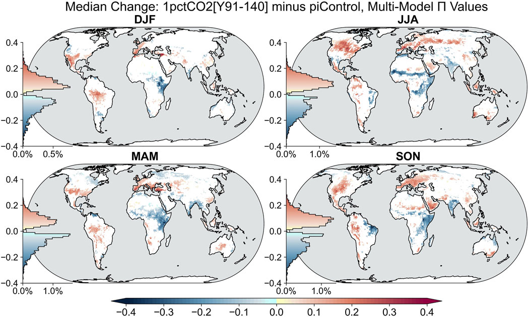
FIGURE 4. As in Figure 2 for the median change in $\Pi$ (dimensionless) from piControl to years 91–140 of the 1pctCO2 simulations (leading up to a quadrupling of CO₂).

Moving into boreal summer and austral winter, widespread areas of strong increases in $\Pi$ emerge. Over North America, there is a band over the entire Northern portion of the midlatitude agricultural belt, as well as portions of the Eastern U.S. and much of the North American monsoon region. Over Eurasia, there is a similar band of large changes stretching from Southern France to the Asian Taiga in Northern Kazakhstan across to Mongolia and northward into Finland. The small magnitude consensus increases over the desert shift to the Eastern Sahara, most of Arabia, and into Southern Iran. There are also small magnitude consensus increases over parts of Southeast Asia and China. In the tropics, there are large increases in $\Pi$ over the western parts of the Congo and Amazon Basins, the latter extending Northward into the Guianas. Areas in the Southern Hemisphere with Mediterranean climates (South Africa, Western Australia, and Chile) also have large increases, while Antarctica was masked from this investigation. Concomitantly, most of the Arctic displays little visible variability among coupling regimes across experiments, baseline climatology, and external forcing, that is, little variability is indicated based on the significance criterion (i.e., no positive statistical significance in soil moisture–heat coupling.)

In boreal fall and austral spring, broad areas of large increases persist in the Americas: over the central Rockies, Northern Great Plains, Northern Mexico, western Amazon, and Venezuela. Nearly all of Europe south of 55°N shows a consensus increase in $\Pi$, including the Caucasus region. There is also a band across Africa and Arabia north of 15°N and over southeastern Australia and South Africa. This season shows the greatest areal coverage of significant changes in the Arctic, mostly small decreases in land–heat coupling strength.

During boreal winter and austral summer (DJF), the most prominent feature is the broad area of a strong increase in $\Pi$ over most of Mexico and the southwestern U.S. A weaker but larger area is seen over much of South America between the equator and 20°S east of the Andes. In the Eastern Hemisphere, regions of consensus increase in $\Pi$ are patchy, with the areas of strongest increase over the Maghreb, the Levant, Tigris Basin, and upper Indus and Ganges basins. A sizeable fraction of southern Africa also shows consensus changes.

When compared to the median values of $\Pi$ from the piControl simulations, most of the consensus changes outside the low latitudes are poleward extensions of existing regions of strong soil moisture–temperature coupling, consistent with previous findings suggesting a poleward shift in land–atmosphere coupling regimes (Dirmeyer et al., 2013a; Dirmeyer et al., 2013b), for example, in the JJA panel of Figure 4, north of 30°N, changes where the piControl values of $\Pi$ are between 0.2 and 0.5 and average between + 0.02 and + 0.03, while above and below that range of $\Pi$, the mean changes are smaller. At low latitudes, areas of pronounced increases in $\Pi$ are also mainly an extension of higher values into regions that had low values in the piControl simulations and not an amplification of soil moisture–temperature coupling in a place where it is already strong.

3.2 Episodic coupling

Miralles et al. (2012) developed an instantaneous land–heat coupling metric $\left(\pi \right)$ that has been applied here to the CMIP6 model simulations at monthly timescales. The $\pi$ metric indicates the degree to which a specific episode of extreme heat is driven by a feedback chain from soil moisture and surface fluxes to air temperature. As demonstrated by Eq. 4, $\pi$ is based on differences and products of normalized anomalies, that is, standard normal deviates (Koster et al., 2009). There exists a quandary for statistics of this type when applied in a nonstationary climate, as notions of “anomaly” and “variance” are dependent on the definition of the mean, a definition representative of normal conditions. What means should be used? Should one base normality on the conditions before anthropogenic climate change began, or should it be defined more proximate to the point in time under consideration?

Conventionally, climate normals are defined using a trailing 30-year (or in common practice, a complete prior 3 decade) mean (Arguez and Vose, 2011), but it has been recognized that this practice is becoming inappropriate in a changing climate as the basis of defining anomalies for predicted events (e.g., Livezey et al., 2007; Milly et al., 2008). One alternative is to fit a regression, linear or otherwise, to data to create a time-varying normal. However, we should first ask the question of the purpose of a metric like $\pi$. It was conceived to be an indicator of the strength of a physical process, namely, the contribution of the land surface to the severity of heatwaves, and that is a quantity that is worthwhile to estimate for past and future as well as present climate conditions. We examine here if it is possible to use $\pi$ for this purpose, particularly how the definitions of the means ($\overline{T},\overline{H},\overline{H_p}$) used to calculate the anomalies ($T^{\prime },H^{\prime },H_p^{\prime }$) and the mean used as a baseline to calculate the standard deviations (${\sigma }_T$, ${\sigma }_H$, ${\sigma }_{H_p}$) affect $\pi$ and its interpretation.

Figure 5 shows the result for the preindustrial simulations (piControl)—it is to be noted that the scale for $\pi$ is different compared to that for $\Pi$. Large values suggest regions where there is a stronger land surface feedback on extreme heat. In austral summer (DJF), Northern Australia, inland Southern Africa, and South America, and the Amazon delta have some of the highest values. In MAM, there is a northward shift, with the strongest feedbacks indicated over a smaller portion of Northern Australia, Southeast Asia, from the Guinea coast of Africa eastward to the Ethiopian Highlands, and small areas on the continents around the Caribbean Sea and the Gulf of Mexico. By JJA, large contiguous areas of large $\pi$ emerge over much of southern North America and the Sahel region of Africa, along with scattered smaller areas, such as over Northwestern India. During SON, much of tropical and subtropical South America shows very high values, as well as several areas scattered across East Africa.

FIGURE 5

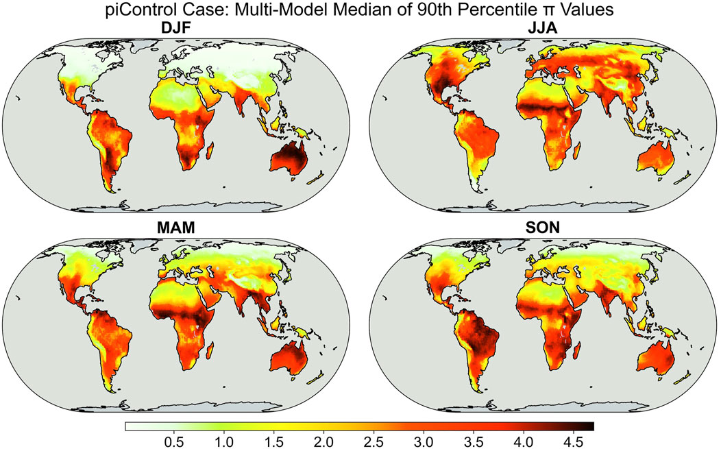
FIGURE 5. Multimodel median of the 90th percentile values of monthly scale soil moisture–temperature coupling ($\pi$; dimensionless) for each season from preindustrial control (piControl) simulations. Values are calculated over ice-free land areas only.

Regionally, there are some clear patterns of seasonality. North America and much of midlatitude Eurasia show a clear oscillation between summer and winter. In East Asia, there is a South-to-North progression of high $\pi$ values into summer but also an outbreak from a hotspot around Beijing and the Gobi Desert in MAM that expands across the Eurasian Steppes by JJA. However, regions like Mexico and India appear to maintain strong land surface feedbacks to heatwaves throughout the year, as does most of sub-Saharan Africa. Nearly all land in the Southern Hemisphere is covered in shades of red throughout the year, as shown in Figure 5.

High values of $\pi$ correspond quite well with the seasons and locations of so-called hotspots of land–atmosphere coupling (e.g., Koster et al., 2004; Dirmeyer et al., 2009). Low values of $\pi$ do not indicate a lack of heat or heatwaves but rather a lack of land surface contribution via concomitant soil drying. It is to be noted that the large deserts of Africa and Asia in Figure 5 usually have low values of the 90th percentile of $\pi$. Cool and/or moist regions also have low values for the 90th percentile of $\pi$ as they rarely, if ever, get into a state of concurrent dry soils and prolonged extreme heat.

We can see the impact of our choice of baseline for the definition of anomalies when we examine changes in the 90th percentile of $\pi$ from the preindustrial to recent historical times (Figure 6 depicts JJA; other seasons are shown in Supplementary Figure S2). When each period’s anomalies and standard deviations for temperature, sensible heat, and potential sensible heat are used for each model, the left panel shows that the multimodel median of the 90th percentile value of $\pi$ shows a significant consensus change over portions of the globe. Decreases correspond largely to areas of land cover change: areas of agricultural expansion over the Americas, Northeast China, India, the Sahel, and Australia, but the correspondence between land use change and land-heat coupling has not been explicitly quantified in this study as it has been in others (e.g., Chen and Dirmeyer, 2019; Chen and Dirmeyer, 2020; Hu and Sun, 2022). Increases are largely confined to low latitudes, corresponding to areas of tropical deforestation but also in the subtropics of the Southern Hemisphere during austral summer (Figure 2) and, curiously, much of the Sahara. The multimodel median values of the time mean and standard deviations that are part of the main terms in $\pi$ (Eq. 4) are shown for all seasons in Supplementary Figures S3, S4, respectively.

FIGURE 6

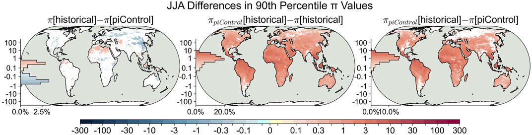
FIGURE 6. JJA multimodel median of differences in the 90th percentile values of $\pi$ (dimensionless). The left map shows differences when $\pi$ is calculated from the last 50 years’ data from the historical simulations and $\pi$ from piControl. The middle map shows the difference when means and standard deviations from the piControl climatology are used to calculate $\pi$ for the late historical period versus using all climate statistics from the historical period. The right map shows the change from piControl to the late historical period when piControl climatology is used as the basis for calculating $\pi$ in both periods. Areas are masked where the agreement among models on the sign of the change is below the 99% confidence level, or where the median of seasonal mean near-surface air temperature is below 0°C. Histograms show the probability distribution of significant changes as a fraction of the total land area.

This pattern of change in the 90th percentile of $\pi$ is driven by several factors. Most areas experienced warming (Supplementary Figure S5). There is an increase in the standard deviation of temperature almost everywhere (Supplementary Figure S6), which makes the denominator larger for the historical case. Notable exceptions, according to the models, include areas with large increases in cultivation: central North America, Far East Asia, the upper Ganges and Indus valleys, and much of Eastern Europe. The mean and standard deviation of sensible heat flux drop over most of the same areas. The changes in potential sensible heat closely mirror temperature changes over the Western Hemisphere but not in the Eastern Hemisphere. As a global measure of the drivers of changes in $\pi$, we calculated spatial correlations of its changes in each season (from Figure 6 andSupplementary Figure S2) with the changes in each time-mean term in Eq. 4. Changes in ${\sigma }_T$ explain 79% of the spatial variance during MAM and JJA, 71% in SON, and 55% in DJF. ${\sigma }_H$ and ${\sigma }_{H_p}$ also explain around 50% of the variance on average and as much as 62% in MAM (note that these terms are cross-correlated; therefore, percentages for any season can sum to more than 100%). Changes in the means $\overline{T}$, $\overline{H}$, and $\overline{H_p}$ generally account for less than 30% of the variance.

Returning to Figure 6, we see a very different picture when the baseline for anomalies during the historical period is kept at piControl levels and the piControl standard deviations for the terms used to calculate $\pi$ are also used (right panel). Nearly every significant change is a substantial increase, suggesting stronger land surface coupling to extreme heat events. The middle panel of Figure 6 shows the difference that arises mainly from the differing estimates of the 90th percentile of $\pi$ during the historical period between the two baselines.

Next, we examine the doubled and quadrupled CO₂ periods compared with piControl. Using a trailing 30-year mean as the basis for climatology in the future projections, we see a pattern of changes for the quadrupled CO₂ case (Figure 7) that is very similar to but skewed more strongly to positive differences and more significant areal coverage than the doubled CO₂ case (Supplementary Figure S7). During all seasons, there are widespread consensus increases in the 90th percentile of $\pi$, the largest of which locally amounts to 20%–40% increases over piControl coupling strengths. Areas of consistent exception are around the Mediterranean and North Africa, as well as South Africa, indicating weaker coupling of soil moisture to extreme heat in most seasons. During boreal summer, the areas of decreased $\pi$ expand to their greatest area in several subtropical regions and some hot midlatitude locations in the Northern Hemisphere. The broad expanse of stronger land feedbacks to heat across the entire Arctic as well as across much of the tropics is striking. During SON, there are only a few areas of decrease in the Southern Hemisphere. DJF shows Australia to be exempted from increased soil moisture feedbacks on extreme heat, along with Namibia, the Maghreb, and the Pampas.

FIGURE 7

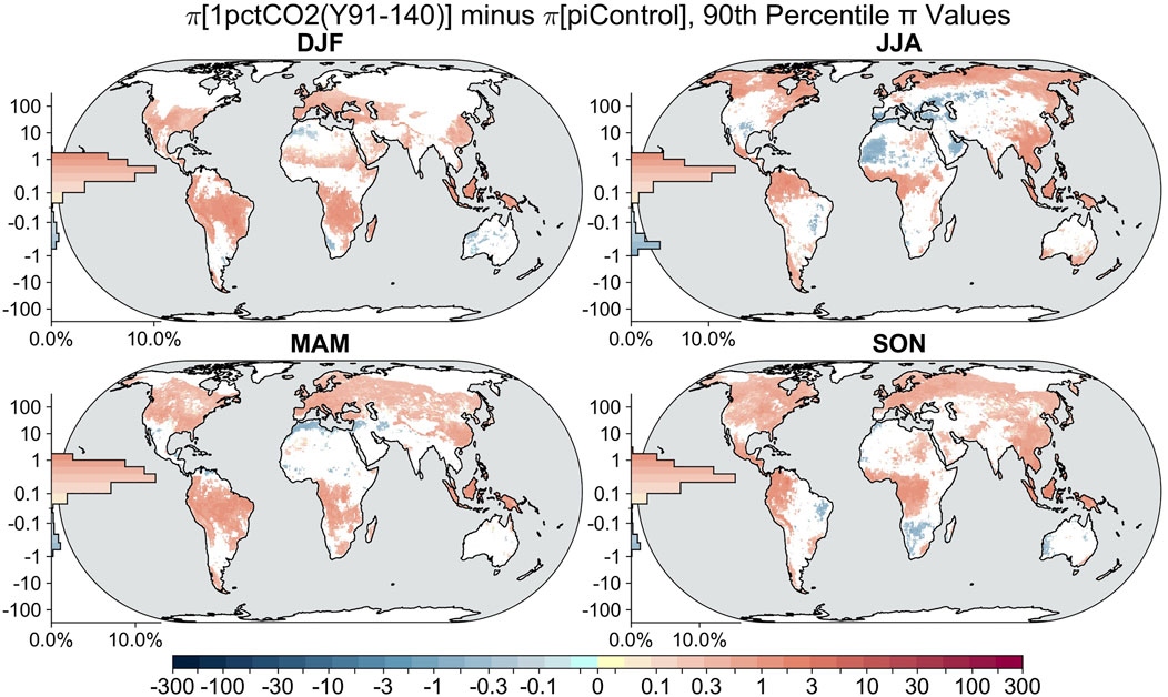
FIGURE 7. Multimodel median of differences in the 90th percentile values of $\pi$ (dimensionless) for the period of 1pctCO2 approaching quadrupled CO₂ minus piControl for each season. Areas are masked where the agreement among models on the sign of the change is below the 99% confidence level, or where the median of seasonal mean near-surface air temperature is below 0°C. Histograms show the probability distribution of significant changes as a fraction of the total land area.

Unsurprisingly, if the preindustrial norms are used as the basis for calculating $\pi$ in future climate scenarios, the values become huge because the anomalies are huge. We have examined several variants–one of the most instructive is to calculate anomalies for future climate scenarios based on the trailing 30-year means in those cases but to retain the standard deviations from piControl when normalizing the terms in $\pi$. This seems reasonable since there is likely to be some degree of adjustment by populations and migrating ecosystems to increasing temperatures, but changes in variability may not be easily accommodated. Figure 8 shows the difference in the 90th percentile of $\pi$ for each season in this case compared to the maps shown in Figure 7 (Supplementary Figure S8 is the equivalent for the doubled CO₂ case). When the three factors in $\pi$ are normalized by piControl standard deviations, rather than future standard deviations, stronger land feedbacks on extreme heat are indicated across the tropics and subtropics. The area skews toward the summer hemisphere as seasons progress, showing that the added impacts are mainly in monsoonal areas. However, arid regions and seasons in the subtropics and tropics experience less land feedback on heat in this formulation. Means and standard deviations of temperature will increase globally in all seasons in the future (Supplementary Figures S9–S12), but the areas showing a reduction in the 90th percentile of $\pi$ shown in Figure 8 correspond with regions of decreased variability in potential sensible heat flux (and thus potential evaporation), while the areas of increase align well with areas of increased sensible heat flux variability. Changes in ${\sigma }_T$ again explain most of the spatial variance, generally more than 80% for both future scenarios. ${\sigma }_H$ and ${\sigma }_{H_p}$ explain a comparable amount for quadrupled CO₂ as they did for the historical changes but slightly less for doubled CO₂. Changes in the mean terms account for about a quarter of the spatial variance.

FIGURE 8

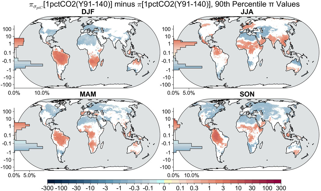
FIGURE 8. As in Figure 7 but with future values of $\pi$ (dimensionless) based on means and standard deviations from the piControl climatology.

4 Discussion and conclusion

This study estimates past, present, and future heatwave susceptibility based on surface temperature, surface sensible heat flux, and surface latent heat flux as proposed by Miralles et al. (2012). The impact of climate change on climatological coupling via land–atmosphere temperature feedbacks has been examined with the climatological metric $\left(\Pi \right)$ from Miralles et al. (2012). This metric considers differing correlations between near-surface air temperature relative to potential and sensible heat flux, the former equivalent to the difference between net radiation and potential latent heat flux. Furthermore, this coupling can be robustly investigated, as it is based on temporal correlations that can well reflect changing relationships among physical climate variables such as temperature and sensible heat. This is more broadly true for correlation-based investigations of other evolving biotic indicators and land–atmosphere feedbacks in a changing climate (e.g., Notaro, 2008; Dirmeyer et al., 2013b; Berg et al., 2015; Lorenz et al., 2015; Santanello et al., 2018; Schwingshackl et al., 2018). However, the connection between these variables may not be strictly linear but can change depending on the role of soil moisture in modulating surface heat fluxes (Benson and Dirmeyer, 2021; Dirmeyer et al., 2021). It remains to be shown whether there is a better land-heat metric to use with CMIP6 model data.

Under preindustrial conditions (piControl), seasonally dependent hotspot regions of land–atmosphere coupling typically located in transitional zones between wet and dry climates in many other studies emerge once more during this analysis for $\Pi$ (Figure 1). Among CMIP6 models, historical land-use change (e.g., agriculture) corresponds spatially to areas of reduced land surface (i.e., soil moisture) controls on extreme heat (Figure 2). This relationship is consistent with crops’ lack of regulation of their evapotranspiration as they have been bred to produce ample fruit rather than to survive extremes. Moreover, land surface models reflect these trade-off features via increases in gross primary productivity, high stomatal conductance, and vigorous carbon assimilation (De Kauwe et al., 2015; Franks et al., 2018).

For the future climate scenarios (Figures 3, 4), coverage of increased soil moisture–heat flux–temperature coupling (i.e., positive values of $\Pi$) emerges as doubled atmospheric CO₂ is approached, while regions displaying a reduction in land–atmosphere coupling early in the 1pctCO2 simulations begin to recede over time during every season. As quadrupled CO₂ is approached, regions of increasing land-heat coupling begin to dominate, particularly in monsoonal areas and across much of the midlatitudes where areas of seasonally high values of $\Pi$ spread northward.

Consideration of the episodic land–atmosphere heat coupling metric of Miralles et al. (2012), $\pi$, focuses on changes of its 90th percentile value in each season, including “cold” seasons that might not be considered as having heatwaves. This is done for completeness, as arbitrarily excluding months is difficult to justify. The low-temperature screening described at the end of Section 2 is our attempt to remove severely energy-limited situations from consideration. All seasons have been considered because episodes of extreme heat are not only intensifying (and projected to intensify further, cf. Perkins-Kirkpatrick and Gibson, 2017) but are also spreading in many places into seasons not historically associated with heatwaves (Shafiei Shiva et al., 2019). Changes are shown globally for each season, compared to the preindustrial baseline.

It is a much more nuanced problem to attribute the role of the land surface in the proliferation of extreme events within a changing climate as the very definition of “extreme” is by nature relative and potentially changing. This is particularly true when metrics are built with the assumption of a stationary climate as opposed to a changing one (Milly et al., 2008; Trenberth et al., 2014; Stevenson et al., 2022). The metric $\pi$ falls into this category (Figure 5), as it is based on the normalization of anomalies with temporal standard deviations, each of which can be defined from different baselines. Anomalies have been defined based on a mean climate period, a trailing 30-year mean climatology, and relative to piControl in the presence of changing climate. Relative to piControl norms, 90th percentile indices of monthly land–atmosphere coupling increase significantly over the entire globe, especially for the most recent historical period (Figure 6 and Supplementary Figure S2), and they can grow to dozens of times more than the values when contemporaneous climate norms are used in the quadrupled CO₂ period (not shown). This throws into question the very meaning of such a metric.

Instead, two reasonable approaches are explored. When contemporaneous climate means and standard deviations (i.e., based on the trailing 30 years) are used to compare different periods (Figure 7 and Supplementary Figure S7), increased coupling from land to extreme heat cases becomes widespread over the moist tropics, much of the extratropics, and especially during summer in high-latitude regions. Decreased coupling appears over some of the more arid regions. However, one may assume that gradually increasing mean temperatures are not as much a factor for assessing land–atmosphere feedbacks as the changes in variability. When piControl standard deviations of temperature, sensible heat flux, and normalized sensible heat flux are used in all time periods, but anomalies are calculated based on recent climate norms, a different picture emerges (Figure 8 and Supplementary Figure S8). Increases in the 90th percentile of $\pi$ become quite large across the tropics and monsoon regions as well as northern Europe during the boreal summer, reflecting an increase in surface heat flux variability across the region in tandem with increasing temperature variability (Supplementary Figures S10, S12). Other regions mostly indicate a reduction in heat flux variability relative to piControl norms, suggesting that the land surface is less involved in the development of temperature extremes.

These conclusions should be considered provisional and serve mainly as an indicator of the difficulty surrounding the construction of an interdisciplinary, widely applicable metric, that is, navigating through the uncertainty presented by a changing climate and the Earth system processes fostering these extreme events. For modeling studies, it is rather difficult to isolate and deduce a posteriori the role of land surface feedbacks on extremes (e.g., heatwaves and drought) from experiments that were not specifically designed to isolate the possible role of the land via specifically constructed sensitivity analyses. This discontinuity points to the merit and necessity of targeted multimodel climate change experiments (Seneviratne et al., 2013; Hurk et al., 2016; Lawrence et al., 2016). However, with an abundance of subfield-specific model intercomparison projects (MIPs; over 20 in CMIP6), such specialized sensitivity studies become undersubscribed and model uncertainty is amplified.

Projects like GSWP-2 (Dirmeyer et al., 2006), GLACE (Koster et al., 2004; Koster et al., 2006), GLACE-2 (Koster et al., 2011), and LUCID (Pitman et al., 2009) established a model count of about one dozen as an adequate minimum for global climate studies–a mark that has been difficult to match with recent specialized MIPs. However, these innovative strategies must progress beyond the monthly scale analyses presented here in addition to investigating changes in actual heatwave events that would require daily model output. Such data are available for a few CMIP6 models, but the sample distribution is not large enough to assuage concerns over model-dependent results. Furthermore, the relatively low resolution of climate change models may obscure processes and localized features that could alter these results. Perhaps for the next round of climate model intercomparisons, MIPs can be organized that target phenomena of looming societal concern such as heatwaves and droughts.

Data availability statement

The original contributions presented in the study are included in the article/Supplementary Material; further inquiries can be directed to the corresponding author.

Author contributions

PD conceived of the original research project and led the analysis and writing. RM and PD conducted data processing and computations. BG organized the discussion of the analysis and drafted the manuscript. DK, BG, RM, and PD contributed to the analysis of results and the manuscript.

Funding

PD’s participation was supported by National Oceanographic and Atmospheric Administration grant NA20OAR4310422. RM’s participation was supported by National Oceanographic and Atmospheric Administration grant NA20OAR4590316. BG’s participation was supported by the Department of Geography and Geoinformation Science at George Mason University. Data processing and preliminary analyses for this study were performed by the coauthors as part of a graduate class project in land–climate interactions in the Climate Dynamics Program of George Mason University, Fairfax, Virginia, United States. The lead author’s synthesis of the student material was supported by the Center for Ocean Land Atmosphere Studies (COLA).

Acknowledgments

The authors acknowledge Zahra Ghodsi Zadeh and Geoffrey Rath for their early participation in this work. Additionally, the authors thank Dr. René Orth and two reviewers for their constructive comments that have substantially improved the study and the effort of one reviewer to provide the collated list of specific atmosphere and land model component information in Supplementary Table S1, which saved us a great deal of effort.

Conflict of interest

The authors declare that the research was conducted in the absence of any commercial or financial relationships that could be construed as a potential conflict of interest.

Publisher’s note

All claims expressed in this article are solely those of the authors and do not necessarily represent those of their affiliated organizations, or those of the publisher, the editors, and the reviewers. Any product that may be evaluated in this article, or claim that may be made by its manufacturer, is not guaranteed or endorsed by the publisher.

Supplementary material

The Supplementary Material for this article can be found online at: https://www.frontiersin.org/articles/10.3389/fenvs.2022.949250/full#supplementary-material

References

Abramowitz, G., Herger, N., Gutmann, E., Hammerling, D., Knutti, R., Leduc, M., et al. (2019). ESD reviews: Model dependence in multi-model climate ensembles: Weighting, sub-selection and out-of-sample testing. Earth Syst. Dyn. 10, 91–105. doi:10.5194/esd-10-91-2019

CrossRef Full Text | Google Scholar

Albergel, C., Dutra, E., Bonan, B., Zheng, Y., Munier, S., Balsamo, G., et al. (2019). Monitoring and forecasting the impact of the 2018 summer heatwave on vegetation. Remote Sens. 11, 520. doi:10.3390/rs11050520

CrossRef Full Text | Google Scholar

Arguez, A., and Vose, R. S. (2011). The definition of the standard WMO climate normal: The key to deriving alternative climate normals. Bull. Am. Meteorol. Soc. 92, 699–704. doi:10.1175/2010BAMS2955.1

CrossRef Full Text | Google Scholar

Benson, D. O., and Dirmeyer, P. A. (2021). Characterizing the relationship between temperature and soil moisture extremes and their role in the exacerbation of heat waves over the contiguous United States. J. Clim. 34, 2175–2187. doi:10.1175/JCLI-D-20-0440.1

CrossRef Full Text | Google Scholar

Berg, A., Lintner, B. R., Findell, K., Seneviratne, S. I., Hurk, B., Ducharne, A., et al. (2015). Interannual coupling between summertime surface temperature and precipitation over land: Processes and implications for climate change. J. Clim. 28, 1308–1328. doi:10.1175/JCLI-D-14-00324.1

CrossRef Full Text | Google Scholar

Bevacqua, E., Zappa, G., Lehner, F., and Zscheischler, J. (2022). Precipitation trends determine future occurrences of compound hot–dry events. Nat. Clim. Chang. 12, 350–355. doi:10.1038/s41558-022-01309-5

CrossRef Full Text | Google Scholar

Brunner, L., Pendergrass, A. G., Lehner, F., Merrifield, A. L., Lorenz, R., and Knutti, R. (2020). Reduced global warming from CMIP6 projections when weighting models by performance and independence. Earth Syst. Dyn. 11, 995–1012. doi:10.5194/esd-11-995-2020

CrossRef Full Text | Google Scholar

Chen, L., and Dirmeyer, P. A. (2019). The relative importance among anthropogenic forcings of land use/land cover change in affecting temperature extremes. Clim. Dyn. 52, 2269–2285. doi:10.1007/s00382-018-4250-z

CrossRef Full Text | Google Scholar

Chen, L., and Dirmeyer, P. A. (2020). Distinct impacts of land use and land management on summer temperatures. Front. Earth Sci. (Lausanne). 8, 245. doi:10.3389/feart.2020.00245

CrossRef Full Text | Google Scholar

De Kauwe, M. G., Kala, J., Lin, Y.-S., Pitman, A. J., Medlyn, B. E., Duursma, R. A., et al. (2015). A test of an optimal stomatal conductance scheme within the CABLE land surface model. Geosci. Model Dev. 8, 431–452. doi:10.5194/gmd-8-431-2015

CrossRef Full Text | Google Scholar

Dee, D. P., Uppala, S. M., Simmons, A. J., Berrisford, P., Poli, P., Kobayashi, S., et al. (2011). The ERA-interim reanalysis: Configuration and performance of the data assimilation system. Q. J. R. Meteorol. Soc. 137, 553–597. doi:10.1002/qj.828

CrossRef Full Text | Google Scholar

Dirmeyer, P. A., Balsamo, G., Blyth, E. M., Morrison, R., and Cooper, H. M. (2021). Land-atmosphere interactions exacerbated the drought and heatwave over northern Europe during summer 2018. AGU Adv. 2, e2020AV000283. doi:10.1029/2020AV000283

CrossRef Full Text | Google Scholar

Dirmeyer, P. A., Gao, X., Zhao, M., Guo, Z., Oki, T., and Hanasaki, N. (2006). GSWP-2: Multimodel analysis and implications for our perception of the land surface. Bull. Am. Meteorol. Soc. 87, 1381–1398. doi:10.1175/BAMS-87-10-1381

CrossRef Full Text | Google Scholar

Dirmeyer, P. A., Jin, Y., Singh, B., and Yan, X. (2013a). Evolving land–atmosphere interactions over north America from CMIP5 simulations. J. Clim. 26, 7313–7327. doi:10.1175/JCLI-D-12-00454.1

CrossRef Full Text | Google Scholar

Dirmeyer, P. A., Jin, Y., Singh, B., and Yan, X. (2013b). Trends in land–atmosphere interactions from CMIP5 simulations. J. Hydrometeorol. 14, 829–849. doi:10.1175/JHM-D-12-0107.1

CrossRef Full Text | Google Scholar

Dirmeyer, P. A., Schlosser, C. A., and Brubaker, K. L. (2009). Precipitation, recycling, and land memory: An integrated analysis. J. Hydrometeorol. 10, 278–288. doi:10.1175/2008JHM1016.1

CrossRef Full Text | Google Scholar

Dirmeyer, P. A. (2011). The terrestrial segment of soil moisture-climate coupling. Geophys. Res. Lett. 38, L16702. doi:10.1029/2011GL048268

CrossRef Full Text | Google Scholar

Dosio, A., Jury, M. W., Almazroui, M., Ashfaq, M., Diallo, I., Engelbrecht, F. A., et al. (2021). Projected future daily characteristics of African precipitation based on global (CMIP5, CMIP6) and regional (CORDEX, CORDEX-CORE) climate models. Clim. Dyn. 57, 3135–3158. doi:10.1007/s00382-021-05859-w

CrossRef Full Text | Google Scholar

Eyring, V., Bony, S., Meehl, G. A., Senior, C. A., Stevens, B., Stouffer, R. J., et al. (2016). Overview of the coupled model intercomparison project Phase 6 (CMIP6) experimental design and organization. Geosci. Model Dev. 9, 1937–1958. doi:10.5194/gmd-9-1937-2016

CrossRef Full Text | Google Scholar

Fischer, E. M., Seneviratne, S. I., Lüthi, D., and Schär, C. (2007). Contribution of land-atmosphere coupling to recent European summer heat waves. Geophys. Res. Lett. 34, L06707. doi:10.1029/2006GL029068

CrossRef Full Text | Google Scholar

Franks, P. J., Bonan, G. B., Berry, J. A., Lombardozzi, D. L., Holbrook, N. M., Herold, N., et al. (2018). Comparing optimal and empirical stomatal conductance models for application in Earth system models. Glob. Chang. Biol. 24, 5708–5723. doi:10.1111/gcb.14445

PubMed Abstract | CrossRef Full Text | Google Scholar

Hauser, M., Orth, R., and Seneviratne, S. I. (2016). Role of soil moisture versus recent climate change for the 2010 heat wave in Western Russia. Geophys. Res. Lett. 43, 2819–2826. doi:10.1002/2016GL068036

CrossRef Full Text | Google Scholar

Hirsch, A. L., Evans, J. P., Virgilio, G. D., Perkins‐Kirkpatrick, S. E., Argüeso, D., Pitman, A. J., et al. (2019). Amplification of Australian heatwaves via local land-atmosphere coupling. J. Geophys. Res. Atmos. 124, 13625–13647. doi:10.1029/2019JD030665

CrossRef Full Text | Google Scholar

Hu, T., and Sun, Y. (2022). Anthropogenic influence on extreme temperatures in China based on CMIP6 models. Int. J. Climatol. 42, 2981–2995. doi:10.1002/joc.7402

CrossRef Full Text | Google Scholar

Hurk, B., Kim, H., Krinner, G., Seneviratne, S. I., Derksen, C., Oki, T., et al. (2016). LS3MIP (v1.0) contribution to CMIP6: The land surface, snow and soil moisture model intercomparison project – aims, setup and expected outcome. Geosci. Model Dev. 9, 2809–2832. doi:10.5194/gmd-9-2809-2016

CrossRef Full Text | Google Scholar

Hurtt, G. C., Chini, L., Sahajpal, R., Frolking, S., Bodirsky, B. L., Calvin, K., et al. (2020). Harmonization of global land use change and management for the period 850–2100 (LUH2) for CMIP6. Geosci. Model Dev. 13, 5425–5464. doi:10.5194/gmd-13-5425-2020

CrossRef Full Text | Google Scholar

Knutti, R., Furrer, R., Tebaldi, C., Cermak, J., and Meehl, G. A. (2010). Challenges in combining projections from multiple climate models. J. Clim. 23, 2739–2758. doi:10.1175/2009JCLI3361.1

CrossRef Full Text | Google Scholar

Koster, R. D., Dirmeyer, P. A., Guo, Z., Bonan, G., Chan, E., Cox, P., et al. (2004). Regions of strong coupling between soil moisture and precipitation. Science 305, 1138–1140. doi:10.1126/science.1100217

PubMed Abstract | CrossRef Full Text | Google Scholar

Koster, R. D., Sud, Y. C., Guo, Z., Dirmeyer, P. A., Bonan, G., Oleson, K. W., et al. (2006). Glace: The global land–atmosphere coupling experiment. Part I: Overview. J. Hydrometeorol. 7, 590–610. doi:10.1175/JHM510.1

CrossRef Full Text | Google Scholar

Koster, R. D., Guo, Z., Yang, R., Dirmeyer, P. A., Mitchell, K., and Puma, M. J. (2009). On the nature of soil moisture in land surface models. J. Clim. 22, 4322–4335. doi:10.1175/2009JCLI2832.1

CrossRef Full Text | Google Scholar

Koster, R. D., Mahanama, S. P. P., Yamada, T. J., Balsamo, G., Berg, A. A., Boisserie, M., et al. (2011). The second Phase of the global land–atmosphere coupling experiment: Soil moisture contributions to subseasonal forecast skill. J. Hydrometeorol. 12, 805–822. doi:10.1175/2011JHM1365.1

CrossRef Full Text | Google Scholar

Krishnamurti, T. N., Kishtawal, C. M., LaRow, T. E., Bachiochi, D. R., Zhang, Z., Williford, C. E., et al. (1999). Improved weather and seasonal climate forecasts from multimodel superensemble. Science 285, 1548–1550. doi:10.1126/science.285.5433.1548

PubMed Abstract | CrossRef Full Text | Google Scholar

Lau, N.-C., and Nath, M. J. (2014). Model simulation and projection of European heat waves in present-day and future climates. J. Clim. 27, 3713–3730. doi:10.1175/JCLI-D-13-00284.1

CrossRef Full Text | Google Scholar

Lawrence, D. M., Hurtt, G. C., Arneth, A., Brovkin, V., Calvin, K. V., Jones, A. D., et al. (2016). The land use model intercomparison project (LUMIP) contribution to CMIP6: Rationale and experimental design. Geosci. Model Dev. 9, 2973–2998. doi:10.5194/gmd-9-2973-2016

CrossRef Full Text | Google Scholar

Leduc, M., Laprise, R., Elía, R., and Šeparović, L. (2016). Is institutional democracy a good proxy for model independence? J. Clim. 29, 8301–8316. doi:10.1175/JCLI-D-15-0761.1

CrossRef Full Text | Google Scholar

Livezey, R. E., Vinnikov, K. Y., Timofeyeva, M. M., Tinker, R., and Dool, H. M. (2007). Estimation and extrapolation of climate normals and climatic trends. J. Appl. Meteorol. Climatol. 46, 1759–1776. doi:10.1175/2007JAMC1666.1

CrossRef Full Text | Google Scholar

Lorenz, R., Pitman, A. J., Hirsch, A. L., and Srbinovsky, J. (2015). Intraseasonal versus interannual measures of land–atmosphere coupling strength in a global climate model: GLACE-1 versus GLACE-CMIP5 experiments in ACCESS1.3b. J. Hydrometeorol. 16, 2276–2295. doi:10.1175/JHM-D-14-0206.1

CrossRef Full Text | Google Scholar

Martens, B., Miralles, D. G., Lievens, H., van der Schalie, R., de Jeu, R. A. M., Fernández-Prieto, D., et al. (2017). GLEAM v3: Satellite-based land evaporation and root-zone soil moisture. Geosci. Model Dev. 10, 1903–1925. doi:10.5194/gmd-10-1903-2017

CrossRef Full Text | Google Scholar

Milly, P. C. D., Betancourt, J., Falkenmark, M., Hirsch, R. M., Kundzewicz, Z. W., Lettenmaier, D. P., et al. (2008). Stationarity is dead: Whither water management? Science 319, 573–574. doi:10.1126/science.1151915

PubMed Abstract | CrossRef Full Text | Google Scholar

Miralles, D. G., Gentine, P., Seneviratne, S. I., and Teuling, A. J. (2019). Land–atmospheric feedbacks during droughts and heatwaves: State of the science and current challenges. Ann. N. Y. Acad. Sci. 1436, 19–35. doi:10.1111/nyas.13912

PubMed Abstract | CrossRef Full Text | Google Scholar

Miralles, D. G., van den Berg, M. J., Teuling, A. J., and de Jeu, R. A. M. (2012). Soil moisture-temperature coupling: A multiscale observational analysis. Geophys. Res. Lett. 39, L21707. doi:10.1029/2012GL053703

CrossRef Full Text | Google Scholar

Neal, E., Huang, C. S. Y., and Nakamura, N. (2022). The 2021 pacific northwest heat wave and associated blocking: Meteorology and the role of an upstream cyclone as a diabatic source of wave activity. Geophys. Res. Lett. 49, e2021GL097699. doi:10.1029/2021GL097699

CrossRef Full Text | Google Scholar

Notaro, M. (2008). Statistical identification of global hot spots in soil moisture feedbacks among IPCC AR4 models. J. Geophys. Res. 113, D09101. doi:10.1029/2007JD009199

CrossRef Full Text | Google Scholar

O, S., Bastos, A., Reichstein, M., Li, W., Denissen, J., Graefen, H., et al. (2022). The role of climate and vegetation in regulating drought-heat extremes. J. Clim. 1, 5677–5685. doi:10.1175/JCLI-D-21-0675.1

CrossRef Full Text | Google Scholar

Palmer, T. N., Alessandri, A., Andersen, U., Cantelaube, P., Davey, M., Délécluse, P., et al. (2004). Development of a EUROPEAN multimodel ensemble system for seasonal-to-interannual prediction (demeter). Bull. Am. Meteorol. Soc. 85, 853–872. doi:10.1175/BAMS-85-6-853

CrossRef Full Text | Google Scholar

Parker, W. S. (2013). Ensemble modeling, uncertainty and robust predictions. WIREs Clim. Change 4, 213–223. doi:10.1002/wcc.220

CrossRef Full Text | Google Scholar

Perkins-Kirkpatrick, S. E., and Gibson, P. B. (2017). Changes in regional heatwave characteristics as a function of increasing global temperature. Sci. Rep. 7, 12256. doi:10.1038/s41598-017-12520-2

PubMed Abstract | CrossRef Full Text | Google Scholar

Petch, J. C., Short, C. J., Best, M. J., McCarthy, M., Lewis, H. W., Vosper, S. B., et al. (2020). Sensitivity of the 2018 UK summer heatwave to local sea temperatures and soil moisture. Atmos. Sci. Lett. 21, e948. doi:10.1002/asl.948

CrossRef Full Text | Google Scholar

Pirtle, Z., Meyer, R., and Hamilton, A. (2010). What does it mean when climate models agree? A case for assessing independence among general circulation models. Environ. Sci. Policy 13, 351–361. doi:10.1016/j.envsci.2010.04.004

CrossRef Full Text | Google Scholar

Pitman, A. J., de Noblet-Ducoudré, N., Cruz, F. T., Davin, E. L., Bonan, G. B., Brovkin, V., et al. (2009). Uncertainties in climate responses to past land cover change: First results from the LUCID intercomparison study. Geophys. Res. Lett. 36, L14814. doi:10.1029/2009GL039076

CrossRef Full Text | Google Scholar

Priestley, C. H. B., and Taylor, R. J. (1972). On the assessment of surface heat flux and evaporation using large-scale parameters. Mon. Wea. Rev. 100, 81–92. doi:10.1175/1520-0493(1972)100<0081:OTAOSH>2.3.CO;2

CrossRef Full Text | Google Scholar

Samaniego, L., Thober, S., Kumar, R., Wanders, N., Rakovec, O., Pan, M., et al. (2018). Anthropogenic warming exacerbates European soil moisture droughts. Nat. Clim. Chang. 8, 421–426. doi:10.1038/s41558-018-0138-5

CrossRef Full Text | Google Scholar

Santanello, J. A., Dirmeyer, P. A., Ferguson, C. R., Findell, K. L., Tawfik, A. B., Berg, A., et al. (2018). Land-atmosphere interactions: The LoCo perspective. Bull. Am. Meteorol. Soc. 99, 1253–1272. doi:10.1175/BAMS-D-17-0001.1

CrossRef Full Text | Google Scholar

Schumacher, D. L., Keune, J., Heerwaarden, C. C., Arellano, J. V.-G., Teuling, A. J., and Miralles, D. G. (2019). Amplification of mega-heatwaves through heat torrents fuelled by upwind drought. Nat. Geosci. 12, 712–717. doi:10.1038/s41561-019-0431-6

CrossRef Full Text | Google Scholar

Schwingshackl, C., Hirschi, M., and Seneviratne, S. I. (2018). A theoretical approach to assess soil moisture–climate coupling across CMIP5 and GLACE-CMIP5 experiments. Earth Syst. Dyn. 9, 1217–1234. doi:10.5194/esd-9-1217-2018

CrossRef Full Text | Google Scholar

Seneviratne, S. I., Corti, T., Davin, E. L., Hirschi, M., Jaeger, E. B., Lehner, I., et al. (2010). Investigating soil moisture–climate interactions in a changing climate: A review. Earth-Science Rev. 99, 125–161. doi:10.1016/j.earscirev.2010.02.004

CrossRef Full Text | Google Scholar

Seneviratne, S. I., Wilhelm, M., Stanelle, T., Hurk, B., Hagemann, S., Berg, A., et al. (2013). Impact of soil moisture-climate feedbacks on CMIP5 projections: First results from the GLACE-CMIP5 experiment. Geophys. Res. Lett. 40, 5212–5217. doi:10.1002/grl.50956

CrossRef Full Text | Google Scholar

Shafiei Shiva, J., Chandler, D. G., and Kunkel, K. E. (2019). Localized changes in heat wave properties across the United States. Earth's. Future 7, 300–319. doi:10.1029/2018EF001085

CrossRef Full Text | Google Scholar

Stevenson, S., Coats, S., Touma, D., Cole, J., Lehner, F., Fasullo, J., et al. (2022). Twenty-first century hydroclimate: A continually changing baseline, with more frequent extremes. Proc. Natl. Acad. Sci. U. S. A. 119, e2108124119. doi:10.1073/pnas.2108124119

PubMed Abstract | CrossRef Full Text | Google Scholar

Tebaldi, C., and Knutti, R. (2007). The use of the multi-model ensemble in probabilistic climate projections. Phil. Trans. R. Soc. A 365, 2053–2075. doi:10.1098/rsta.2007.2076

PubMed Abstract | CrossRef Full Text | Google Scholar

Teuling, A. J., Seneviratne, S. I., Stöckli, R., Reichstein, M., Moors, E., Ciais, P., et al. (2010). Contrasting response of European forest and grassland energy exchange to heatwaves. Nat. Geosci. 3, 722–727. doi:10.1038/ngeo950

CrossRef Full Text | Google Scholar

Trenberth, K. E., Dai, A., van der Schrier, G., Jones, P. D., Barichivich, J., Briffa, K. R., et al. (2014). Global warming and changes in drought. Nat. Clim. Chang. 4, 17–22. doi:10.1038/nclimate2067

CrossRef Full Text | Google Scholar

Ukkola, A. M., Pitman, A. J., Donat, M. G., Kauwe, M. G. D., and Angélil, O. (2018). Evaluating the contribution of land-atmosphere coupling to heat extremes in CMIP5 models. Geophys. Res. Lett. 0, 9003–9012. (early view). doi:10.1029/2018GL079102

CrossRef Full Text | Google Scholar

Wang, B., Jin, C., and Liu, J. (2020). Understanding future change of global monsoons projected by CMIP6 models. J. Clim. 33, 6471–6489. doi:10.1175/JCLI-D-19-0993.1

CrossRef Full Text | Google Scholar

Wehrli, K., Hauser, M., and Seneviratne, S. I. (2020). Storylines of the 2018 Northern Hemisphere heat wave at pre-industrial and higher global warming levels. Earth Syst. Dyn. 11, 855–873. doi:10.5194/esd-11-855-2020

CrossRef Full Text | Google Scholar

Yiou, P., Cattiaux, J., Faranda, D., Kadygrov, N., Jézéquel, A., Naveau, P., et al. (2020). Analyses of the northern European summer heatwave of 2018. Bull. Am. Meteorol. Soc. 101, S35–S40. doi:10.1175/BAMS-D-19-0170.1

CrossRef Full Text | Google Scholar

Zhao, T., and Dai, A. (2015). The magnitude and causes of global drought changes in the twenty-first century under a low–moderate emissions scenario. J. Clim. 28, 4490–4512. doi:10.1175/JCLI-D-14-00363.1

CrossRef Full Text | Google Scholar

Zhao, T., and Dai, A. (2022). CMIP6 model-projected hydroclimatic and drought changes and their causes in the twenty-first century. J. Clim. 35, 897–921. doi:10.1175/JCLI-D-21-0442.1

CrossRef Full Text | Google Scholar

Zscheischler, J., Westra, S., Hurk, B. J. J. M., Seneviratne, S. I., Ward, P. J., Pitman, A., et al. (2018). Future climate risk from compound events. Nat. Clim. Chang. 8, 469–477. doi:10.1038/s41558-018-0156-3

CrossRef Full Text | Google Scholar