A game engine based application for visualising and analysing environmental spatiotemporal mobile sensor data in an urban context

1 Introduction

Urban spaces are hotspots of environmental pollution such as noise, air pollution and heat (Nieuwenhuijsen and Khreis, 2018). These stressors affect health and are highly contextually distributed in space and time. Portable and personal sensors have advanced the measurement of these stressors and allow exposure measurements for individuals. Thereby, wearable sensing has two aspects: firstly, the exposure of an individual is recorded, and secondly, individuals act as explorers of the urban area. In the framework of the DFG project ExpoAware (VGI Science, 2022), communicated under the term “UmweltTracker,” mobile measurements by cyclists and pedestrians took place within Leipzig. Analysing this measurement data and putting it into a spatial and temporal context is very demanding. Therefore methods for data integration, data analysis and data visualisation have to be applied, developed and combined. In the following, we provide an overview of these various approaches and their state of the art. The game engine Unity offers the possibility to combine these methods and is therefore our approach to tackle the challenges of data analysis in the ExpoAware project.

The analysis and visualization of heterogeneous, complex environmental data is associated with a number of challenges (Laksono and Aditya, 2019; Helbig et al., 2017): 1) synthesize heterogeneous data from various sources, 2) reduce the amount of information, and 3) facilitate multidisciplinary, collaborative research. The use of commercial software (e.g., ArcGIS, MatLab, GeoTime) has the disadvantage that algorithms, forms of representation and the user interface often cannot or only to a limited extend be adapted. In addition, the transparency of the exact structure of algorithms for analysis is often limited. When using open source applications (e.g., ParaView), these restrictions are usually not given, but these applications are often either tailored for a specific type of data or use cases (e.g., VAPOR) or are so complex that they cannot be used by scientists who need an easy-to-use tool for their visualisation and analysis. Helbig et al. (2017) argue that several bottlenecks and challenges have to be addressed to fully exploit the potential of visual data exploration, including suitable visual exploration concepts and methods as well as effective and tailored tools.

The amount and variety of data is increasing in all research fields and thereby the analysis of these multifaceted, large, complex datasets (Hauser and Kehrer, 2013) has become a challenging task (Avazpour et al., 2019). Integrating data from multiple heterogeneous sources involves normalizing data and providing users with a uniform view of that data (Tian, 2019). Different data sets are supported by certain, specific applications, and the exact structure of the data is often unknown to users. Collecting, integrating, matching and efficiently extracting information from heterogeneous data sources is considered a major challenge (Fusco and Aversano, 2020). For example, the heterogeneity in spatiotemporal resolutions of traffic data as well as the lack of standardized spatial representations of data from different sources are cited as the main reasons for the traffic data integration problem (Cui et al., 2020). Another challenge is to integrate data from mobile or smart sources in addition to static data sets to make them available and analysable in real time (Tu et al., 2020; Regueiro et al., 2015).

Visual Analytics (VA) expands statistical analysis of data and includes the visual aspect by using the human ability to process visually processed data more quickly (Friedhoff et al., 1990). In a similar context, scientific visualization assists scientists in analysing data by transforming data into geometric representations, thus aiding in the analysis of complex data (Gershon et al., 1995; McCormick et al., 1991). VA is also occasionally used in urban planning, for example in the analysis of patterns in daily movement data of people (Zeng et al., 2017) or in decision support for the planning of the placement of wind farms (Adagha et al., 2017).

In science, virtual reality (VR) is recognized as a powerful human-computer interface (Burdea and Coiffet, 2003). Users can immerse themselves in a virtual world and manipulate it through changing perspectives and interacting with objects (Brooks, 1999). VR environments are a promising tool for scientists to visualize their large and complex data sets and to control the behaviour of the virtual objects (Simpson et al., 2000; Bilke et al., 2014). The combination of the power of a VR system and the human ability to recognize interesting patterns and inconsistencies in the data makes VR a suitable tool to solve future scientific visualization tasks (van Dam et al., 2002). Also in the context of urban planning, VR is used in some prototypical projects, e.g., imparting knowledge about the value of urban greenery (Mokas et al., 2021), investigating the perceived safety level of cyclists (Nazemi et al., 2021), in different planning phases in high-rise construction (Lu et al., 2021), in green landscape planning and design (Pei, 2021) and in the evaluation of urban spaces (Luigi et al., 2015; Zhang and Zhang, 2021).

In recent years, the use of game engines in science has been increasing. Keil et al., 2021 present various workflows for the integration of data (e.g., 3D building model) into the game engine Unity as well as the implementation of VR interfaces. Schmohl et al., 2020 used Unity to implement a walkable virtual city model, whereas Weißmann et al., 2022 used it to visualise 3D point clouds captured by drones. Chizhova et al., 2020 used a game engine to simulate a terrestrial laser scanner for teaching purpose, and Yang et al., 2020 used it to simulate secure hazardous transportation. One aspect that can be integrated into visualisation and analysis using game engines and thereby greatly increase the level of immersion, is audio data (Rafiee et al., 2017; Berger and Bill, 2019; Hruby, 2019). The integration of such data is not available in conventional visualisation tools for geodata.

In the framework of our project, the use of the Game Engine Unity enables us to combine the named methods (VA, 3D, VR) as well as to implement analysis methods and make them available via a graphical user interface (GUI) (Helbig et al., 2015). There is a need to develop effective and tailored tools for the visualisation and analysis of environmental data. In this paper we present the concept and implementation of a visualisation and analysis application for mobile sensor data in an urban context. We defined the following requirements for the application:

a. User Interface and Interaction: GUI to manipulate 3D representations (e.g., by filtering, applying analysis methods) and show additional information (e.g., personal exposure).

b. Performance: Display different parameters and move around in the scene without long loading times.

c. Data Integration: Integrate various data sources/data types (csv, raster, 3D model) and link the data (e.g., points of mobile measurements with associated weather data for the time and the questionnaire data of the corresponding participant).

d. 3D Visualisation: Apply 3D representations of the data, e.g., in the form of a space time cube, visualisation of the driven/walked routes, automatic colour coding (see Section 2.6).

e. Analysis: exclude GPS outliers, filter data, apply spatial analysis algorithm (Getis Ord Gi*¹).

f. Environment: Run on common PC and in VR environment.

In the underlying project ExpoAware, environmental data is collected by citizens. In this context, we would like to briefly mention the concept of Citizen Science which is increasingly contributing to the production of scientific knowledge (Eitzel et al., 2017). The Oxford English Dictionary defines it as “scientific work undertaken by members of the general public, often in collaboration with or under the direction of professional scientists and scientific institutions” (OED, 2020). Citizen science is not a novel concept. The term “citizen science” emerged in the field of ornithology, where amateurs collected information about local bird populations (Bonney et al., 2016), while at the same time, Irwin (1995) framed it as a science that is carried out by citizens in the service of public interests (other than, e.g., military science). There are different levels at which citizens can be involved in the scientific process (Arnstein, 1969; Haklay, 2018). For example, Arnstein’s “ladder of citizen engagement” distinguishes different levels of decision-making power ascribed to the citizens. Another hierarchical model of engagement ranges from “crowdsourcing”, where citizens merely contribute data or processing power of their personal computers, to “extreme citizen science” where the public is involved in formulating research questions (Haklay, 2013). Alternatively, distinctions can be based on citizens’ activities, rather than attributing their contribution to a certain level of involvement (Strasser et al., 2019). Different epistemic practices in citizen science are sensing, computing, analyzing, self-reporting, and making (Strasser et al., 2019). Sensing is a traditional form of citizen science, such as bird watching or monitoring other wildlife (Strasser et al., 2019). In the ExpoAware project, the participants primarily have the function of crowdsourcing, although it should be mentioned that some participants give detailed feedback and ask questions and thus support and influence the formulation of new research questions.

2 Materials and methods

In the following chapter we give an overview of the framework for which the application was developed and describe the used methods.

2.1 Environmental stressors in the study area

Hotspots of environmental stressors such as noise, air pollution and heat occur particularly in urban areas. These stressors have increased steadily over the past few decades. In our project, the environmental stressors were gathered via mobile sensors by voluntary cyclists and pedestrians in the city of Leipzig. Leipzig is the eighth largest city in Germany with a population of almost 600,000 and is located in the northwest of the federal state of Saxony. The urban area covers 297.8 km² and is crossed by an extensive alluvial forest area from north to south.

The general increase in hot days (days with a maximum air temperature above 30°C) is driven by climate change and poses a major health threat to city dwellers (Schuster et al., 2017; De Troeyer et al., 2020). The intensity of the urban heat island effect is strongly dependent on the urban structure, such as the number and distribution of green infrastructure (Kumar et al., 2019; Sinha et al., 2021) and the degree of sealing. These influence the ventilation of the city and thus also the exposure to air pollution. The measurement campaign took place from July 2020 to October 2020. The average temperature in Leipzig in these months in 2014 was between 12.6°C (October) and 23.2°C (July) (Leipziger Institut für Meteorologie, 2022). According to the DWD’s 2016 report “Urban Climatic Investigations in Leipzig”, the consequences of climate change can already be seen in Leipzig (Behrens and Hoffmann, 2016). From 1986 to 2015, the annual mean air temperature rose by around 1.5 K. Higher air temperature values were recorded at the suburban DWD station on the southwest edge of Leipzig (Leipzig-Holzhausen) than at the one on the airport site (DWD station Leipzig/Halle) in a more rural environment. The reasons for that are the different locations of the stations and the land use type in the vicinity of the stations. Mobile sensors are ideal for measuring environmental stressors in Leipzig as they differ substantially across the city as well as over time. In this way, hot and cold spots can be identified and their causes analysed.

Traffic, industry and agriculture are the main sources of air pollution and noise in cities. The most commonly studied air pollutants related to personal exposure are particulate matter (PM), nitrogen oxides (NO_X), carbon dioxide (CO₂), ozone (O₃), black carbon (BC) and ultrafine particles (UFP). Just like the heat, air pollution (Anwar et al., 2019; Boogaard et al., 2019; Bakolis et al., 2021) and noise (Nadrian et al., 2020; Cai et al., 2021) are a major risk factor for the health of city dwellers and the cause of a large number of deaths. Traffic is a main source of PM10 emissions in Leipzig and origin of the nitrogen oxide pollution (NO_X). While the rest account to small combustion plants (Stadt Leipzig, 2018). The legal limit value for PM (EUR-Lex, 2008) for the annual average concentration is complied with at all measuring stations in Leipzig. However, the limit value for the daily mean concentration of 50 micrograms per cubic meter is exceeded on several days, depending on which measuring station is considered, on between 2 and 26 days in the years 2015–2019, with a downward trend in the time series recognized. The law allows it to be exceeded on a maximum of 35 days a year, while the World Health Organization (WHO) recommends a limit of 3 days a year (Stadt Leipzig, 2022b).

According to Section 47c of the Federal Immission Control Act (BImSchG, Bundesamt für Justiz, 2022), Leipzig is obliged to create noise maps and update them every 5 years. This update took place in 2012 and covers the entire city area (Stadt Leipzig, 2022c). In addition, in 2011 there has been an online survey about noise pollution for the city of Leipzig where 78% stated that they felt the noise pollution in Leipzig to be strong to very strong (Stadt Leipzig, 2022a).

Environmental exposure of individuals is multi-factorial (Mitsakou et al., 2019; Munzel et al., 2020). The term human exposome has been used for several years and describes the measure of all the exposures of an individual in a lifetime and how those exposures relate to health (Haddad et al., 2019; Trumble and Finch, 2019; Oresic et al., 2020). A number of studies call for policy to create the framework conditions for urban planners and architects to be able to (re)design cities in such a way that they positively influence the health of their residents (Mueller et al., 2020; Nieuwenhuijsen, 2021).

2.2 Study design

One hundred and eighty-six people took part in our 2020 measurement campaign, the first campaign in the framework of the ExpoAware project. The participants were randomly assigned to a measurement (95) and a control group (91). The control group is relevant for the evaluation of the questionnaires, but will not play a role in this paper. The people of the measurement group have each been assigned to a measurement week. On Mondays, the participants received the sensor set and a personal introduction to the technology. In addition, we supported them with a video tutorial and written using instructions in order to avoid measurement errors as far as possible. The participants had time to use the sensor set to measure their daily routes, which they covered on foot or by bike, until they returned the sensors on Fridays. In addition to the measurements with the sensor set, the participants filled out a questionnaire on their perception and behaviour at four points in time. After the measurement phase, the participants received a feedback report about their exposure during the measurement period presented in form of a histogram for temperature, noise, and particulate matter.

2.3 Mobile sensor set

Environmental stressors such as heat, noise, and air pollution are highly contextually distributed in space and time. Studies show that stationary measurements determine representative concentrations for the location of the measurement and its immediate vicinity (Yeom, 2021; Adams and Kanaroglou, 2016). In contrast, the distribution and concentration of stressors can be recorded in a large geographical area with the help of mobile sensors (Guillaume et al., 2019). It is recommended to combine measurements from mobile and stationary sensors to develop a reliable monitoring system for cities (Budde et al., 2017) to characterize and quantify various influencing factors (e.g., urban structure) on the environmental parameters and their mutual influences. It is expected that the rapid development of sensors will make it possible to use them widely in the near future and establish them as part of a smart and sustainable city. Mobile, wearable sensors (wearables) have been increasingly used in recent years. This development is triggered by research in four fields of the highest relevance: urbanization, climate change, digitization and innovations in hardware development. There is also a trend towards monitoring multiple parameters (Helbig et al., 2021; Chatzidiakou et al., 2019, Cao and Thompson, 2016; Gaskins and Hart, 2019). These sensors provide data that enable the analysis of the interactions between environmental parameters of individuals and thus provide a building block for research into the human exposome. The measured values can also be played back directly to the individuals as feedback and influence them (Becker et al., 2021).

The sensor set of our measurement campaign consists of tree devices, which are shown in Table 1 measuring multiple environmental parameters (Ueberham and Schlink, 2018; Ueberham et al., 2019). The measurement settings vary within the devices what made a data ordination process necessary. This procedure had two main parts: 1) the data is spatially filtered based on the administrative boundaries of the city of Leipzig and only non-stationary data is taken into account, which represents the mobility of cyclists and pedestrians (measurements in which the participants have already switched on the sensors but have not yet started their route are filtered out in this way); 2) since the sampling interval of the three units used is different (see Table 1), a synchronization algorithm was developed to match and aggregate records between the units (fill measurement gaps, interpolate between time steps).

TABLE 1

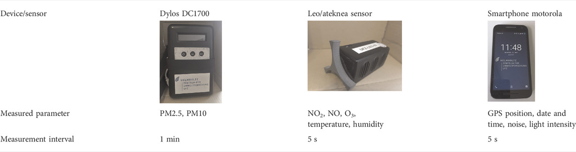
TABLE 1. Sensor set for the measurement campaign 2020.

Particulate matter is measured in different sizes (PM2.5 and PM10). The smaller the particle size, the deeper the particles can get into our respiratory system and can cause adverse health effects. Large particles (PM10) can be deposited in the upper airways and medium-sized particles (PM2.5) can be deposited in the lower airways (Falcon-Rodriguez et al., 2016). Noise was measured in dB(A). In order to make it easier for the participants to classify the values, a scale with comparative examples was made available to them (0–20 dB: quiet room, 20–40 dB: entertainment, 40–60 dB: car, 60–80 dB: main street, 80–100 dB: jackhammer, 100–120 dB: pain threshold). The integrated temperature sensor measured the ambient air temperature on routes. The values depend strongly on the weather conditions and differ within the city and over time. In order to make it easier for the participants to classify the values, a scale with comparative examples was made available to them (10–20°C: no temperature stress, 20–26°C: slight temperature stress, 26–32°C: moderate temperature stress, 32–38°C: severe temperature stress, >38°C: extreme temperature stress).

2.4 Unity game engine

We decided to implement an application based on the Unity game engine which meets all the requirements listed in the introduction. Unity provides a development environment for computer games and other interactive 3D graphic applications. The use of the game engine Unity enables us to combine methods from VA and 3D visualization as well as to implement analysis methods and make them available via GUI. As potential users work with different systems, it was important that Unity supports the development of applications for a variety of platforms, including VR environments.

In general, Unity applications consist of one or more scenes, where 3D representatives (so called GameObjects) are presented. With the help of input devices (keyboard, mouse, VR controller), users can move around in the scene and manipulate it via a GUI, for example changing the appearance of GameObjects, removing or adding them.

2.5 Data and data integration

In order to put the data from the mobile sensors into context and to be able to analyse them, a number of additional data sets are integrated into the application. Table 2 gives an overview of these multifaceted datasets and a brief description.

TABLE 2

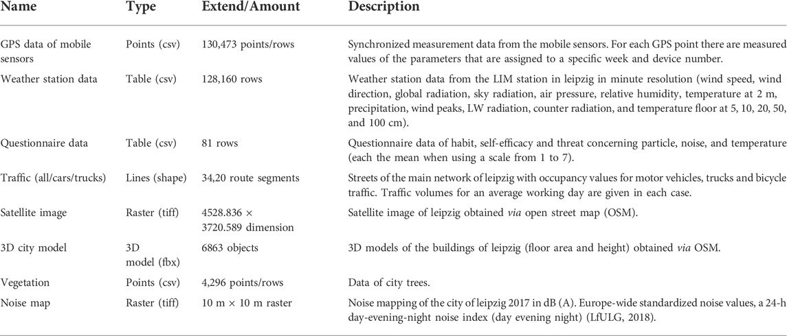
TABLE 2. Integrated data sets.

The data described in the table is read into the Unity application. An interface was implemented for the csv files, through which the measurement data, the vegetation data, the weather data, and the questionnaire data can be read in accordingly and saved as a list of objects of a specific type such as GPS point, tree, weather, and questionnaire data. The other data sets can be read into Unity by default.

The mobile sensor sets (Section 2.3) simultaneously recorded multiple environmental parameters (air temperature, air humidity, particulate matter, ozone, nitrogen oxides, noise, and light). Each measurement refers to a specific time and location registered by the GPS. For this reason, variations in individual measurements may be caused by temporal or spatial changes. For most measurements, it is not possible to decompose the temporal and spatial variations. However, air temperature and humidity clearly follow a diurnal cycle, and this temporal pattern is represented by measurements taken at a fixed station (weather station). Taking advantage of this property, we have removed the daily course from the temperature and humidity measurements, resulting in data ($∆T,∆RH$) that represent only the spatial distribution of temperature and humidity:

$∆T=T_{mobilesensor}-T_{weatherstation}$

$∆RH={RH}_{mobilesensor}-{RH}_{weatherstation}$

The weather station is representative for the urban area and is only influenced by the diurnal cycle (and other variations of the region’s temperature), but not by local building structures. Since the relative humidity is closely related to temperature, we additionally considered the absolute humidity (AH) as a more independent measure of air humidity.

$AH=\frac{RH\bullet \mathrm{6.0328}hPa\bullet e^{\frac{\mathrm{17.1485}\bullet T}{\mathrm{234.69}+T}}}{R\bullet \left(T+\mathrm{273.15}\right)}$

$T$ air temperature in °C$RH$ relative air humidity/100%$R$ gas constant of water (461.52 J/kg/K).

Air pollution and noise data do not follow as clear a diurnal cycle as air temperature, so we did not remove a diurnal course from these measurements. When comparing the measurement data from the campaign with data and maps from other sources, it has to be noted that measurement intervals vary and other methods may have been used for measurement (e.g., number of particles vs. weight of particles in the case of fine dust).

2.6 Data visualization and analysis

We implemented an application that allows to take two perspectives in data analysis: 1) participant and 2) urban area. For the participant analysis, GUI elements were implemented that visualize data at participant level. This includes the questionnaire data on the one hand and personal exposure to various parameters (e.g., temperature) on the other. The exposure is shown for all of a participant’s routes, as well as the minimum, maximum, and average of their total exposure (see Figures 4, 12). For the urban area analysis, all measuring points of the mobile sensors (referred to below as GPS points) are displayed, with either the colour coding, the scaling or both representing the value of the currently selected parameter. By applying analysis methods such as filtering, space time cube, and hot/cold spot calculation, the distribution of stressors within the city can be examined. The methods are described in more detail below.

Users can choose between different perspectives: perspective view, orthographic top view, and orthographic side view. In addition, the individual data layers (each representing a data set, see Section 2.5) can be shown and hidden. The time of the GPS points can be used to display the data in the form of a space time cube. It is possible to use the time of day or the total time since the start of the campaign as the z-value. Due to the shadows cast by the routes, the position of these on the plane can be seen.

In order to be able to display the personal exposure data for each person, it is necessary to assign the individual measuring points to a route, which in turn is assigned to a specific participant (via calendar week and equipment ID). A method has been implemented that allows to connect the individual GPS points according to the routes driven/walked, with the direction indicated by the colour coding (from white to black). All GPS points currently displayed in the scene are included here (hidden, filtered out GPS points are not taken into account). In this context, the application also allows to extract GPS outliers when drawing the routes (also useful for calculating hot/cold spots). Neighbouring GPS points on a route that are at a distance greater than a defined threshold are excluded (see Figure 1).

FIGURE 1

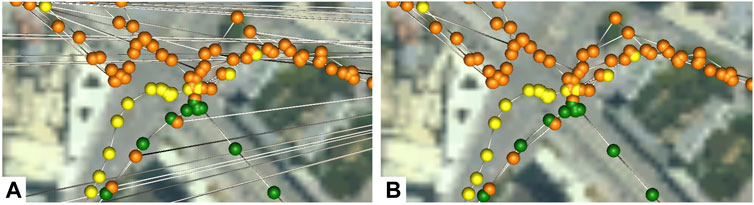
FIGURE 1. GPS points measured with mobile sensors connected according to the driven/walked route (direction from white to black) with GPS outlier (A) and after removing GPS outlier (B).

The absolute values of the measurements from mobile sensors are not calibrated to the same extent as is the case with official measuring stations. That is why we decided to focus on the relative values in our analysis. A method has been implemented that calculates the color-coding of the values according to quantiles of the overall distribution of all values in the data set. For this purpose, a list of all values is created for each parameter during initialization and the quantiles are calculated on this basis and assigned to a colour (see Figure 2).

FIGURE 2

FIGURE 2. Colour coding of measured (top) and calculated (bottom) parameter.

A chained filtering method was implemented for filtering out GPS points of the complete data set by defined value ranges. Several filters can be connected one after the other. Each contains information about the parameter, a minimum, and a maximum value. In addition to filtering by measured values of the GPS points, it is possible to filter by weather parameters (e.g., wind speed).

Time geography was introduced in the seventies and eighties by Hägerstrand (Hägerstrand, 1982) and extended the spatial view of data to include the temporal aspect (Kraak, 2003). Since then, space-time cubes have become a popular method especially for visualising environmental and traffic data (Ahmedi et al., 2022; Yoon and Lee 2021). There is a number of commercial software (e.g., ArcGIS, GeoTime) that supports this method and increased its popularity. For our application we used the approach and implemented a method where the z-axis is used to represent time in 3D space. This means that in addition to the spatial distribution of the measuring points and associated measured values, the temporal aspect can be included in the analysis. Two modes are available for this: on the z-axis 1) the time since the start of the campaign is displayed or 2) the time of day (see Section 3.2 for some examples) in displayed.

In 1992, Getis and Ord developed an algorithm for calculating hot and cold spots of a set of features (in our case points) (Getis and Ord 1992). We implemented a method that calculates Gi* for a selected parameter for all GPS points. For this, the neighbours within a defined radius are calculated for each point (see Figure 3). The z-value for the corresponding GPS point is calculated based on the values of all neighbouring GPS points. In addition, the method can also be applied to a subset (e.g., after filtering) and only takes into account the currently displayed GPS points. In this application, the temporal component is also taken into account when the space-time cube has been applied. In addition to the 2-dimensional spatial neighbourhood, a 3-dimensional one is calculated in which time (on the z-axis) is considered.

$Gi\ast =\frac{{\displaystyle \sum }_{j=\mathrm{1}}^n{w}_{i,j}{x}_j-\overline{X}{\displaystyle \sum }_{j=\mathrm{1}}^n{w}_{i,j}}{S\sqrt{\frac{n{\displaystyle \sum }_{j=\mathrm{1}}^n{w}_{i,j}^{\mathit{2}}-{\left({\displaystyle \sum }_{j=\mathrm{1}}^n{w}_{i,j}\right)}^{\mathrm{2}}}{n-\mathrm{1}}}}\overline{X}=\frac{{\displaystyle \sum }_{j=\mathrm{1}}^n{x}_j}{n}S=\sqrt{\frac{{\displaystyle \sum }_{j=\mathrm{1}}^n{x}_j^{\mathit{2}}}{n}-{\left(\overline{X}\right)}^{\mathit{2}}}$

$x_j$ value for parameter of point j $w_{i,j}$ spatial weight between point i und j.

FIGURE 3

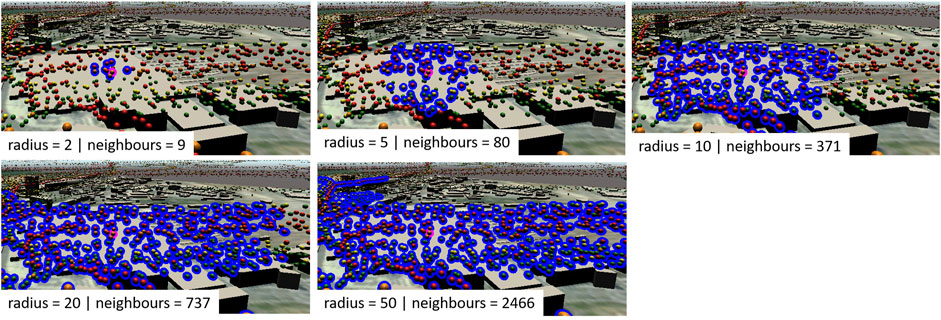
FIGURE 3. Calculated neighbours (blue outline) for an example GPS point (magenta outline) for different radius in space time cube visualization mode.

2.7 Virtual reality environment

The presentation of data in an immersive VR environment increases the perception of domain scientist on the studied scene as well as it enhances the visual understanding of the data analysis process. Therefore, the application was built for and presented in the TESSIN (Terrestrial Environmental System Simulation and Integration Network) VisLab of the UFZ, which is a large-scale interactive multi-audience stereoscopic 3D projection environment that enables users to dive into the data and to explore as well as analyse complex, heterogeneous environmental data (Bilke et al., 2014). The VisLab consists of 13 Digital Light Processing (DLP) projectors and is driven by a multi-GPU (Graphics Processing Unit) visualization server to produce a high-resolution active stereoscopic 3D image on a power wall composed of 4 large-scale projection screens. In addition, a tracking device calculates the relative translation of the viewer against the application origin and adjusts the resulting image position accordingly to immerse the VR perception. A VR controller is used to capture the user input and transmits it to the application for further processing of the intended behaviour.

Unity allows developers to produce a stereoscopic 3D build of their applications. We used the VisLab configuration component of UFZ-Unity-Framework for easy adaptations (Rink et al., 2022a; Rink et al., 2022b). This framework can be used to create Unity scenes by importing heterogeneous environmental data, assign visualization properties to them, and interact with this data by extending the predefined UI components. The UFZ-Unity-Framework includes a VisLab component, which is an extended version of UniCave (Tredinnick et al., 2017). It enables the Unity scenes to be displayed in the VisLab by defining the real-world display configurations. According to the predefined display configurations, it creates virtual cameras to ensure that each projection screen produce the right image seamlessly onto the corresponding screen. Stereoscopic 3D option allows to produce a high resolution active stereoscopic output with doubling the virtual cameras in the scene that are translated by a predefined IPD (inter-pupillary distance) from each other to create two images to be rendered for each eye of the audience. Then, these images alternate in a 120 Hz frequency when they are rendered on the screen with the synchronized shutters of glasses that users wear to obtain the 3D perception. The tracking device captures the location and orientation of the master viewer in the VisLab and broadcast this information over the network, which is received by the server running the Unity application. This process is handled by VRPN which is a device-independent, network-transparent system for accessing virtual reality peripherals from VR applications (Taylor et al., 2001). The location and orientation information is then used by the VisLab component to calculate the relative position and rotation of the master viewer in the Unity scene to align the output image on all output screens. Similarly, the VR controller’s input stream is transmitted to Unity over VRPN and the VisLab component processes the raw input data to locate the pointer and to determine what input signal is received. Then, it triggers the corresponding behaviour.

Our application is configured to run in a single Unity instance to be presented in the main virtual screen (2 of 4 physical screens) in the VisLab which consists of 8 projectors. The GPU driver is employed to create one seamless image of 8 projector outputs. The universal user interface of the application is very complex and therefore not appropriate to use in a VR system. It can be controlled by conventional input devices. On the other hand, navigations in the scene and dataset interactions are handled by the VR controller.

3 Results with discussion

In this chapter we discuss how our approach will help to meet the challenges of data analytics in the future. We present the visualisation and analysis application and address the requirements mentioned in the introduction and how they were met. Afterwards, we give examples to show how the application can be used to test hypotheses and establish new ones.

3.1 Our approach for the future analysis of heterogeneous environmental data

Level of stressors differ very much within a city and we want to investigate the influencing factors. For this purpose, it is necessary to include a large number of additional data (buildings, vegetation, traffic frequency, etc., see Section 2.5). The analysis of this extensive, heterogeneous data is challenging and we follow a combination two approaches: 1) methods of 3D visualisation (using the human ability to grasp visual information very quickly), and 2) statistical methods (aggregation of data to reduce its volume and focus on the essentials). Thereby patterns can be recognised within the city and multiple influencing factors can be identified and quantified. In contrast to conventional approaches (see chapter 1), where island solutions are often used, developed by relatively small development teams, we use an established game engine as the basis for our application. Unity has a large, active community that provides extensive support for development and a large number of free and commercial assets. Thereby it is possible to integrate different data formats with a straightforward development effort and thus enables developers to combine data from different projects generated with different software. In our application, for example, an interface for the integration of csv/txt files was implemented so that these can be accessed directly from the application and no pre-processing by other software is necessary beforehand.

Our approach enables the combination of modern 3D visualisation with various analysis methods. On the one hand, it allows us to provide quicker insight to complex data by showing them in naturally familiar surroundings (e.g., GPS points in 3D model of the city). Thereby people can orientate themselves very quickly, e.g., on the basis of landmarks (e.g., skyscrapers, parks, railway stations). On the other hand, methods for filtering and statistical analysis of the data are provided, which are otherwise only available in software, which in turn provides very limited visualisation methods.

One challenge of visualising heterogeneous, complex environmental data is to facilitate multidisciplinary, collaborative research. By providing methods for presenting the data in a VR environment, we provide an environment that is very well suited for collaborative work. However, it should be noted that navigation in the VR environment is very unfamiliar to many and it requires some training to become more familiar with it and thereby work effectively with it. For example, the devices available for navigation in 3D space (e.g., Flystick) are new to most people, as is the ability to move in three dimensions (as a human being, one usually moves horizontally, vertical movements are only possible with aids). A more natural form of movement would be to walk through the scene as an avatar, but this makes it difficult to get an overall view. Another option is to offer fixed viewpoints that users can access. In our application, three fixed viewpoints have been integrated; besides the bird’s eye view as a good starting point, there is also a direct top view, which provides good orientation, and a side view.

We claim that our approach is suitable for implementing analysis and visualisation tools in future projects, especially collaborative projects and projects with high interdisciplinarity. The trend towards open access and open source of source code in science ensures that developments are made available to each other. In the future, this could lead to some kind of modular system for Unity that can be used as a basis for new projects. Thereby, the development effort can be reduced enormously and multiple use as well as further development of modules can be promoted.

3.2 The application

The application consists of the scene and the GUI elements (requirement a., see Figure 4 for an overview). In the centrally displayed scene, the data is represented by 3D objects (e.g., buildings, vegetation, measuring points). The main menu is located at the top. It can be used to

• select the measurement parameters to be displayed

• change the perspective

• hide and show layers

• switch to the space time cube visualisation mode

• filter the data

• adjust the size of the measurement points

• perform the cold/hot spot calculation (with outlier exclusion, radius definition, and neighbour calculation)

FIGURE 4

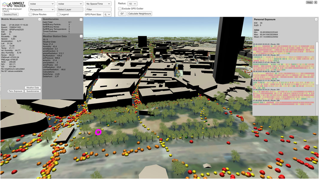
FIGURE 4. Screenshot of the application showing GUI and scene with data (mobile sensing data, buildings, vegetation, and satellite image).

The GUI also displays additional information on the selected measuring point and respectively on the assigned participant:

• Mobile Measurement: parameters measured with the mobile sensors

• Questionnaire data of the participant associated with the measuring point

• Weather Station Data from the Leipzig weather station recorded at the time of the mobile measurement as well as values calculated from both (delta of temperature and humidity)

• Personal exposure of the associated participant to the selected parameter per route with time specification as well as maximum, minimum, and mean value of the total exposure over the complete period.

One requirement was to analyse the data with a smooth performance (requirement b.). However, it should be noted that the frames per second (fps) are lower when all measurement points and additional data sets are displayed. By being able to filter the measurement points directly as well as to easily show and hide additional data sets without extra loading times, methods were provided that allow a temporary and reversible reduction of the data and thus enable a smooth performance. Furthermore, by saving the analysis results (values for cold/hot spot calculations), it is possible to call them up repeatedly without having to spend additional computing time. For example, analyses of different parameters or with different settings can be compared conveniently.

The different data sets are conventionally analysed with different applications and an intersection of the data was thus not possible. The application supports the integration of different data sets (requirement c.) and allows the analysis and the search for causes of patterns that occur, which is shown by the examples given in this chapter. The different representation of the data as 3D objects (requirement d.) ensures that they can be displayed simultaneously without causing occlusion and clutter. A combination of representing the values of one parameter by colour and another by the size of the measurement points (spheres) makes it possible to quickly capture and display relationships between several parameters. The representation of time as a function of altitude makes it possible to compare the values within the campaign time as well as over the course of the day (see examples in Section 3.2).

The use of colour coding according to calculated quantiles for each parameter makes it possible to identify particularly high and low measured values at first glance in relation to the complete measurement campaign. This is especially helpful for viewing the individual load of a participant (see Figures 5, 13). In order to make areas with conspicuous values even more visible, the calculation of cold and hot spots was implemented (requirement e.). Examples in Sections 3.2, 3.3 show application examples of this method.

FIGURE 5

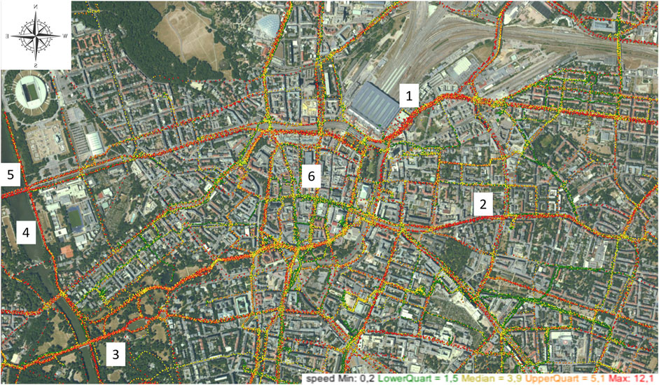
FIGURE 5. Patterns of the speed with which participants moved around the city.

For the visualisation and analysis of the data, the application was exported and run as a Windows program and adapted for VR Lab (requirement f., see Section 3.4). In the following, use cases for the application are described and the results of the analysis are presented and discussed.

3.3 Patterns of the distribution of parameter values in the city

In a first step, the presented application serves to get an overview of the collected mobile data and to analyse its distribution over the city area. Particularly characteristic points in the city are of interest, such as parks, the inner-city ring road, the mostly car-free inner city, in which there is also a ban on cycling during the day. Figure 5 shows the patterns of the speed with which participants moved around the city. A satellite image has been integrated into this display to support orientation and localize green areas and prominent buildings (e.g., main station) easily. Areas or roads with particularly high measured speeds on the routes of the participants can be seen on the main road that runs east past the train station 1), as well as on the parallel main road to the south 2) and to the west in the park 3), as well as along the river 4) and on the main road bridge 5). Lower values can be frequently seen in the inner-city area 6) and on smaller side streets. The measured speed on this overview map is between 0.2 and 12.1 m/s. The analysis of the speed confirms the hypothesis that a higher speed of the participants can be observed in areas with well-developed cycle paths and in parks.

Certain patterns could be recognized in the distribution of nitrogen oxide (NO), which is an indicator for motorized traffic. Figure 6 shows higher values especially around the main station 1) and north-east of it on the main streets 2). Areas of low NO values can be identified mainly in the park 3) and smaller side streets 4). In this representation, the buildings have been integrated to analyse correlations between narrow and wide housing and the distribution of NO. The measured concentration of NO on this overview map is between 0.7 and 676.7 in parts per billion (ppb).

FIGURE 6

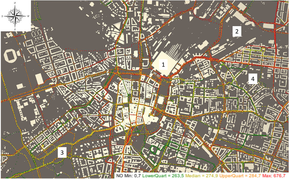
FIGURE 6. Patterns of the NO distribution measured by the mobile sensors.

It could be shown where cyclists are travelling at particularly high speeds. These areas are largely congruent with areas of higher NO pollution. Thus, if cyclists want to drive fast, they have to accept exposure to environmental stressors. The result indicates that promoting cycling infrastructure in side streets (current condition: often no cycle lane, often poor road surface) can have a positive health effect for cyclists. Routes through parks already combine speed and low impact. The use of derelict land (especially along old railway tracks) could be a good addition to create missing “green” connections in the city. This example showed that the application is a very helpful tool for urban planners, as connections can be easily visualised and analysed.

3.4 Impact of time

In order to analyse the extent to which the concentration of environmental stressors depends on the time of day or week in which they were measured, we use the option of displaying time on the z-axis. Figure 7 shows a plot where the campaign time is represented on the z-axis. In the case of routes driven several times, the values can be analysed depending on the calendar week (CW) in which they were travelled. The example shows the absolute measured temperature. It is easy to see which weeks were hotter and which were colder. These observations can then be compared with archive data from the weather stations.

FIGURE 7

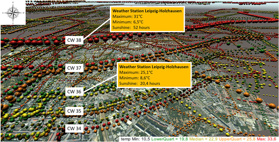
FIGURE 7. Display of the campaign time in the z-axis to identify conspicuous environmental pollution depending on the week they were measured.

Figure 8 shows the calculated cold and hot spots (see Section 2.6) of PM2.5 without (a.) and with representing the time of day in the z-axis (b.). In Figure 8A it can be seen that there are both cold and hot spots in some areas. In order to analyse this more precisely, we use the space-time cube (Figure 8B). Here, an accumulation of cold spots depending on the time of day can be detected. This is particularly visible in the south of the inner city ring road. In the second half of the day, cold spots of particle pollution can be detected. This observation can be made for both PM2.5 and PM10.

FIGURE 8

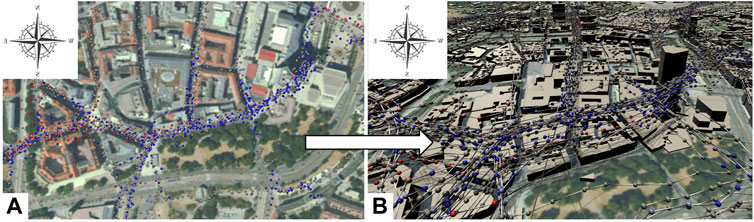
FIGURE 8. Display of the daytime in the z-axis to identify temporal and spatial patterns of environmental pollution (here PM2.5). (A) in 2D and (B) with space time cube visualisation.

In Section 2.5 it is described how the temperature measured by mobile devices is corrected by the temperature measured at the weather station in order to eliminate the natural temperature course of a day. Figure 9 shows the calculated cold and hot spots (see Section 2.6) of ∆T. An accumulation of hotspots depending on the time of day can be seen when applying the space time cube visualisation. This is particularly visible in the area of the inner city ring road, especially in front of the main train station (A) and in the eastern area (B). In the second half of the day, hotspots of ∆T can be detected.

FIGURE 9

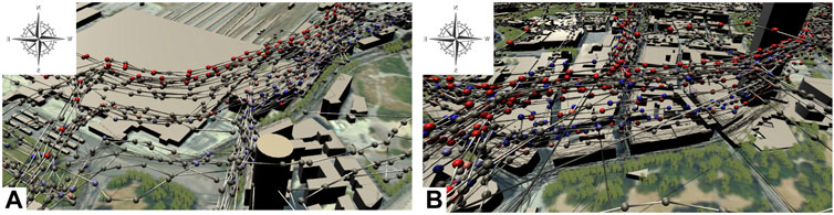
FIGURE 9. Display of the daytime in the z-axis to identify temporal and spatial patterns of urban heat in front of the main train station (A) and in the eastern area (B).

The possibility to display the temperature as a value of the z-axis allows the comparability of different points in time, both when looking at the entire measurement campaign and when analysing the values according to the time of day. It was possible to identify areas with cold spots of PM levels in the second half of the day, which can be explained by an increase in wind at this time of day and thus the transport of PM out of the city. In addition, we identified areas in which heat is particularly stored and whose temperature deviates significantly from that in the surrounding area, especially in the evening and overnight. This shows the potential of the application in the field of urban planning. Areas of the city can be identified where green infrastructure should be created. The effect of this could then again be verified by mobile measurements and integrated into the application for analysis.

When comparing the simulated noise exposure and the measured one by mobile sensors, a high level of correlation could be shown (see Figure 10A), but also differences could be detected, especially in the park. We expected to see noise exposure patterns throughout the day, e.g., higher loads in rush hour times. However, Figure 10B shows that no patterns can be seen in the temporal distribution of the hotspots (z-axis).

FIGURE 10

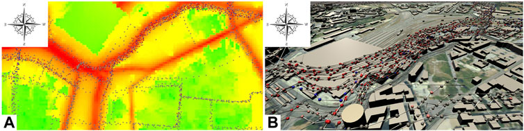
FIGURE 10. Comparison of simulated and measured noise pollution (A) and display of the daytime in the z-axis to identify temporal and spatial patterns of noise (B).

This example shows the current limitations of the application. By implementing additional analysis methods (e.g., statistical methods), these can be eliminated. The fact that no patterns could be detected for the parameter noise related with time of day could be due to the fact that multiple influencing factors play a role here (e.g., speed, wind speed, wind direction in combination with the direction of the road, time of day, road type). Causality algorithms can be implemented to identify these more complex correlations, in the future.

3.5 Outlier analysis

One task that the application aims to process is the analysis of outliers. It should be investigated for which parameters these are present and the reasons for their occurrence should be analysed. Figure 11B. shows the analysis of the hot and cold spots for NO. Here we can get a first impression of where cold and hotspots are located. In order to make the outliers clearly visible, it is required to scale the spheres according to their values. In Figure 11A it can be seen that the cold spot outliers are in three areas. To find the cause of the outlier values, we compared the additional data on these points. For all three areas, the values of specific participants are responsible, which can be clearly identified by the calendar week (CW) and the equipment ID. The equipment ID is different for everyone, which means that an inaccurate calibration of the gas sensor can be ruled out as the cause. We could not find any abnormalities in the other parameters measured. Likewise, when looking at the values of the weather station for these three examples, no abnormalities could be identified. When examining the participants’ personal exposure to NO, it was found that these contained both minimum and maximum values, but that two had a disproportionate accumulation of minimum values (see Figure 12). In addition, the questionnaire data of the respective participants were considered in order to analyse whether a particularly high protective behaviour of the participants was indicated, which could explain the values. This could not be proven. Including measures of perceived threat and coping abilities can contextualize individuals routing choices. Including questionnaire data on participants’ intentions to choose routes with low pollution can also help to analyse whether their intentions align with their actual route choices and the respective pollution levels. Furthermore, the questionnaire included questions on routing habits. These can also help to contextualize people’s route choices. Urban planners can take this information into account when planning bike lanes that are not only low in pollution levels, but also align with user preferences and habits.

FIGURE 11

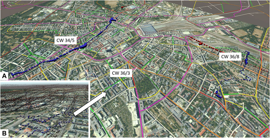
FIGURE 11. Identification of outliers, e.g., cold spots of NO concentration for three participants using representation of value by colour and size (in addition simulated traffic is shown as lines). (A) with size by value and (B) without size by value.

FIGURE 12

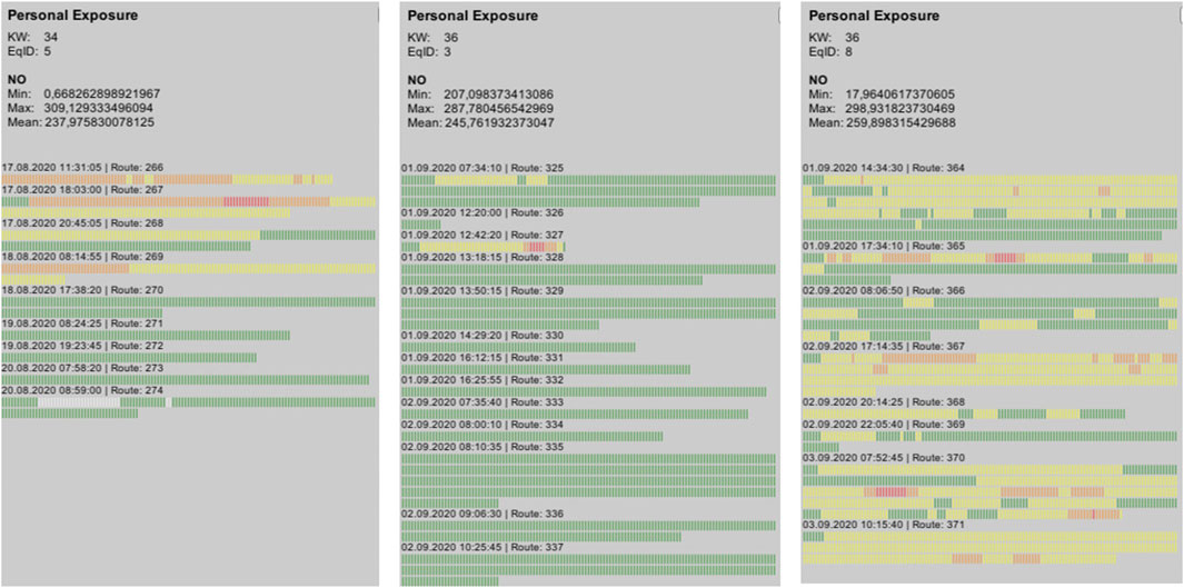
FIGURE 12. Personal exposure in total (top) and per route (below) to NO of participants with outlier values.

This example shows the current limitations of the application, which can be addressed, for example, by integrating additional data (e.g., socio-economic data) and thus identify reasons for the appearance of outliers.

3.6 Presentation in virtual reality lab

The implemented application was adapted for presentation in the VR lab of the UFZ (see Section 2.7) and tested there in several sessions. In addition, an analysis session was held with project members in May 2022 to review the results, where it turned out that the application was a very good way for experts in the domain to examine the data in detail. Especially the representation in the space time cube becomes even more vivid and intuitive in the VR environment, especially paired with the representation of the routes. Furthermore, a workshop with stakeholders from different areas took place focusing on the topic heat stress (Figure 13). The application provided these stakeholders with a quick and comprehensible insight into the project data. Further requirements could also be identified in the discussion, for example, information on specific buildings (schools, hospitals, care facilities) would be helpful, because vulnerable groups of people are exposed to stressors there.

FIGURE 13

FIGURE 13. Presentation of the visualization and analysis application during a workshop with stakeholders in the VR environment TESSIN VisLab (Photos: Özgür Ozan Sen).

This form of presentation is particularly suitable for interdisciplinary research and interdisciplinary discussions in general, and thus functions as a boundary object between the disciplines. It should be noted that an appropriately large time frame should be planned for these sessions in order to allow the participants a certain familiarisation phase with the VR environment.

4 Conclusion and outlook

In this paper we presented a visualisation and analysis application for environmental mobile sensor data in an urban context. The analysis of a measurement campaign was used to show how the application can be used in practice and what added value it brings compared to conventional applications. The application enables merging different data/sources (Urban 3D structure, sensor data, weather data, questionnaire data) and apply spatial analysis algorithm (Getis Ord Gi*) including neighbour calculation in space and time. The analysis of the distribution of the data over the city is possible as well as the analysis of the exposure to environmental stressors of a single individual. The possibility to use the application on a PC as well as in the VR environment makes it versatile (e.g., analysis sessions by experts/non-experts, workshops with stakeholders/citizens). The application has achieved the goal of meeting all requirements. However, it should also be noted that the design and implementation of such a customised tool also implies a certain development effort.

We claim that our approach should be used for implementing analysis and visualisation tools in future projects, because of these aspects:

(1) It has the potential to become a modular system for applications by reusing and further developing methods (utilize open access and open source resources).

(2) It enables the combination of modern 3D visualisation with various analysis methods.

(3) It supports presentation in VR environments and thereby facilitates multidisciplinary, collaborative research in collaborative projects and projects with high interdisciplinarity.

Our work has shown the importance of adequate tools for analysing environmental data. The results showed how areas can be identified where improvements in terms of conditions for cycling and walking are required. In the future, the integration of real time data into the application would be interesting in order to quickly detect changes (e.g., through the creation of green infrastructure in certain areas) and to take short-term measures in acute cases (e.g., severe heatwave). In addition, it should be investigated whether there are patterns in individual exposure in connection with socio-economic data of the individual, or route lengths and city districts. We also want to test other visualisation methods, such as continuous surface to show and compare pollutant levels. The calculation and presentation of uncertainties in the measurements is also a priority for future work.

Another future application for the tool is in psychological studies where test persons could drive routes in the VR environment and the corresponding level of environmental stressors is visualised. Specifically, future studies may investigate if providing information about environmental stressors in VR environments will affect perceptions of personal environmental health risks and—subsequently—influence participants’ mobility behavior intentions (e.g., routing behavior). Intriguingly, applying a VR environment may even offer an opportunity to test participants’ routing behavior choices more directly. For example, future studies may provide participants with information about their personal exposure to environmental stressors on their daily trips. Following this, respondents could be asked to choose between different routes to drive/ride in the VR environment, involving different levels of exposure to environmental stressors and different opportunity costs (e.g., travel time). This could complement or even replace field studies in the future.

Data availability statement

The application presented in this paper can be found at the Data Investigation Portal of the UFZ: https://www.ufz.de/record/dmp/archive/12713/en/. In order to preserve the anonymity of our measurement study participants, information on the measurement week, measurement equipment and measurement time was removed from the data set. This means that some of the functions described in the paper (e.g., space time cube visualisation, show routes) are not available in the provided version.

Ethics statement

The exploratory study was approved by the local ethics committee of the Leipzig University (No. 191/17-ek), and all volunteers signed a written informed consent for us to record sensitive GPS travel data.

Author contributions

CH was the principal author for the text, responsible for editing the whole manuscript together, and responsible for the concept and implementation of the visualisation and analysis application. Other authors contributed to the measurement campaign and data sampling (AB, AM), implementing VR interfaces (OS) and also contributed specific sections of text (all).

Funding

The research was supported by the funding from DGF in VGI Science program (contract number SCHL521/8-1).

Acknowledgments

We acknowledge Dieter Auspurg and Frank Findeisen from the city of Leipzig for providing traffic data, Cyrill Rasch from the city of Leipzig for providing noise map, Heidrun Gebhardt from the city of Leipzig and Sebastian Elze from UFZ for providing vegetation data, Florian Schmidt for the implementation of the smartphone app for the measurement campaign, and Sophie Schmidt from UFZ for help editing the manuscript. We thank the library of the UFZ for financing the publication costs.

Conflict of interest

The authors declare that the research was conducted in the absence of any commercial or financial relationships that could be construed as a potential conflict of interest.

Publisher’s note

All claims expressed in this article are solely those of the authors and do not necessarily represent those of their affiliated organizations, or those of the publisher, the editors and the reviewers. Any product that may be evaluated in this article, or claim that may be made by its manufacturer, is not guaranteed or endorsed by the publisher.

References

Adams, M. D., and Kanaroglou, P. S. (2016). Mapping real-time air pollution health risk for environmental management: Combining mobile and stationary air pollution monitoring with neural network models. J. Environ. Manag. 168, 133–141. doi:10.1016/j.jenvman.2015.12.012

PubMed Abstract | CrossRef Full Text | Google Scholar

Adagha, O., Levy, R. M., Carpendale, S., Gates, C., and Lindquist, M. (2017). Evaluation of a visual analytics decision support tool for wind farm placement planning in Alberta: Findings from a focus group study. Technological Forecasting and Social Change 117, 70–83. doi:10.1016/j.techfore.2017.01.007

CrossRef Full Text | Google Scholar

Ahmadi, H., Argany, M., Ghanbari, A., and Ahmadi, M. (2022). Visualized spatiotemporal data mining in investigation of Urmia Lake drought effects on increasing of PM10 in Tabriz using Space-Time Cube (2004–2019). Sustainable Cities and Society. 76, 103399. doi:10.1016/j.scs.2021.103399

CrossRef Full Text | Google Scholar

Anwar, A., Ayub, M., Khan, N., and Flahault, A. (2019). Nexus between air pollution and neonatal deaths: A case of asian countries. Int. J. Environ. Res. Public Health 17 (21), 4148. doi:10.3390/ijerph16214148

CrossRef Full Text | Google Scholar

Arnstein, S. R. (1969). A ladder of citizen participation. J. Am. Inst. Planners 35 (4), 216–224. doi:10.1080/01944366908977225

CrossRef Full Text | Google Scholar

Avazpour, I., Grundy, J., and Zhu, L. (2019). Engineering complex data integration, harmonization and visualization systems. J. Industrial Information Integration 16, 100103. doi:10.1016/j.jii.2019.08.001

CrossRef Full Text | Google Scholar

Bakolis, I., Hammoud, R., Stewart, R., Beevers, S., Dajnak, D., MacCrimmon, S., et al. (2021). Mental health consequences of urban air pollution: Prospective population-based longitudinal survey. Soc. Psychiatry Psychiatr. Epidemiol. 56 (9), 1587–1599. doi:10.1007/s00127-020-01966-x

PubMed Abstract | CrossRef Full Text | Google Scholar

Becker, A. M., Marquart, H., Masson, T., Helbig, C., and Schlink, U. (2021). Impacts of Personalized Sensor Feedback Regarding Exposure to Environmental Stressors. Curr. Pollution Rep. 7 579–593. doi:10.1007/s40726-021-00209-0

CrossRef Full Text | Google Scholar

Behrens, U., and Hoffmann, K. (2016). Bericht - stadtklimatische Untersuchungen in Leipzig. Ergebnisse statistischer Auswertungen langjähriger Klimareihen sowie temporärer Stations- und Profilmessungen. Potsdam: Deutscher Wetterdienst Potsdam. URL: https://www.dwd.de/DE/klimaumwelt/klimaforschung/klimawirk/stadtpl/stadtklimaprojekte/projekt_leipzig/externe_links/ergebnisse.pdf?__blob=publicationFile&v=2 May Access 18, 2022).

Google Scholar

Berger, M., and Bill, R. (2019). Combining VR visualization and sonification for immersive exploration of urban noise standards. Multimodal Technol. Interact. 3, 34. doi:10.3390/mti3020034

CrossRef Full Text | Google Scholar

Bilke, L., Fischer, T., Helbig, C., Krawczyk, C., Nagel, T., Naumov, D., et al. (2014). TESSIN VISLab—Laboratory for scientific visualization. Environ. Earth Sci. 72 (10), 3881–3899. doi:10.1007/s12665-014-3785-5

CrossRef Full Text | Google Scholar

Boogaard, H., Walker, K., and Cohen, A. J. (2019). Air pollution: The emergence of a major global health risk factor. Int. Health 11 (6), 417–421. doi:10.1093/inthealth/ihz078

PubMed Abstract | CrossRef Full Text | Google Scholar

Bonney, R., Phillips, T. B., Ballard, H. L., and Enck, J. W. (2016). Can citizen science enhance public understanding of science?. Public Underst. Sci. 25(1), 2–16. doi:10.1177/0963662515607406

PubMed Abstract | CrossRef Full Text | Google Scholar

Brooks, F. P. (1999). What's real about virtual reality?. IEEE Computer Graphics and Applications 19(6), 16–27. doi:10.1109/38.799723

CrossRef Full Text | Google Scholar

M. Budde, T. Riedel, M. Beigl, K. Schäfer, S. Emeis, J. Cyryset al. (Editors) (2017). SmartAQnet: remote and in-situ sensing of urban air quality. SPIE Remote Sensing. Washington, DC: SPIE.

Google Scholar

Bundesamt für Justiz (2022). Gesetz zum Schutz vor schädlichen Umwelteinwirkungen durch Luftverunreinigungen, Geräusche, Erschütterungen und ähnliche Vorgänge. Bonn: Bundesministerium für Justiz. URL: https://www.gesetze-im-internet.de/bimschg/ May Access 18, 2022).

Google Scholar

Burdea, G. C., and Coiffet, P. (2003). Virtual Reality Technology. New Jersey: Wiley.

Google Scholar

Cai, Y. T., Ramakrishnan, R., and Rahimi, K. (2021). Long-term exposure to traffic noise and mortality: A systematic review and meta-analysis of epidemiological evidence between 2000 and 2020. Environ. Pollut. 269, 116222. doi:10.1016/j.envpol.2020.116222

PubMed Abstract | CrossRef Full Text | Google Scholar

Cao, T., and Thompson, J. E. (1905). Personal monitoring of ozone exposure: A fully portable device for under $150 USD cost. Sens. Actuators B. Chem. 224 936–943. doi:10.1016/j.snb.2015.10.090

CrossRef Full Text | Google Scholar

Chatzidiakou, L., Krause, A., Popoola, O. A. M., Di Antonio, A., Kellaway, M., Han, Y., et al. (2019). Characterising low-cost sensors in highly portable platforms to quantify personal exposure in diverse environments. Atmos. Meas. Tech. 12, 4643–4657. doi:10.5194/amt-12-4643-2019

PubMed Abstract | CrossRef Full Text | Google Scholar

Chizhova, M., Popovas, D., Gorkovchuk, D., Gorkovchuk, J., Hess, M., and Luhmann, T. (2020). Virtual terrestrial laser scanner simulator for digitalisation of teaching environment: Concept and first results. Int. Arch. Photogramm. Remote Sens. Spat. Inf. Sci. XLIII-B5-2020, 91–97. doi:10.5194/isprs-archives-XLIII-B5-2020-91-2020

CrossRef Full Text | Google Scholar

Cui, Z., Henrickson, K., Biancardo, S. A., Pu, Z., and Wang, Y. (2020). Establishing multisource data-integration framework for transportation data analytics. J. Transport. Enng., Part A: Syst. 146, 04020024. doi:10.1061/JTEPBS.0000331

CrossRef Full Text | Google Scholar

De Troeyer, K., Bauwelinck, M., Aerts, R., Profer, D., Berckmans, J., Delcloo, A., et al. (2020). Heat related mortality in the two largest Belgian urban areas: A time series analysis. Environ. Res. 188, 109848. doi:10.1016/j.envres.2020.109848

PubMed Abstract | CrossRef Full Text | Google Scholar

EUR-Lex (2008). Directive 2008/50/EC of the European Parliament and of the Council of 21 May 2008 on ambient air quality and cleaner air for Europe. Official J. L152 51, 169–212.

Google Scholar

Eitzel, M. V., Cappadonna, J. L., Santos-Lang, C., Duerr, R. E., Virapongse, A., West, S. E., et al. (2017). Citizen science terminology matters: Exploring key terms. Citizen Science: Theory and Practice 2 (1), 1. doi:10.5334/cstp.96

CrossRef Full Text | Google Scholar

Falcon-Rodriguez, C. I., De Vizcaya-Ruiz, A., Rosas-Pérez, I. A., Osornio-Vargas, Á. R., and Segura-Medina, P. (2017). Inhalation of concentrated PM2.5 from Mexico City acts as an adjuvant in a guinea pig model of allergic asthma. Environ. Pollut. 228, 474–483. doi:10.1016/j.envpol.2017.05.050

PubMed Abstract | CrossRef Full Text | Google Scholar

Friedhoff, R., and Kiely, T. (1990). The eye of the Beholder. Computer Graphics World 13 (8), 46–56.

Google Scholar

Fusco, G., and Aversano, L. (2020). An approach for semantic integration of heterogeneous data sources. PeerJ Comput. Sci. 6 (2). doi:10.7717/peerj-cs.254

CrossRef Full Text | Google Scholar

Gaskins, A. J., and Hart, J. E. (2019). The use of personal and indoor air pollution monitors in reproductive epidemiology studies. Paediatr. Perinat. Epidemiol. doi:10.1111/ppe.12599

CrossRef Full Text | Google Scholar

Getis, A., and Ord, J. K. (1992). The analysis of spatial association by use of distance statistics. Geogr. Anal. 24, 189–206. doi:10.1111/j.1538-4632.1992.tb00261.x

CrossRef Full Text | Google Scholar

Gershon, N., and Eick, S. (1995). Foreword. In: Proc. IEEE symp. Information Visualization (InfoVis 95) (IEEE CS Press) vii–viii.

Google Scholar

Guillaume, G., Aumond, P., Chobeau, P., and Can, A. (2019). Statistical study of the relationships between mobile and fixed stations measurements in urban environment. Build. Environ. 149, 404–414. doi:10.1016/j.buildenv.2018.12.014

CrossRef Full Text | Google Scholar

Haddad, N., Andrianou, X. D., and Makris, K. C. (2019). A scoping review on the characteristics of human exposome studies. Curr. Pollut. Rep. 5 (3), 378–393. doi:10.1007/s40726-019-00130-7

CrossRef Full Text | Google Scholar

Hägerstrand, T. (1982). Diorama, Path AND Project. Tijdschr. Econ. Soc. Geogr. 73, 323–339. doi:10.1111/j.1467-9663.1982.tb01647.x

CrossRef Full Text | Google Scholar

Haklay, M. (2013). “Citizen science and volunteered geographic information: Overview and typology of participation,” in Crowdsourcing geographic knowledge. Editors D. Sui, S. Elwood, and M. Goodchild (Dordrecht: Springer). doi:10.1007/978-94-007-4587-2_7

CrossRef Full Text | Google Scholar

Haklay, M. (2018). “Participatory citizen science,” in Citizen science: Innovation in open science, society and policy (London: UCL Press), 52–62.

CrossRef Full Text | Google Scholar

Hauser, H., and Kehrer, J. (2013). Visualization and visual analysis of multifaceted scientific data: A survey. IEEE Trans. Vis. Comput. Graph. 19 (3), 495–513. doi:10.1109/TVCG.2012.110

PubMed Abstract | CrossRef Full Text | Google Scholar

Helbig, C., Bilke, L., Bauer, H. S., Böttinger, M., and Kolditz, O. (2015). Meva - an interactive visualization application for validation of multifaceted meteorological data with multiple 3D devices. PLoS ONE 10 (4), e0123811. doi:10.1371/journal.pone.0123811

PubMed Abstract | CrossRef Full Text | Google Scholar

Helbig, C., Dransch, D., Böttinger, M., Devey, C., Haas, A., Hlawitschka, M., et al. (2017). Challenges and strategies for the visual exploration of complex environmental data. Int. J. Digital Earth 10 (10), 1070–1076. doi:10.1080/17538947.2017.1327618

CrossRef Full Text | Google Scholar

Helbig, C., Ueberham, M., Becker, A. M., Marquart, H., and Schlink, U. (2021). “Wearable Sensors for Human Environmental Exposure in Urban Settings,” in Current Pollution Reports. doi:10.1007/s40726-021-00186-4

CrossRef Full Text | Google Scholar

Hruby, F. (2019). The sound of being there: Audiovisual cartography with immersive virtual environments. Kn. J. Cartogr. Geogr. Inf. 69, 19–28. doi:10.1007/s42489-019-00003-5

CrossRef Full Text | Google Scholar

Irwin, A. (1995). Citizen Science: A Study of People, Expertise, and Sustainable Development. New York: Routledge.

Google Scholar

Kraak, M.-J. (2003). Geovisualization illustrated. ISPRS J. Photogramm. Remote Sens. 57 (5–6), 390–399. doi:10.1016/S0924-2716(02)00167-3

CrossRef Full Text | Google Scholar

Keil, J., Edler, D., Schmitt, T., and Dickmann, F. (2021). Creating immersive virtual environments based on open geospatial data and game engines. Kn. J. Cartogr. Geogr. Inf. 71, 53–65. doi:10.1007/s42489-020-00069-6

CrossRef Full Text | Google Scholar

Kumar, P., Druckman, A., Gallagher, J., Gatersleben, B., Allison, S., Eisenman, T. S., et al. (2019). The nexus between air pollution, green infrastructure and human health. Environ. Int. 133 (A), 105181. doi:10.1016/j.envint.2019.105181

PubMed Abstract | CrossRef Full Text | Google Scholar

Laksono, D., and Aditya, T. (2019). Utilizing A game engine for interactive 3D topographic data visualization. ISPRS Int. J. Geoinf. 8 (3), 361. doi:10.3390/ijgi8080361

CrossRef Full Text | Google Scholar

Landesamt für Umwelt, Landwirtschaft und Geologie (2018). Hinweise für die Strategische Lärmkartierung - hilfestellung zur Interpretation der Ergebnisse der Lärmkartierung im Internet-Kartendienst des LfULG’. Dresden: Freistaat Sachsen. URL: http://www.umwelt.sachsen.de/umwelt/download/laerm_licht_mobilfunk/Merkblatt_Interpretation_Laermkarten.pdf May Access 18, 2022).

Google Scholar

Leipziger Institut für Meteorologie (2022). ’Aktuelle Zeitreihen (Minutenmittel der letzten 48h)’. Leipzig: Leipziger Institut für Meteorologie - LIM. URL: https://wetterdaten.meteo.uni-leipzig.de/ May Access 18, 2022).

Google Scholar

Lu, X., Tomkins, A., Hehl-Lange, S., and Lange, E. (2021). Finding the difference: Measuring spatial perception of planning phases of high-rise urban developments in Virtual Reality. Computers, Environment and Urban Systems 90, 101685. doi:10.1016/j.compenvurbsys.2021.101685

CrossRef Full Text | Google Scholar

Luigi, M., Massimiliano, M., Aniello, P., Gennaro, R., and Virgina, P. R. (2015). On the validity of immersive Virtual Reality as tool for multisensory evaluation of Urban Spaces. Energy Procedia 78, 471–476. doi:10.1016/j.egypro.2015.11.703

CrossRef Full Text | Google Scholar

McCormick, B. H., DeFanti, T. A., and Brown, M. D. (1991). Visualization in scientific computing. Computer Graphics 21 (6). doi:10.1016/S0065-2458(08)60168-0

CrossRef Full Text | Google Scholar

Mitsakou, C., Dimitroulopoulou, S., Heaviside, C., Katsouyanni, K., Samoli, E., Rodopoulou, S., et al. (2019). Environmental public health risks in European metropolitan areas within the EURO-HEALTHY project. Sci. Total Environ. 658, 1630–1639. doi:10.1016/j.scitotenv.2018.12.130

PubMed Abstract | CrossRef Full Text | Google Scholar

Mokas, I., Lizin, S., Brijs, T., Witters, N., and Malina, R. (2021). Can immersive virtual reality increase respondents’ certainty in discrete choice experiments? A comparison with traditional presentation formats. Journal of Environmental Economics and Management 109, 102509. doi:10.1016/j.jeem.2021.102509

CrossRef Full Text | Google Scholar

Mueller, N., Rojas-Rueda, D., Khreis, H., Cirach, M., Andres, D., Ballester, J., et al. (2020). Changing the urban design of cities for health: The superblock model. Environ. Int. 134, 105132. doi:10.1016/j.envint.2019.105132

PubMed Abstract | CrossRef Full Text | Google Scholar

Munzel, T., Steven, S., Frenis, K., Lelieveld, J., Hahad, O., and Daiber, A. (2020). Environmental factors such as noise and air pollution and vascular disease. Antioxid. Redox Signal. 33 (9), 581–601. doi:10.1089/ars.2020.8090

PubMed Abstract | CrossRef Full Text | Google Scholar

Nadrian, H., Mahmoodi, H., Taghdisi, M. H., Aghemiri, M., Babazadeh, T., Ansari, B., et al. (2020). Public health impacts of urban traffic jam in sanandaj, Iran: A case study with mixed-method design. J. Transp. Health 19, 100923. doi:10.1016/j.jth.2020.100923

CrossRef Full Text | Google Scholar

Nazemi, M., van Eggermond, M. A. B., Erath, A., Schaffner, D., Joos, M., and Axhausen, K. W. (2021). Studying bicyclists perceived level of safety using a bicycle simulator combined with immersive virtual reality. Accident Analysis & Prevention 151, 105943. doi:10.1016/j.aap.2020.105943

CrossRef Full Text | Google Scholar

Nieuwenhuijsen, M. J. (2021). Green infrastructure and health. Annu. Rev. Public Health 42, 317–328. doi:10.1146/annurev-publhealth-090419-102511

PubMed Abstract | CrossRef Full Text | Google Scholar

Nieuwenhuijsen, M., and Khreis, H. (2018). “Urban and transport planning, environment and health,” in Integrating human health into urban and transport planning, 3–16. doi:10.1007/978-3-319-74983-9_1

CrossRef Full Text | Google Scholar

Oresic, M., McGlinchey, A., Wheelock, C. E., and Hyotylainen, T. (2020). Metabolic signatures of the exposome-quantifying the impact of exposure to environmental chemicals on human health. Metabolites 10 (11), 454. doi:10.3390/metabo10110454

CrossRef Full Text | Google Scholar

Oxford English dictionary (2020). https://www.oed.com/view/Entry/33513?redirectedFrom=citizen+science (Accessed March 19, 2020)

Pei, L. (2021). Green urban garden landscape design and user experience based on virtual reality technology and embedded network. Environmental Technology & Innovation 24, 101738. doi:10.1016/j.eti.2021.101738

CrossRef Full Text | Google Scholar

Rafiee, A., Van der Male, P., Dias, E., and Scholten, H. (2017). Developing a wind turbine planning platform: Integration of “sound propagation model–GIS-game engine” triplet. Environ. Model. Softw. 95, 326–343. ISSN 1364-8152. doi:10.1016/j.envsoft.2017.06.019

CrossRef Full Text | Google Scholar

Regueiro, M. A., Viqueira, J. R. R., Taboada, J. A., and Cotos, J. M. (2015). Virtual integration of sensor observation data. Comput. & Geosci. 81, 12–19. doi:10.1016/j.cageo.2015.04.006

CrossRef Full Text | Google Scholar

Rink, K., Şen, Ö. O., Hannemann, M., Ködel, U., Nixdorf, E., Weber, U., et al. (2022a). An environmental exploration system for visual scenario analysis of regional hydro-meteorological systems. Comput. Graph. 103, 192–200. doi:10.1016/j.cag.2022.02.009

CrossRef Full Text | Google Scholar

Rink, K., Şen, Ö. O., Schwanebeck, M., Hartmann, T., Gasanzade, F., Nordbeck, J., et al. (2022b). An environmental information system for the exploration of energy systems. Geotherm. Energy 10 (1), 4–16. doi:10.1186/s40517-022-00215-5

CrossRef Full Text | Google Scholar

Schmohl, S., Tutzauer, P., and Haala, N. (2020). Stuttgart city walk: A case study on visualizing textured dsm meshes for the general public using virtual reality. PFG 88, 147–154. doi:10.1007/s41064-020-00106-z

CrossRef Full Text | Google Scholar

Schuster, C., Honold, J., Lauf, S., and Lakes, T. (2017). Urban heat stress: Novel survey suggests health and fitness as future avenue for research and adaptation strategies. Environ. Res. Lett. 12 (4), 044021. doi:10.1088/1748-9326/aa5f35

CrossRef Full Text | Google Scholar

Sinha, P., Coville, R. C., Hirabayashi, S., Lim, B., Endreny, T. A., and Nowak, D. J. (2021). Modeling lives saved from extreme heat by urban tree cover? Ecol. Model. 449, 109553. doi:10.1016/j.ecolmodel.2021.109553

CrossRef Full Text | Google Scholar

Simpson, R., LaViola, J., Laidlaw, D., Forsberg, A., and van Dam, A. (2000). Immersive VR for scientific visualization: a progress report. IEEE Computer Graphics and Applications 20 (6), 26–52. doi:10.1109/38.888006

CrossRef Full Text | Google Scholar

Stadt Leipzig (2018). ‘Luftreinhalteplan für die Stadt Leipzig - fortschreibung 2018’. Leipzig: Stadt Leipzig. URL: https://www.luft.sachsen.de/download/luft/LRP_Leipzig-2018_Fassung_14-5-2019.pdf May Access 18, 2022).

Google Scholar

Stadt Leipzig (2022a). Ergebnisse der Online-Befragung während des Lärmforums 2011. Leipzig: Stadt Leipzig. URL: https://static.leipzig.de/fileadmin/mediendatenbank/leipzig-de/Stadt/02.3_Dez3_Umwelt_Ordnung_Sport/36_Amt_fuer_Umweltschutz/Luft_und_Laerm/Laermschutz/Laermaktionsplan/laermforum2011_umfrage_ergebnisse.pdf May 18, 2022).Access

Google Scholar

Stadt Leipzig (2022b). Feinstaub - infos und aktuelle Werte in Leipzig. Leipzig: Stadt Leipzig. URL: https://www.leipzig.de/umwelt-und-verkehr/luft-und-laerm/luftreinhaltung/luftschadstoffe-und-grenzwerte/feinstaub May Access 18, 2022).

Google Scholar

Stadt Leipzig (2022c). Lärmkartierung und Berechnungsvorschriften. Leipzig: Stadt Leipzig. URL: https://www.leipzig.de/umwelt-und-verkehr/luft-und-laerm/laermschutz/laermkartierung-und-berechnungsvorschriften#c30111 May Access 18, 2022).

Google Scholar

Strasser, B. J., Baudry, J., Mahr, D., Sanchez, G., and Tancoigne, E. (2019). Citizen science’? Rethinking science and public participation. Sci. Technol. Stud. 32 (2), 52–76. doi:10.23987/sts.60425

CrossRef Full Text | Google Scholar

Taylor, R. M., Hudson, T. C., Seeger, A., Weber, H., Juliano, J., and Helser, A. T. (2001). “Vrpn: A device-independent, network-transparent VR peripheral system,” in Proceedings of the ACM symposium on Virtual reality software and technology, 55–61.

Google Scholar

Tian, C., and Li, G. (2019). A framework for the data integration of earthquake events. IEEE Access 7, 172628–172637. doi:10.1109/ACCESS.2019.2957024

CrossRef Full Text | Google Scholar

Tredinnick, R., Boettcher, B., Smith, S., Solovy, S., and Ponto, K. (2017). “Uni-CAVE: A Unity3D plugin for non-head mounted VR display systems,” in Proceeding of the 2017 IEEE Virtual Reality (VR), Los Angeles, CA, USA, March 2017 (IEEE), 393–394.

CrossRef Full Text | Google Scholar

Trumble, B. C., and Finch, C. E. (2019). The exposome in human evolution: From dust to diesel. Q. Rev. Biol. 94 (4), 333–394. doi:10.1086/706768

PubMed Abstract | CrossRef Full Text | Google Scholar

Tu, D. Q., Kayes, A. S. M., Rahayu, W., and Nguyen, K. (2020). IoT streaming data integration from multiple sources. Computing 102, 2299–2329. doi:10.1007/s00607-020-00830-9

CrossRef Full Text | Google Scholar

Ueberham, M., Schlink, U., Dijst, M., and Weiland, S. (2019). Cyclists’ multiple environmental urban exposures - comparing subjective and objective measurements. Sustainability 11 (5), 1412. doi:10.3390/SU11051412

CrossRef Full Text | Google Scholar

Ueberham, M., and Schlink, U. (2018). Wearable sensors for multifactorial personal exposure measurements – a ranking study. Environ. Int. 121 (1), 130–138. doi:10.1016/j.envint.2018.08.057

PubMed Abstract | CrossRef Full Text | Google Scholar

van Dam, A., Laidlaw, D. H., and Simpson, R. M. (2002). Experiments in immersive virtual reality for scientic visualization. Computers & Graphics 26 (4), 535–555. doi:10.1016/S0097-8493(02)00113-9

CrossRef Full Text | Google Scholar

VGI Science (2022). Environmental volunteered geographic information for personal exposure awareness and healthy mobility behaviour (ExpoAware). URL: https://www.vgiscience.org/projects/expoaware.html August Access 17, 2022).

Google Scholar

Weißmann, M., Edler, D., and Rienow, A. (2022). Potentials of low-budget microdrones: Processing 3D point clouds and images for representing post-industrial landmarks in immersive virtual environments. Front. Robot. AI 9, 886240. doi:10.3389/frobt.2022.886240

PubMed Abstract | CrossRef Full Text | Google Scholar

Yang, L., Zhang, F., Kwan, M.-P., Wang, K., Zuo, Z., Xia, S., et al. (2020). Space-time demand cube for spatial-temporal coverage optimization model of shared bicycle system: A study using big bike GPS data. J. Transp. Geogr. 88, 102861. ISSN 0966-6923. doi:10.1016/j.jtrangeo.2020.102861

CrossRef Full Text | Google Scholar

Yeom, K. (2021). Development of urban air monitoring with high spatial resolution using mobile vehicle sensors. Environ Monit Assess 193, 375. doi:10.1007/s10661-021-09139-2

PubMed Abstract | CrossRef Full Text | Google Scholar

Yoon, J., and Lee, S. (2021). Spatio-temporal patterns in pedestrian crashes and their determining factors: Application of a space-time cube analysis model. Accid. Anal. Prev. 161, 106291. doi:10.1016/j.aap.2021.106291

PubMed Abstract | CrossRef Full Text | Google Scholar

Zeng, W., Fu, C.-W., Müller Arisona, S., Schubiger, S., Burkhard, R., and Ma, K.-L. (2017). A visual analytics design for studying rhythm patterns from human daily movement data. Visual Informatics 1 (2), 81–91. doi:10.1016/j.visinf.2017.07.001

CrossRef Full Text | Google Scholar

Zhang, R.-X., and Zhang, L.-M. (2021). Panoramic visual perception and identification of architectural cityscape elements in a virtual-reality environment. Future Generation Computer Systems 118, 107–117. doi:10.1016/j.future.2020.12.022

CrossRef Full Text | Google Scholar