The traceability of sudden water pollution in river canals based on the pollutant diffusion quantification formula

1 Introduction

Sudden water pollution has a sudden, accidental, more serious impact on its environment, so the first task of emergency disposal of sudden water pollution time is to determine the location of the source of pollution and the intensity of the first time after the incident (Sheng., 2012; Zhang et al., 2010). Sudden water pollution mostly enters the river and canal as a point source and migrates and transforms with the diffusion of the river. The study of the diffusion pattern of pollutants after entering the river canal, and relying on the detection value of pollutant concentration to deduce the location, time, and amount of pollutants put in reverse, is the key to solving the traceability of sudden water pollution (Cheng et al., 2011).

Sudden water pollution traceability is to understand the diffusion process of pollutants after entering a water body. At present, research on sudden water pollution traceability at home and abroad is still in the exploration and development stage (Zhu., 2014), and many scholars have made numerous research results in the identification of pollutant source item information. However, a complete system of sudden water pollution traceability issues has not yet been developed (Charles et al., 2000; Gorelick et al., 2000). There are currently three types of methods for pollutant traceability, the first of which is the use of optimization algorithms to optimally solve for pollutant sources, the second is the use of probabilistic statistical methods, and the third is the method of coupled probability density analysis (Charles et al., 2000). Among the optimization algorithms used, Jha and Datta (2012) used an adaptive simulated annealing algorithm to study the traceability of groundwater pollution, Yuan et al. (2017) studied two-dimensional river water quality parameters using a simplex-particle swarm optimization algorithm, and Xin et al. (2014) used a combination of genetic algorithm and mathematical model for single-point source and multi-point source multivariate problems. Han et al. (2020) proposed a method that couples the dispersion equation of groundwater pollutants with a genetic algorithm (GA) for identifying groundwater pollution sources. Lei et al. (2022) established a new model combining the radial configuration in time (RBCN) method coupled with the differential evolutionary algorithm (DE) for the solution of pollutant source terms and achieved a better solution accuracy. The use of optimization algorithm to solve the pollutant source term can minimize the error of the model simulation and provide a reliable reference for pollution control and treatment of water bodies. Mou et al. (2011) used a differential evolutionary algorithm to study the problem of single and multipoint fixed pollution source term identification. For the second type of method, Yan et al. (2019) proposed an innovative framework based on the Bayesian theory and groundwater pollution source identification, coupling overall linear programming as well as the Markov chain, with better accuracy for the inverse of pollutant source terms. Ghane et al. (2016) solved the pollutant source identification problem in river networks based on the inverse probability density. Yang et al. (2014) transformed the traceability problem into a Bayesian estimation problem to achieve efficient traceability of pollutants. Cao et al. (2010) used Bayesian-Monte Carlo methods to solve the identification problem of the pollution source for the convection-diffusion equation, Chen et al. (2012)used Bayesian-Monte Carlo methods to study the source identification problem of water pollution, and Cheng and Jia (2010) conducted a traceability study of river pollution based on the inverse probability method. Among the coupled probability density optimization methods, Neupauer et al. (2001) used the location and time of the source term of the inverse probability density function sphere; Wang et al. (2015) used probability density analysis coupled with the differential evolution method to conduct a traceability study of sudden water pollution. Kanao and Sato (2022) proposed an edge-sensitivity approach, a time-inverse probabilistic method to estimate the location of pollutant emissions and the time and total amount of pollution from observations of finite elements.

The development of traceability technology can simultaneously quantitatively assess the severity of sudden water pollution events, quickly activate the emergency treatment mechanism for pollution, and efficiently safeguard water resources by quickly capturing the location, time, and discharge quality of such events. Through the use of an assessment index system, numerous academics have recently assessed the state of water resources. To qualitatively evaluate the severity of the lack of water resources, several researchers (Sullivan et al., 2003) developed the hydrological water pressure index and the social water scarcity index. Sun et al. (2020) used the WPI index to assess the level of water poverty in several Chinese provinces; By creating a balance sheet and the multidimensional water poverty (MWP) evaluation system, Yuan et al. (2023) assessed the current state of water resources in Hubei Province and the Yangtze River Economic Belt and examined the issue of a shortage of water resources in Hubei Province and the Yangtze River Economic Belt. The grey water footprint (GWF) and grey water footprint intensity (GWFI) were examined by Kong et al. (2023) to evaluate and analyze the water pollution issue in Jiangsu Province. As can be seen, China continues to face significant problems with its water resources. Traceability technology can offer technological assistance for the preservation of water resources. The essence of the method mentioned in this paper is an improvement in the first type of traceability method mentioned above, and the main objective is to achieve a rapid response to sudden water pollution and to obtain accurate information about the source items of pollutants including the quality, location and time of pollutant discharge. Compared with previous tracking and tracing studies, the proposed tracking and tracing model based on quantitative formulation of diffusion law of pollutants coupled with the improved BAS algorithm is easy to understand and implement. A classic environmental hydraulics inverse problem is the estimation of the traceability of abrupt water contamination (Dooge et al., 2005). A coupled hydrodynamic-water quality model is typically used to simulate the forward calculation of water pollution dispersion. To discretize the collection of St. Venant equations for the hydrodynamic computation, a four-point implicit difference format is used. A one-dimensional convective diffusion equation is derived from water quality calculations based on the conservation of matter principle using the same implicit differential format as the set of equations for discrete computations.

This method in the forward calculation process will exist due to the issue of differential format in the oscillation and non-convergence of the calculation results; to address this issue, the introduction of the pollutant diffusion quantification method on the conventional hydrodynamic-water quality coupled model to simplify the calculation through the physical model to test the quantification method’s reliability to a certain extent. Due to the linked hydrodynamic-water quality model in the reverse calculation of water quality along the propagation of the existence of growing deformation features, the calculation is prone to unstable outcomes throughout the retrospective calculation process. In order to accomplish this, a modified Beetle Antennae Search algorithm based on coupled pollutant diffusion quantification method is suggested. This algorithm converts the conventional differential calculation into the calculation of the system of equations’ optimal solution and significantly speeds up the solution. In the meantime, the traditional BAS algorithm with fixed calculation steps was replaced with the BAS algorithm with variable calculation steps to guarantee the accuracy of the calculation results and to realize the effective and precise traceability of pollutant source parameters.

2 Research methods

2.1 Quantitative methods for pollutant diffusion

After pollutants enter the water, they generally go through three stages: the core zone of the jet, the diffusion zone, and the dispersion zone (Zhang et al., 2005). In this paper, the longitudinal length of the pollutant, the peak transport distance, and the peak concentration of the pollutant are selected as the characteristic parameters of sudden water pollution, and the longitudinal length of the pollutant and the peak transport distance of the pollutant are calculated to determine the extent of pollutant dispersion.

The pollutant concentration can be expressed by the following equation (Long et al., 2016),

$C\left(x,t\right)=C_0\frac{v}{\sqrt{4\pi D_{L}t}}\exp \left(\frac{{\left(x-vt\right)}^2}{4D_{L}t}\right),(1)$

where C (x,t) is the concentration of pollutants at the moment along the x line t, mg/L; C₀ is the concentration of pollution source, mg/L; C₀ = M/Q; M is the total amount of pollutants released instantaneously, g; v is the average flow velocity of the river cross section, m/s, v = Q/A; Q is the river flow, m³/s; A is the cross-sectional area of the river, m²; D_L is the dispersion coefficient, m²/s; x is the distance from the drop point, m.

From Eq. 1, it can be seen that the pollutant concentration is normally distributed according to the normal distribution characteristics, when the pollutant concentration $x=vt$ takes the maximum value, for the channel with low flow rate, the pollutant concentration transfer distance is:

$D=60vT,(2)$

where D is the distance transferred for the pollutant concentration, m; v is the average flow rate of the section, m/s; and T is the propagation time, s.

According to the characteristics of the normal distribution, the dispersion width is defined as $m\sigma$ (m is a constant, $\sigma$ is the standard deviation). The basic idea of determining the dispersion coefficient according to the known tracer method measures the dispersion coefficient in terms of the rate of change of the water mass of the tracer (Najafzadeh et al., 2021).

$D_L=\frac{1}{2}\frac{\partial {\sigma }^2}{\partial t},(3)$

Eq. 3 should be integrated to obtain the longitudinal tensile speed of pollutants,

$v=\frac{m\sigma }{t}=a\sqrt{2}{D_L}^{0.5}{t}^{-0.5},(4)$

where a = m/2.

Integrate Eq. 4 to obtain the longitudinal distance of the pollutant dispersion,

$W={\int }_o^{T}vdt=2a\sqrt{2}{D_L}^{0.5}{T}^{0.5},(5)$

Long (2017) used experimental data obtained from a physical model to fit the longitudinal distance of pollutant dispersion to obtain the empirical equation:

$W=\left[12+\ln \left(\frac{M}{10}\right)\right]\sqrt{2D_L}{T}^{0.455},(6)$

$D_L=m\times 0.011\frac{v^2{B}^2}{h\sqrt{ghJ}},(7)$

where W indicates the distance of the pollutant dispersion, m; M and D_L have the same meaning as above; m usually takes 1; B is the average width and h is the average water depth of the channel; J is a hydraulic gradient; v is the average flow rate of the channel, v = Q/A, m³/s; T is the time of propagation of the contaminant, s; g is the acceleration of gravity, m/s².

From Eqs 2, 6, there is a relationship between the diffusion of pollution and the flow rate in the channel. Because the diffusion process of pollutants conforms to the normal distribution, with the diffusion of pollutants, the more downstream, the longer the bandwidth will be, but the lower the peak value will be (Figure 1). Assuming that the cross section has not changed and its flow and water level monitoring data are accurate, the three variables and the cross section flow velocity equation can be constructed by the change of pollutant concentration and diffusion distance in different downstream cross sections, combined with the actual measured data of the accident section. Finally, the source term of the pollutant (location, time, and concentration) is optimally solved by the optimization model to obtain the final solution.

FIGURE 1

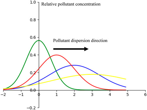
FIGURE 1. Distribution patterns of pollutant concentration at different monitoring cross-sections.

2.2 The construction of optimization model

Using the pollutant dispersion quantification method, the dispersion process of pollutants carried out in the water column is generalized, and the inverse solution of pollutant dispersion using the method of hydrodynamics, the linear correlation between the calculated pollutant concentration c and the observed pollutant concentration C with a correlation coefficient r = 1. The expression of the correlation coefficients,

$r=\frac{{\displaystyle \sum _{i=1}^n}\left(C_i-\overline{C}\right)\left(c_i-\overline{c}\right)}{\sqrt{{\displaystyle \sum _{i=1}^n}{\left(C_i-\overline{C}\right)}^2}\sqrt{{\displaystyle \sum _{i=1}^n}{\left(c_i-\overline{c}\right)}^2}}(8)$

where ‾C and ‾c indicate the arithmetic mean of the observed concentration C and the retrospective concentration c, respectively; n is the value of the observed concentration sequences.

The objective of the optimization model is to find the optimal solution. Although the use of hydraulic transition process can achieve decoupling between the emission location, emission time and emission intensity of the pollutant source, and a series of pollutant emission locations, emission times and emission intensities can be calculated, an optimization algorithm is introduced to find the optimal combination.

Based on the observed concentration sequence C_i, the expression for c_i can be obtained assuming the calculated optimal discharge location X_i and discharge time T_i, and the objective function is constructed as shown in Eq. 12, when and only when X_i = x_i and T_i = t_i, the correlation coefficient r = 1, at which point the objective function reaches the optimal state.

$\min \left(1-r\right),(9)$

2.3 The model construction process

Based on the quantitative positive description of pollutant diffusion, this paper describes the diffusion process of pollutants in the positive direction, and through the analysis of the flow field of the canal, the source term of pollution source is reversed by coupled with the BAS algorithm, which is an optimization calculation that simulates the process of longhorn beetle searching for food. The traditional BAS optimization algorithm adopts the method of fixed step size for optimization calculation, but in the process of traceability, if a fixed step length is used for calculation, it is easy to occur the situation of local optimal solution, which is not conducive to global optimization. In this paper, the BAS algorithm is improved and a method of variable step size is used for optimization calculation to prevent the occurrence of local optimization. The specific steps were as follows:

Step 1:. Obtain the average flow velocity of the river section through monitoring sites.

Step 2:. Through the observation information of the monitoring section of the canal, the equation is constructed according to tequations (2) and (6).

Step 3:. Build a combination of pollution source items (c_i, x_i, t_i).

Step 4:. Determine the objective function of the optimized model (Eqs. 8, 9).

Step 5:. α_l indicates the left whisker position, α_r indicates the right whisker position, o represents the centroid, and d₀ is denoted the distance between the two whiskers. Assuming that the orientation of the ox is arbitrary, then the left/right whiskers of the ox are also arbitrary, normalizing the vector,

$s=\frac{rands\left(m,s\right)}{\parallel rands\left(m,s\right)\parallel }(10)$

where rands (m,s) is the one-dimensional random vector related to the pointing of the longhorn whisker, and m represents the dimension, that is, the number of unknown numbers of the objective function.

Step 6:. After H iterations, the position of the longhorn beetle whiskers can be given by the vector s.

$\left\{\begin{array}{c}{a}_{\mathit{l}}=o_H+\frac{1}{2}{d}_{H}l\\ a_r=o_H+\frac{1}{2}{d}_{H}l\end{array}\right.(11)$

where o_H represents the position of the iteration H subcenter of mass; and d_H represents the distance between the two whiskers of iteration H.

Step 7:. Update the next moment position coordinates of the cattle,

$\begin{array}{c}{a}_H=a_{H-1}+bssign\left[f\left(a_l\right)-f\left(a_r\right)\right]\\ b=c{d}_0\end{array}(12)$

where b is the step size; c is a constant; f (α_l) is the fitness value of α_l, f (α_r) is the fitness value of α_r; sign is a symbolic function. f (α_l)- f (α_r) if positive, indicating that the longhorn is moving to the left; Conversely, it means that the longhorn beetle is moving to the right. For each iteration, the search distance and step size vary as follows,

$\begin{array}{l}{d}_H=\alpha d_{H-1}+d_0\\ b_H=\beta b_{H-1}\end{array}(13)$

where α and β represent the update coefficient of the search distance and the change coefficient of the step size, respectively.

Step 8:. Substitute the a_H obtained in step 7 into the objective function until the optimal solution of the objective function is found or the maximum number of iterations is reached and the iterative calculation is completed.

The flow of the calculation is shown in Figure 2.

FIGURE 2

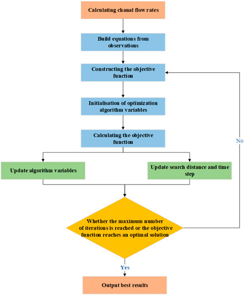
FIGURE 2. Distribution patterns of pollutant concentrations at different monitoring cross-sections.

3 Research cases and discussion

The simulation case assumes the following: the river has a regular rectangular cross-sectional shape with no tributary confluence. The roughness of the river channel was 0.025, the bottom width is 20 m, the water depth is 6 m, the slope drop is 0.0028%, and the longitudinal dispersion coefficient of the river channel was 2.0 m²/s. Assume that 1,000 kg of pollutants are dropped at point A in the middle of 12:00 noon, and the pollutant observation sequence is observed at point B, 5 km downstream from point A, as shown in Figure 3. There will be a water quality testing point every 1 km downstream of point B. The water quality testing point will be monitored every 30 min.

FIGURE 3

FIGURE 3. Observed concentration changed at section B.

3.1 Traceability calculations

According to the average flow velocity of the monitored river channel of about 0.35 m/s, the default pollutant in the process of diffusion of the river channel flow pattern is stable, the flow velocity does not change, the starting time of the calculation from 10: 55, extract the monitoring data of all downstream observation sections, and obtain the retrospective observation series (M₀, M₁, M₂. . . . . . ., M_n), (x₀, x₁, x₂. . . . . . . , x_n), (t₀, t₁, t₂, . . . . . . . , t_n), and a 10% observation error was added to the calculated results to account for instrumental monitoring errors. The source term series was solved iteratively using the BAS optimization algorithm to find its optimal solution. The number of iterations was chosen to be 5000, and the iteration curves for the three parameters are shown in Figure 4.

FIGURE 4

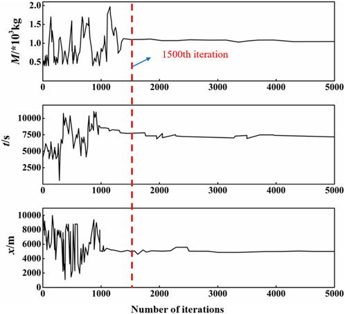
FIGURE 4. Retrospective calculation of iterative curves.

As it can be seen from Figure 4, the pollutant drop quality, drop time and drop location all tend to stabilize after 1500 iterations and stabilize around the true value. For the first 1500 iterations of the calculation, all three source terms produced huge fluctuations due to instability in the calculation of the algorithm during initialization, and these fluctuations were not very helpful for the inversion results. To further prove the reliability of the retrospective calculation results, the results of the first 1500 iterations were excluded and the results of the other 3500 calculations were analyzed, and the analysis results are shown in Table 1.

TABLE 1

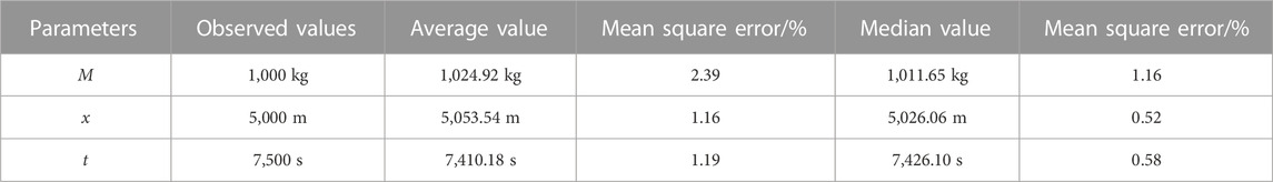
TABLE 1. DP-BAS traceability calculation statistics results.

As can be seen from Table 1, in the process of traceability calculation the overall calculation accuracy is relatively high. Although there is a significant error in calculating the mass M of pollutants, the mean square error is only 2.39%, and the calculation error for the pollutant placement position x is the smallest, with a mean square error of only 1.16%.

As a comparison, DE-MCMC (Shi et al., 2023) and GA method were applied to the traceability calculation of the same scenario, and the calculation results are shown in Table 2 and Table 3.

TABLE 2

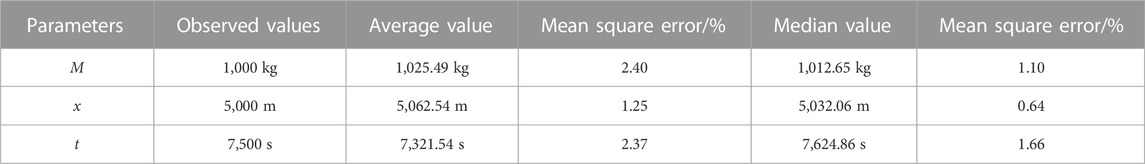
TABLE 2. Statistical results of the DE-MCMC methods.

TABLE 3

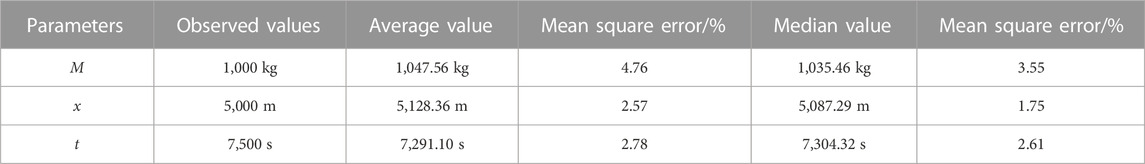
TABLE 3. The GA statistical results.

From Table 2, it can be seen that the traceability method proposed has higher accuracy than the DE-MCMC method in terms of pollutant quality and placement time, and the difference between the results calculated by the DP-BAS and DE-MCMC method is relatively small in terms of pollutant location.

As can be seen from Tables 1–3, the inversion deviation of both the mean and median values of the pollutant source terms using the GA method is greater than that of the DP-BAS method, and the GA method has the worst effect on the inversion of the pollutant quality, with the mean square error of 4.76%, while the mean square error of DP-BAS is 2.39%. Through the three inversion methods, it can be found that the pollutant quality is the worst source term in the inversion processes, with mean square errors of 2.39%, 2.40%, and 4.76%, respectively. This may be due to the fact that in the process of pollutant dispersion, the empirical equations experimentally fitted to the longitudinal dispersion process of pollutants are used in the physical model, so the errors accumulate in the traceability process, resulting in a larger deviation of the pollutant emission quantities compared with the other inversion terms. In order to further compare the above three methods, the maximum, minimum and average errors of the three methods were analyzed, the results of the analysis are shown in Table 4.

TABLE 4

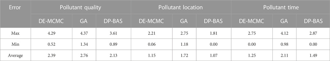
TABLE 4. The error analysis of DE-MCMC, GA and DP-BAS method.

From Table 4 for the quality of pollutant release, the traceability results of DE-MCMC are consistent with the DP-BAS method in this paper. However, for the location and time of pollutant discharge, the results calculated by DP-BAS are better than those obtained using DE-MCMC method. In addition, the DP-BAS method outperforms the traditional GA algorithm in the inversion results of the three source terms of pollutants. Through the comparison of three methods, the inversion results of pollutant emission quality are relatively not well, the average errors of DE-MCMC, GA and DP-BAS are 2.39, 2.76, and 2.13, respectively. Second, the difference between the maximum and minimum errors calculated by DE-MCMC in the three source terms is 3.77, 2.15, and 2.75, respectively. While the difference between the maximum and minimum errors calculated by GA in the three source terms is 3.03, 2.57, and 3.14. The above difference are greater than the results of the proposed the DP-BAS method. In the process of traceability calculation, DP-BAS method can ensure the stability of model calculation and avoid excessive deviation between the simulation and the actual value. Besides, for the DE-MCMC and GA methods, a large number of scholars have confirmed that the two methods have relatively reliable calculation accuracy in traceability, but the traceability method proposed based on velocity dynamic programming also has certain reliability and stability in the identification of pollutant source terms.

There is no need to enter concentration data in the hydrodynamic-water quality model for the difference inverse solution of the St. Venant equation system—convection equation because this study uses the pollutant dispersion quantification method instead of the coupled hydrodynamic-water quality model to calculate the diffusion process of pollutants. Instead optimization algorithms are used to quantify the pollutant instead, the calculation time is shown in Table 5.

TABLE 5

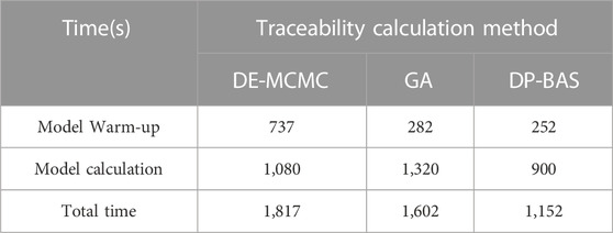
TABLE 5. Comparison of the calculation time of three traceability calculation methods.

As observed in Table 5, the model warm-up period (calculation result oscillation) and the model calculation period make up the entirety of the traceability calculation. The table shows that the model warm-up and calculation times for DP-BAS are less than those for DE-MCMC and GA. This is because DE-MCMC and GA also perform the quadratic differential inverse solution of St. Venant and convective equations. Model warm-up times for GA and DP-BAS algorithms are comparable, while the DE-MCMC technique requires additional error sampling during the inverse solution, which increases warm-up times significantly. Additionally, the method calls for an error sampling calculation, which while somewhat correcting the problem also significantly slows down computation performance. In terms of model calculation time, DP-BAS and DE-MCMC are comparable; DP-BAS benefits from variable step size, so the calculation speed and accuracy are guaranteed in the calculation process; DE-MCMC has already performed the sampling error calculation in the preheat calculation, so the calculation speed and accuracy are also guaranteed in the model calculation; however, GA is constrained by its fixed step size, so the calculation speed and accuracy are only guaranteed in the model calculation. This will considerably lessen the impact of model computation since the local optimum solution will remain emerging while obtaining the global optimal solution, which will then be discovered in the local optimal solution.

Overall, both in terms of model computing speed and actuarial correctness, the DP-BAS in this study offers distinct benefits. In contrast to the conventional optimization algorithm, this paper enhances the optimization algorithm by converting the conventional fixed-step calculation into a variable-step calculation, which simultaneously increases the computational accuracy and speed of the model. The traditional algorithm uses implicit difference to quadratic difference in the St. Venant system of equations-convective equations for forward simulation and backward trace calculation of pollutants, whereas the quantized diffusion equation used in this paper greatly improves the calculation rate.

4 Conclusion

In this paper, the quantitative equation of pollutant diffusion is proposed based on physical model experiments, and the temporal and retrograde traceability of sudden water pollution in river and canal water quality is investigated through the pollutant traceability model of coupled DP-BAS algorithm. The following main conclusions were obtained:

(1) The convective diffusion equation is simplified into a quantitative formula, and a traceability method with the average flow velocity of the river and canal as the main independent variable is proposed through parameter generalization, which is simple and practical.

(2) The DP-BAS method decouples the pollutant diffusion parameters and solves the pollutant concentration, location and time separately, which reduces the solution dimension of traceability and avoids the traditional model falling into the local optimal solution. Thus, the efficient identification of sudden water pollution is possible.

(3) Through this case study, the traceability outcomes and calculation rate of the model are improved. The DE-MCMC and GA techniques were compared and validated, and the results showed that the traceability model has excellent accuracy and dependability.

(4) Although the DP-BAS method reduces the difficulty of the traditional traceability model, in future research, more in-depth studies on the quality of pollutant traceability through more case studies and descriptions of the generalizability of the model are needed.

Data availability statement

The original contributions presented in the study are included in the article/Supplementary Material, further inquiries can be directed to the corresponding authors.

Author contributions

FL and HR: software, methodology, data curation, validation, conceptualization, methodology, writing—original draft, review and editing. YT and NZ: investigation and visualization. YL, RW, and YH: funding acquisition and project administration. All authors contributed to the article and approved the submitted version.

Funding

This work was supported by the National Key Research and Development Program of China (No. 2021YFD2000200); the National Key Research and Development Program of China (No. 2019YFE0125700); the National Key Research and Development Program of China (No. 2018YFC1802700) and the National Natural Science Foundation of China (No. 51809002).

Conflict of interest

The authors declare that the research was conducted in the absence of any commercial or financial relationships that could be construed as a potential conflict of interest.

Publisher’s note

All claims expressed in this article are solely those of the authors and do not necessarily represent those of their affiliated organizations, or those of the publisher, the editors and the reviewers. Any product that may be evaluated in this article, or claim that may be made by its manufacturer, is not guaranteed or endorsed by the publisher.

References

Cao, X. Q., Song, J. Q., Zhang, W. M., and Zhang, L. L. (2010). MCMC method on an inverse problem of source term identification for convection-diffusion equation [J]. J. Hydrodynamics Ser A 25 (2), 127–136. doi:10.3969/j.issn.1000-4874.2010.02.001

CrossRef Full Text | Google Scholar

Charles, L. K., Igor, Y., and Keith, N. (2000). Solving inverse initial-value, boundary-value problems via genetic algorithm. Eng. Appl. Artif. Intell. 13 (6), 625–633. doi:10.1016/s0952-1976(00)00025-7

CrossRef Full Text | Google Scholar

Chen, H. Y., Teng, Y. G., Wang, J. S., Song, L. T., and Zhou, Z. Y. (2012). Event source identification of water pollution based on Bayesian-MCMC[J]. J. Hunan Univ. Nat. Sci. 39 (6), 74–78. doi:10.3969/j.issn.1674-2974.2012.06.014

CrossRef Full Text | Google Scholar

Cheng, W. P., and Jia, Y. (2010). Identification of contaminant point source in surface waters based on backward location probability density function method. Adv. Water Resour. 33 (4), 397–410. doi:10.1016/j.advwatres.2010.01.004

CrossRef Full Text | Google Scholar

Cheng, W. P., and Liao, X. J. (2011). One-dimensional pollution source emission reconstruction based on inverse probability density function[J]. J. Hydrodynamics Ser A 26 (4), 460–469. doi:10.3969/j.issn1000-4874.2011.04.010

CrossRef Full Text | Google Scholar

Dooge, J., and Bruen, M. (2005). Problems in reverse routing. Acta Geophys. Pol. 53 (4), 357–371. doi:10.1007/978-3-319-05035-5_4

CrossRef Full Text | Google Scholar

Ghane, A., Mazaheri, M., and Samani, J. M. V. (2016). Location and release time identification of pollution point source in river networks based on the Backward Probability Method. J. Environ. Manag. 180, 164–171. doi:10.1016/j.jenvman.2016.05.015

CrossRef Full Text | Google Scholar

Gorelick, S. M., Evans, B., and Remson, I. (1983). Identifying sources of groundwater pollution: An optimization approach. Water Resour. Res. 19 (3), 779–790. doi:10.1029/wr019i003p00779

CrossRef Full Text | Google Scholar

Han, K., Zuo, R., Ni, P., Xue, Z., Xu, D., Wang, J., et al. (2020). Application of a genetic algorithm to groundwater pollution source identification. J. Hydrology 589, 125343. doi:10.1016/j.jhydrol.2020.125343

CrossRef Full Text | Google Scholar

Jha, M., and Dattb, B. (2012). Three-dimensional groundwater contamination source identification using adaptive simulated annealing. J. Hydrologic Eng. 18 (3), 307–317. doi:10.1061/(asce)he.1943-5584.0000624

CrossRef Full Text | Google Scholar

Kanao, S., and Sato, T. (2022). Numerical estimation of multiple leakage positions of a marine pollutant using the adjoint marginal sensitivity method. Comput. Fluids[J]. 232, 105195. doi:10.1016/j.compfluid.2021.105195

CrossRef Full Text | Google Scholar

Kong, Y., He, W. J., Shen, J. Q., Yuan, L., Gao, X., Ramsey, T. S., et al. (2023). Adaptability analysis of water pollution and advanced industrial structure in Jiangsu Province, China. Ecol. Modell. 481, 110365. doi:10.1016/j.ecolmodel.2023.110365

CrossRef Full Text | Google Scholar

Lei, F., Ou, J., Wang, X., and Zhu, H. (2022). Radial basis collocation method with parameters optimized for estimating pollutant release history. Environ. Sci. Pollut. Res. 29 (13), 19847–19859. doi:10.1007/s11356-021-17144-8

CrossRef Full Text | Google Scholar

Long, Y., Xu, G. B., Ma, C., and Chen, L. (2016) Emergency control system based on the analytical hierarchy process and coordinated development degree model for sudden water pollution accidents in the Middle Route of the South-to-North Water Transfer Project in China. Environ. Sci. Pollut. Res. 26(12), 12332–12342. doi:10.1007/s11356-016-6448-0

CrossRef Full Text | Google Scholar

Long, Y., Xu, G., and Ma, C. (2017). Pollutant transport rules under synchronous control and asynchronous control[J]. Chin. J. Environ. Eng. 11 (2), 709–714. doi:10.12030/j.cjee.201509162

CrossRef Full Text | Google Scholar

Mou, X. Y. (2011). Research on inverse problem of pollution source term identification based on differential evolution algorithm[J]. J. Hydrodynamics Ser A 26 (1), 24–30. doi:10.3969/j.issn1000-4874.2011.01.004

CrossRef Full Text | Google Scholar

Najafzadeh, M., Noori, R., Afroozi, D., Ghiasi, B., Hosseini-Moghari, S. M., Mirchi, A., et al. (2021). A comprehensive uncertainty analysis of model-estimated longitudinal and lateral dispersion coefficients in open channels[J]. J. Hydrology 603 (9), 1879–2707. doi:10.1016/j.jhydrol.2021.126850

CrossRef Full Text | Google Scholar

Neupaue, R. R. M., and Wilson, J. L. (2001). Adjoint-derived location and travel time probabilities for a multidimensional groundwater system. Water Resour. Res. 37 (6), 1657–1668. doi:10.1029/2000wr900388

CrossRef Full Text | Google Scholar

Shang, T. (2012). Research on water pollution source tracing method based on GIS-A case study of dahuofang reservoir[D]. Shenyang: Shenyang Jianzhu University.

Google Scholar

Shi, P. F., Yang, T., Yong, B., Xu, C. Y., Li, Z., Wang, X. Y., et al. (2023). Some statistical inferences of parameter in MCMC approach and the application in uncertainty analysis of hydrological simulation[J]. J. Hydrology 617, 12. doi:10.1016/j.jhydrol.2022.128767

CrossRef Full Text | Google Scholar

Sullivan, C. A., Meigh, J. R., and Giacomello, A. M. (2003). The water poverty index: Development and application at the community scale. Nat. Resour. Forum 27 (3), 189–199. doi:10.1111/1477-8947.00054

CrossRef Full Text | Google Scholar

Sun, D., Liu, X., Long, X., and Zhang, C. (2020). Spatial and temporal heterogeneity of water poverty in China: Based on WPI model(in Chinese)[J]. J. Of Nanjing Tech Univ. 19 (5), 104–114.

Google Scholar

Wang, J. B., Lei, X. H., Liao, W. H., and Wang, H. (2015). Source identification for river sudden water contamination based on coupled probability density function method[J]. J. Hydraulic Eng. 46 (11), 1280–1289. doi:10.13243/j.cnki.slxb.20150405

CrossRef Full Text | Google Scholar

Xin, X. K., Han, X. b., Li, J., and Lu, L. (2014). Pollutant source identification model of water pollution incident based on genetic algorithm[J]. Water Resour. Power 32 (7), 52–55.

Google Scholar

Yan, X., Dong, W., An, Y., and Lu, W. (2019). A Bayesian-based integrated approach for identifying groundwater contamination sources. J. Hydrology 579, 124160. doi:10.1016/j.jhydrol.2019.124160

CrossRef Full Text | Google Scholar

Yang, H. D., Xiao, Y., Wang, Z. M., Shao, D. G., and Liu, B. Y. (2014). Traceability method of sudden water pollution incident[J]. Adv. Water Sci. 25 (1), 122–129. doi:10.14042/j.cnki.32.1309.2014.01.012

CrossRef Full Text | Google Scholar

Yuan, F., Liu, Y. H., and Guo, J. Q. (2017). Simplex-particle swarm algorithm for parameter estimation in two-dimensional water quality model of river[J]. South-to-North Water Transfers Water Sci. Technol. 15 (04), 193–197+202. doi:10.13476/j.cnki.nsbdqk.2017.04.031

CrossRef Full Text | Google Scholar

Yuan, L., Ding, L. W., He, W. K., Kong, Y., Ramsey, T. S., Degefu, D. M., et al. (2023). Compilation of water resource balance sheets under unified accounting of water quantity and quality, a case study of Hubei province. [J].Water. 15 (7), 1383. doi:10.3390/w15071383

CrossRef Full Text | Google Scholar

Yuan, L., Yang, D. Q., Wu, X., He, W. J., Kong, Y., Ramsey, T. S., et al. (2023). Development of multidimensional water poverty in the Yangtze River Economic Belt, China. J. Of Environ. Manag. 324, 116608. doi:10.1016/j.jenvman.2022.116608

CrossRef Full Text | Google Scholar

Zhang, F., Wang, W. L., and Cheng, J. M. (2010). Emergency system conception of sudden water pollution accident in river basin[J]. Environ. Sci. Technol. 23 (1), 57–60. doi:10.1021/acs.est.9b01024

CrossRef Full Text | Google Scholar

Zhong, A. J., Li, L., Zhang, L., Zhong, X. Y., and Shi, L. S. (2005). Digital water environment management system and digital water quality early warning forecast system integration[J]. China rural water and hydropower 12, 20–22.

Google Scholar

Zhu, J. (2014). Study on traceability of sudden water pollution based on mobile platform[D]. Hangzhou: Zhejiang University.

Google Scholar