Historical global and regional spatiotemporal patterns in daily temperature

1 Introduction

Many lines of evidence suggest that globally-averaged surface air temperature has increased over the last several decades. However, many details about the spatio-seasonal properties of these trends remain unknown, either because recent such studies focus on the local to regional scale, such as for China (Yiqi et al., 2023) and Latvia (Kalvāns et al., 2023), or even the hemispheric scale (Deng and Fu, 2023), or because global-scale studies tend to examine annual trends (e.g., Lindsey and Dahlma, 2020). Distribution within the day-night cycle of that long-term temperature trend has remained uncharacterized holistically using long-term, high-resolution data collected within the Satellite Era.

The objective of this manuscript is to examine the global trend using a current reanalysis data set and then to elucidate the regionality of the daily temperature trends by month across the terrestrial Earth. To identify whether the method of calculating the daily trend influences the results, we calculate daily means by averaging the daily maximum and minimum values, and also by considering “daily” as the mean of the 24 hourly values. This approach will strengthen our knowledge of the extent to which nuances in the calculation method influence the regionality and monthly distribution of the temperature trends.

Four hypotheses regarding the daily mean surface air temperature over the terrestrial Earth are tested. The first is that the method of calculating daily mean temperature (i.e., “meanmaxmin” vs. “meanhourly”) produces statistically significantly different temperatures. Testing this hypothesis is important because it has long been recognized that maximum and minimum temperatures change asymmetrically, with minimum temperature often changing more substantially than the maximum (Karl et al., 1993). The next two are that a linear temporal trend exists in the global annual mean temperature, and in the global monthly mean temperatures for each of the 12 months, for the Earth as a whole. These hypotheses are important to test again for the post-Satellite Era, now that more updated data and data sets are available. The fourth hypothesis is inspired by the comments of Michaels and Stooksbury (1992) about the importance of the regionality and seasonality of the warming; we hypothesize that the temporal trend is not uniform spatially by month.

2 Background

A rapid increase in research on the globally increasing trend in observed surface air temperature had begun by the latter part of the 20th century. For example, after correcting for inconsistencies in the temperature record due to instrumental inaccuracies, non-uniform measurement techniques, changes in spatial coverage, and irregularity in time and location of the measurements, Jones et al. (1986) detected a long-term warming trend at a monthly scale from 1861 to 1984, with the three warmest years in the 1980s. In an analysis of annual time series from 1854 to 1988, Ghil and Vautard (1991) found an insignificant surface air temperature trend until 1910 and an increase of 0.4C° afterwards, with some inter-annual and inter-decadal oscillations due to the El Niño-Southern Oscillation (ENSO) phenomenon (Rasmusson et al., 1990) and extratropical ocean circulation (Bjerknes, 1964). Liebmann et al. (2010) identified a similar trend over the 1850 to 2009 time series.

With the availability of 30 years of air temperature data measured during the Satellite Era came more robust and precise global temperature climatologies. For example, in examining global temperature data from 1979 to 2010 from surface and satellite records, Foster and Rahmstorf (2011) found steady statistically significant warming trends ranging from 0.014 to 0.018°C per year for five global data sets, after discarding short-term variability, with the warmest 2 years at the end of the data series. Several studies during this era offered suggestions for attribution, including predominantly anthropogenic (Lean and Rind, 2008), anthropogenic with some impact of solar forcing (Wild et al., 2007), multidecadal variability associated with strengthening of the global thermohaline circulation and some impact from greenhouse gas accumulation (Wu et al., 2007; Wu et al., 2011), sea surface temperatures associated particularly with the Pacific decadal variability pattern (Wang et al., 2009), the Atlantic meridional overturning circulation (Keenlyside et al., 2008; Semenov et al., 2010; DelSole et al., 2011), and a combination of the above effects (Swanson et al., 2009).

The increasing availability of high-resolution observational and proxy and climate model output further enhanced global air temperature trend analysis spatially and temporally. For example, Marcott et al. (2013) quantified the global temperature trends since the last deglaciation, including the relatively warm mid-Holocene, subsequent cooling of approximately 0.7°C over the next 5,000 years into the Little Ice Age, and abrupt and steady warming since that time, with a global mean temperature today exceeding that during 90 percent of the Holocene. Marotzke and Forster (2015) identified discrepancies between the climate model output, which showed a significant long-term temperature increase from 1900 to 2012, and the observational data, which includes a hiatus in the increasing trend. Using a combination of observations, global climate model simulations, and proxy evidence, Hawkins et al. (2017) found that 1986–2005 was likely 0.55–0.80°C warmer globally than preindustrial times. Variability of temperature about the long-term warming trend has also been a focus area in recent years. Climate model ensembles suggest that equilibrium climate sensitivity (ECS), defined as the change in temperature after atmospheric CO₂ instantly doubles and equilibrium is reached (Meraner et al., 2013), is between 2.3 and 4.7°C at a 95% confidence interval (Sherwood et al., 2020), with a central estimate at 2.8°C (Cox et al., 2018), but possibly even greater (Zelinka et al., 2020), though Scafetta (2022) suggested that it could be lower. In addition to evaluating the increasing global temperature trend, climate modeling has projected future air temperature trends under different climate scenarios (Collins et al., 2013). Similarly, many analyses of terrestrial surface air temperature have been conducted in the last few years (e.g., Toreti and Desiato, 2008; You et al., 2010; Jain & Kumar, 2012; Saboohi et al., 2012; Ji et al., 2014; Sato and Robeson, 2014; Deniz and Gönençgil, 2015; Dong et al., 2015; Gonzalez-Hidalgo et al., 2015; Mondal et al., 2015; Chattopadhyay and Edwards, 2016; Ahmadi et al., 2018; Asfaw et al., 2018; Ghasemifar et al., 2020; Matewos and Tefera, 2020; Miheretu, 2021), but of these, only Ji et al. (2014) worked at the global scale. While many other studies (e.g., Intergovernmental Panel on Climate Change, (2021) and the many references contained within it) assert that the near-surface atmosphere is warming, few recent studies consider the details of the spatial distribution of that warming globally, at fine spatio-temporal resolution.

Models have generated data sets that have been used to analyze temperature and other variables globally. Much of this work has used the first-generation National Center for Atmospheric Research Reanalysis product (Kalnay et al., 1996). More recent efforts have used the second generation products (Kanamitsu et al., 2002), which improved the spatial resolution from 5° to 2.5° for results since the Satellite Era began in 1979. Data sets with much greater spatial resolution have also been developed based on interpolation techniques. Hijmans et al. (2005) produced an impressive early data set available at 1-km resolution, for the terrestrial Earth. The National Centers for Environmental Prediction (NCEP) developed the NCEP Climate Forecast System Reanalysis (CFSR) to emphasize the coupled atmosphere-ocean-land surface-sea ice system, at 38-km spatial resolution and 64 atm levels, with 40 levels at resolution of 0.5° or finer (Saha et al., 2010). NASA’s Famine Early Warning Systems Network (FEWS NET) Land Data Assimilation System (FLDAS; McNally et al., 2017) is available at a spatial resolution of 0.1 × 0.1 from 1982 to present. Other highly respected data sets include ECOCLIMAP-V1 (Masson et al., 2003), Global Precipitation Climatology Centre (Schneider et al., 2017), WorldClim 2.0 (Fick and Hijmans, 2017), and ENACTS (International Research Institute for Climate and Society, 2017). The Japanese 55-year Reanalysis Project (JRA-55; Japan Meteorological Agency, 2014) has also been important for understanding historical temperature trends globally. Rohli et al. (2019) summarized several key features of JRA-55, as described by Kobayashi (2016), including: 1) length and completeness of the time series for full observing system reanalysis using the most advanced data assimilation scheme, 2) incorporation of several new observational data sets, 3) introduction of a new radiation scheme, 4) improvements offered by variational bias correction over the previous iteration (JRA-25), and 5) availability of companion data sets that permit the assessment of the impact of data assimilation.

A recent addition to the global reanalysis data sets is the European Centre for Medium-range Weather Forecasts (ECMWF) Reanalysis Version 5 (ERA5; Copernicus Climate Change Service (C3S), 2019). ERA5 provides benefits that originated in its predecessor (ERA-Interim reanalysis; Dee et al., 2011) which include improved model physics, core dynamics, and data assimilation (Hersbach et al., 2020). This data set has already been used in a wide range of atmospheric and environmental research. Recent studies have reported that ERA5 generally corresponds well to surface temperature observations in East Africa (Gleixner et al., 2020) and Antarctica (Zhu et al., 2021). Yang et al. (2022) found overall improved performance for ERA5 and 20th Century Reanalysis version 3 (20CRv3; Slivinski et al., 2019) over other reanalysis data sets. Of course, it should be remembered that these reanalysis data sets, including the ERA5, are indeed model output themselves, drawn from a wide array of input data.

3 Materials and methods

Hourly air temperature at 2 m above the terrestrial surface is collected from the ERA5 output for the period 1 January 1981 to 31 December 2020, at a resolution of 0.1 × 0.1 (or approximately 11.1 km at the equator). This data set is compiled from NetCDF files, resulting in an array of 365.25 × 24 × 40 temperature values for each of the 2,212,863 grid points located over land. The mean daily temperature is then calculated, by grid point, in two separate ways: first, as the mean of the maximum and minimum values on a calendar day (“meanmaxmin”), and second, as the mean of the 24 hourly observations (“meanhourly”). The time series of monthly mean global temperatures, calculated from the daily means, is then computed using both the meanmaxmin and meanhourly approaches. A statistically significant difference in the temperature distributions indicates that both approaches should be used in testing the hypotheses.

Differences in local time infer that the daily temperature value for a given calendar day at a given grid point is actually based partially on values for the calendar day before or after the reported value, except for grid points within the Greenwich mean time zone. Increasing offset from Greenwich mean time corresponds to less overlap of the hourly, and therefore daily, meanmaxmin, and meanhourly values with that of the calendar day. No adjustment is made for this inconsistency, as it creates no complication for the hypothesis testing.

Testing of each hypothesis requires investigation of linear temporal trends. To avoid relying on assumptions of normality of the distribution, serial independence, and long time series, non-parametric tests of serial randomness in the form of rank correlation methods are appropriate and robust (Mitchell et al., 1966). The Mann-Kendall test (Mann, 1945; Kendall, 1948; Kendall, 1995) and the synonymous (Qian et al., 2015) Şen’s estimator method (P.K. Şen, 1968; Z. Şen, 2012; 2014) have been useful for identifying the statistical significance of a linear trend in similar research (e.g., Mondal et al., 2012; Mahmood et al., 2019; Panda and Sahu, 2019; Sayyad et al., 2019; Yacoub and Tayfur, 2019; Alemu and Dioha, 2020; Bojago and YaYa, 2021; Chand et al., 2021). Likewise, Spearman’s rank-order test for trend (Mitchell et al., 1966) is also widely used in similar work (Rahman et al., 2017), including on temperature trends (e.g., Yücel et al., 2019; Singh et al., 2021). Serra et al. (2001) noted that Spearman is generally more appropriate for large sample sizes with few tied ranks (although Mitchell et al. (1966) suggested that Spearman is more appropriate for handling tied ranks), and for data sets with non-monotonic trends (i.e., with multiple inflection points) in which the focus is on long-term trends rather than abrupt changes. Thus, the Spearman test is selected here over the Mann-Kendall test, but several time-series analyses in geophysical data sets (e.g., Yue et al., 2002; Kahya and Kalaycı, 2004; Rahman et al., 2017) have shown little difference in the results and power, defined as the probability of correctly rejecting a false null hypothesis (Villarini et al., 2009) in the two tests. Levels of significance of 0.05 and 0.10 are used to represent statistical significance for all trends.

In testing the first two hypotheses, if daily temperature from the 2,212,863 terrestrial grid points were simply averaged into a single global value for each calendar day, the convergence of meridians of longitude poleward would cause the 0.1°-spaced meridians to oversample the polar areas relative to the low latitudes. Thus, calculation of the global mean temperature annually and for each month (using both the meanmaxmin and meanhourly methods, separately) contains an extra step. Specifically, the mean terrestrial latitudinal temperature (${\overline{T}}_i$), where $i$ represents the latitude at 0.1° increments over the terrestrial Earth (i.e., from the South Pole (90°S) to 83.5°N), is multiplied by the cosine of its latitude, at each of the 0.1°-spaced parallels (separately). Then, these values are divided by the sum of the cosines of the latitudes to compute the global mean terrestrial temperature for that Julian day (${\overline{T}}_G$) adjusted for the convergence of longitudes at the poles. Thus,

${\overline{T}}_G=\frac{{\displaystyle {\sum }_{-90}^{83.5}}\left({\overline{T}}_i\cos i\right)}{{\displaystyle {\sum }_{-90}^{83.5}}\left(\cos i\right)}$

Monthly aggregated maps comprised of averages of each of the ${\overline{T}}_G$ maps from that month, across the time series are shown here. In other work not shown here, the set of daily maps can be used to identify trends in finer detail.

The daily meanmaxmin- and meanhourly-adjusted ${\overline{T}}_G$ values are compared statistically (Hypothesis 1). The annual (Hypothesis 2) and monthly (Hypothesis 3) global terrestrial temperatures are then calculated for the two approaches. Thus, all 365 of the ${\overline{T}}_G$ values for a given calendar year (discarding leap days) are aggregated for a single annual global temperature (Hypothesis 2), and all 28, 30, or 31 ${\overline{T}}_G$ values for that month in a given calendar year are aggregated for a single monthly global temperature, for each of the 12 months (Hypothesis 3). Spearman tests for trend are run on the 40 data points (i.e., one data point per year) (Hypothesis 2), and for each of the 12 months of the year (Hypothesis 3).

For addressing the “regionality” component of Hypothesis 4, global terrestrial maps—one for each calendar month using the meanmaxmin and/or meanhourly approach—are produced. Maps for January, April, July, and October are shown here to represent the four meteorological seasons (Trenberth, 1983). Maps showing the Theil-Sen slope (°C yr^-1), areas with p-values surpassing the significance threshold, and temperature (°C) difference (2011–2020 mean minus 1981–1990 mean) are shown. For each grid point, the values are calculated based on the 365 × 40 daily mean values compiled from the hourly values. No temperature correction is necessary for these collections of point-specific calculations. The “seasonality” component of Hypothesis 4 is also assessed cartographically.

4 Results and discussion

Testing Hypothesis 1—that the meanmaxmin and meanhourly calculations yield different results—requires the non-parametric Wilcoxon signed rank test, because the time series of mean monthly temperatures compiled from both approaches are found to be distributed non-normally. Wilcoxon testing reveals that globally, the meanmaxmin temperature significantly exceeds the meanhourly temperature (p-value <<0.05), with a mean difference of 0.20°C. This result aligns with those of Weiss and Hays (2005), who found similar differences between means produced by these two methods. Global mean differences between the two algorithms by month are shown in Table 1.

TABLE 1

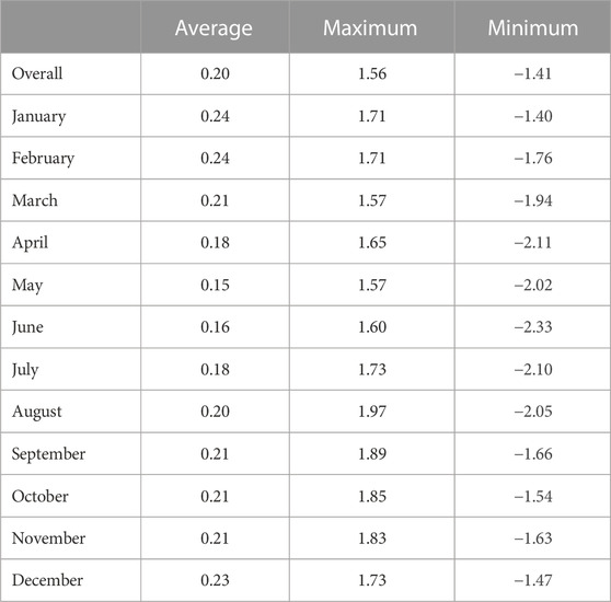
TABLE 1. Globally-weighted mean daily temperature difference (°C), and absolute maximum and minimum temperature difference by gridpoint, by temperature-calculating algorithm (i.e., “meanmaxmin” minus “meanhourly”) by month, 1981–2020.

Moreover, the temperature differences as calculated by the two algorithms vary spatially, as was also found by Weiss and Hays. In most of the world, particularly the Americas and equatorial Africa, the meanmaxmin approach yields the higher temperatures, while in most of northern Africa, the Arabian Peninsula, and central Asia, the opposite is true. Nevertheless, the most extreme difference in the mean temperature calculation at individual places is less than 0.2°C (Figure 1).

FIGURE 1

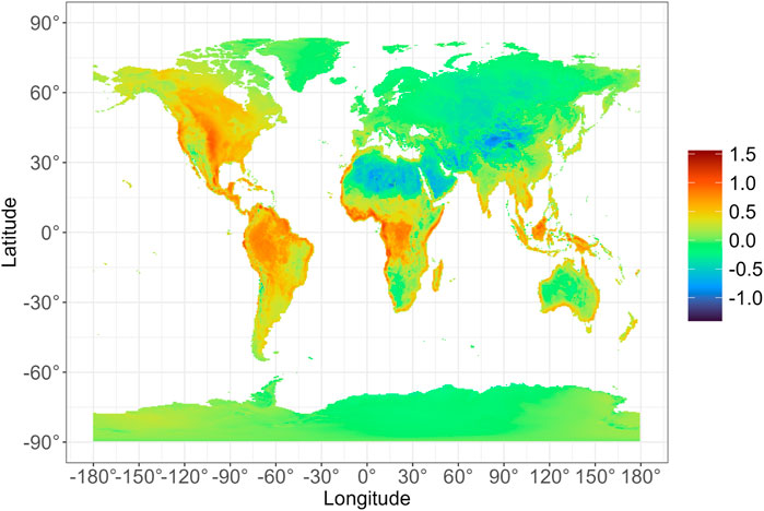
FIGURE 1. Spatial distribution of the daily mean temperature (°C) difference (meanmaxmin minus meanhourly), 1981–2020.

Figure 2 shows these differences using January, April, July, and October as representative of the four seasons, and Supplementary Figure S1 shows the differences for the remaining 8 months. The meanmaxmin-calculated temperature exceeds meanhourly by the greatest amounts in the Americas in April (Figure 2B), and equatorial Africa in April and July (Figures 2B,C), while meanhourly exceeds meanmaxmin in much of northern Africa and Eurasia throughout the year (Figure 2 and Supplementary Figure S1).

FIGURE 2

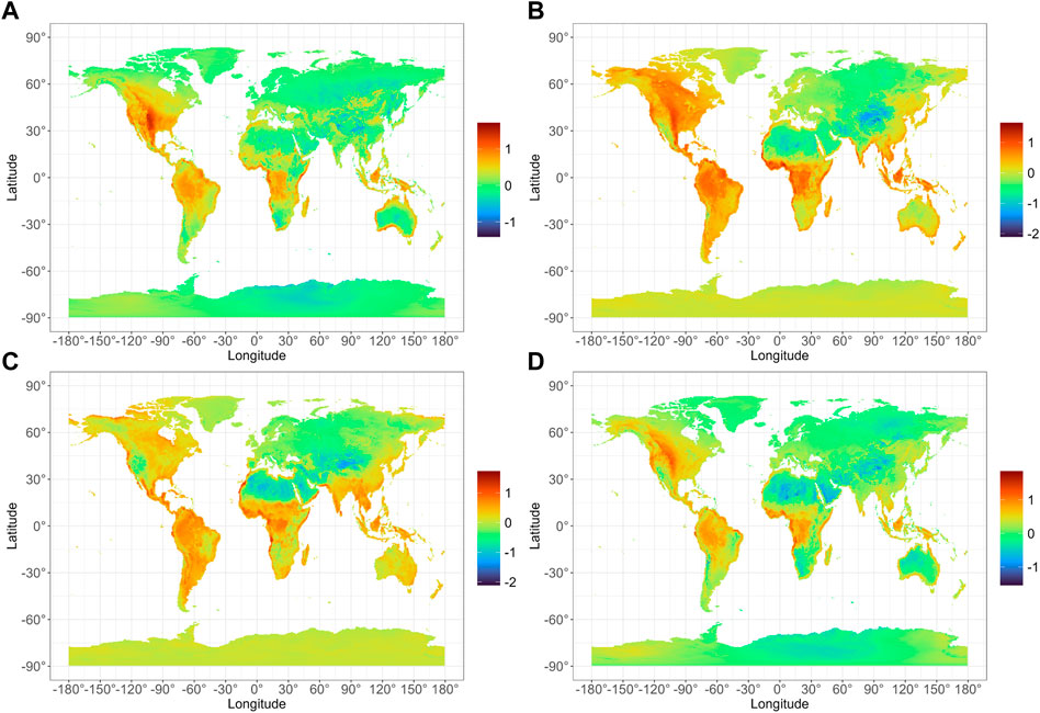
FIGURE 2. As in Figure 1, except for January (A), April (B), July (C), and October (D), over the 1981–2020 period.

Testing of Hypothesis 2 reveals that regardless of whether the meanmaxmin or meanhourly approach is used a linearly increasing trend (Spearman r of 0.861 (p << 0.001) and 0.866 (p << 0.001)) exists in the air temperatures. Hypothesis 3 is confirmed, with the Spearman tests revealing statistically significantly increasing trends (p << 0.001) in each of the 12 months, regardless of whether the meanmaxmin or meanhourly approach is used. The Theil-Şen slope (Akritas et al., 1995) suggests that the rate of temperature increase ranges from 0.022°C yr⁻¹ (August) to 0.033°C yr⁻¹ (October), as shown in (Table 2).

TABLE 2

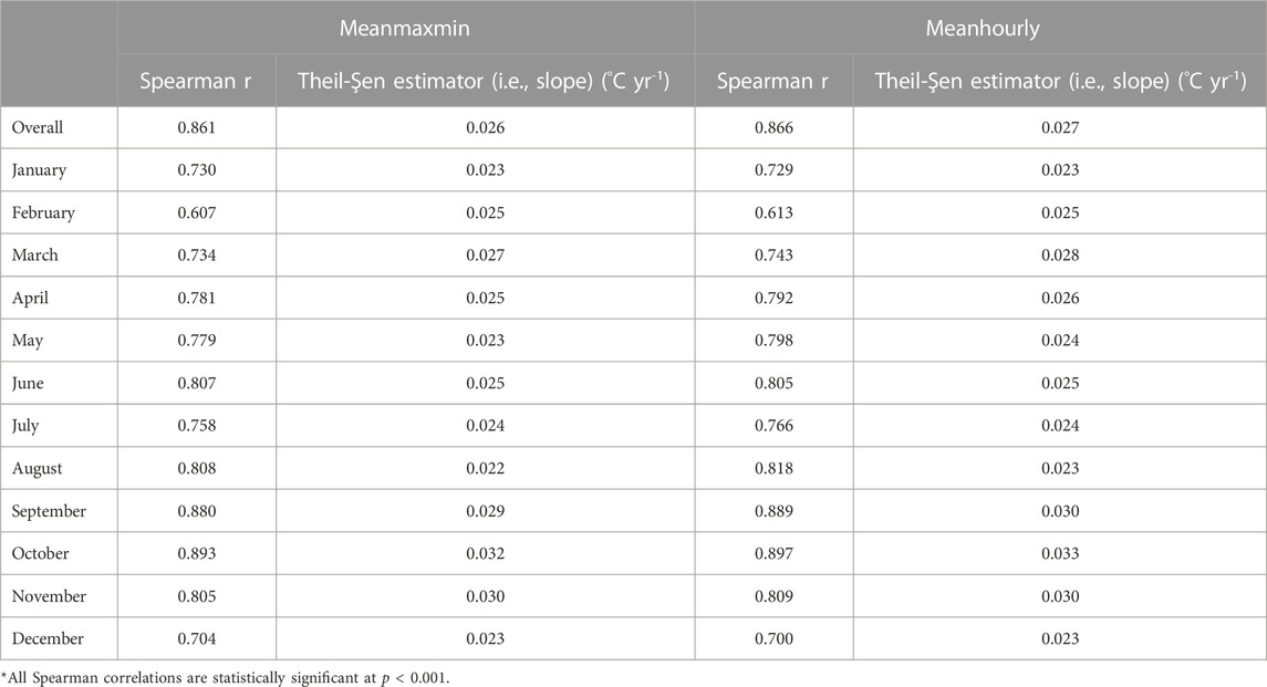
TABLE 2. Spearman correlations and corresponding Theil-Şen slopes for each of the methods of calculating global temporal trends in surface air temperature, 1981–2020.

Regarding the “regionality” aspect of Hypothesis 4, spatial distributions of the rate of annual temperature increase (°C yr⁻¹), as evidenced by the Theil-Şen slope, level of significance, and the absolute temperature increase from the 1981–1990 mean to 2011–2020 mean, are shown in Figure 3, for the meanmaxmin and meanhourly calculations in a side-by-side comparison. Nearly identical results appear for the two approaches, despite previous evidence for the influence of air mass type on the shape of the daily temperature curve (Bernhardt, 2020). Most of the terrestrial Earth is warming at a rate exceeding 0.05°C yr⁻¹ with the steepest rates approaching 0.15°C yr⁻¹ in the Arctic (Figures 3A,B). Some areas, such as Antarctica, the Indian Subcontinent, inland northern North America, and northern Australia, are cooling, but mostly at rates of 0.05°C yr⁻¹ or less (Figures 3A,B). Most of the warming is statistically significant, while nearly all cooling is statistically insignificant (Figures 3C,D). Regardless, however, the absolute value of the temperature change from the 1981–1990 mean to the 2011–2020 mean is less than 2°C (Figures 3E,F).

FIGURE 3

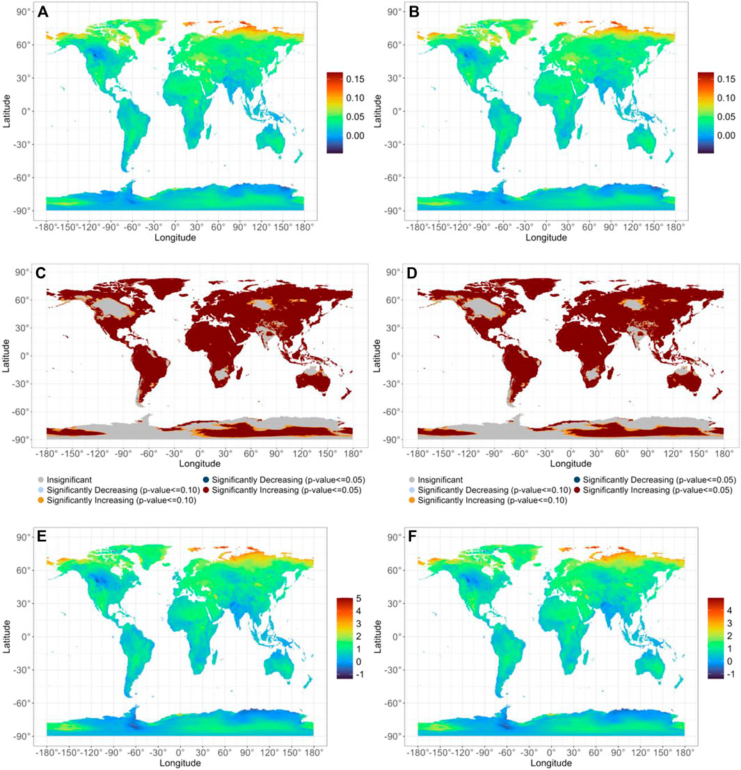
FIGURE 3. Surface air temperature trends (A,B) using the Theil-Şen slope (°C yr^-1), statistical significance at p ≤ 0.05 (C,D), and temperature (°C) difference (2011–2020 mean minus 1981–1990 mean (E,F)), for meanmaxmin (A,C,E) and meanhourly (b, d, and (F) approaches.

Because the spatial patterns shown in Figure 3 are virtually identical for the two methods, results for the “seasonality” component of Hypothesis 4 are shown only for the “meanhourly” approach. Figures 4A–D shows the spatial distribution of the Theil-Şen slope (°C yr⁻¹) for January, April, July, and October, respectively, and those for the remaining months are shown in Supplementary Figure S2. The spatial distribution of statistical significance for those same 4 months across space is shown in Figures 5A–D, with that for the other 8 months shown in Supplementary Figure S3.

FIGURE 4

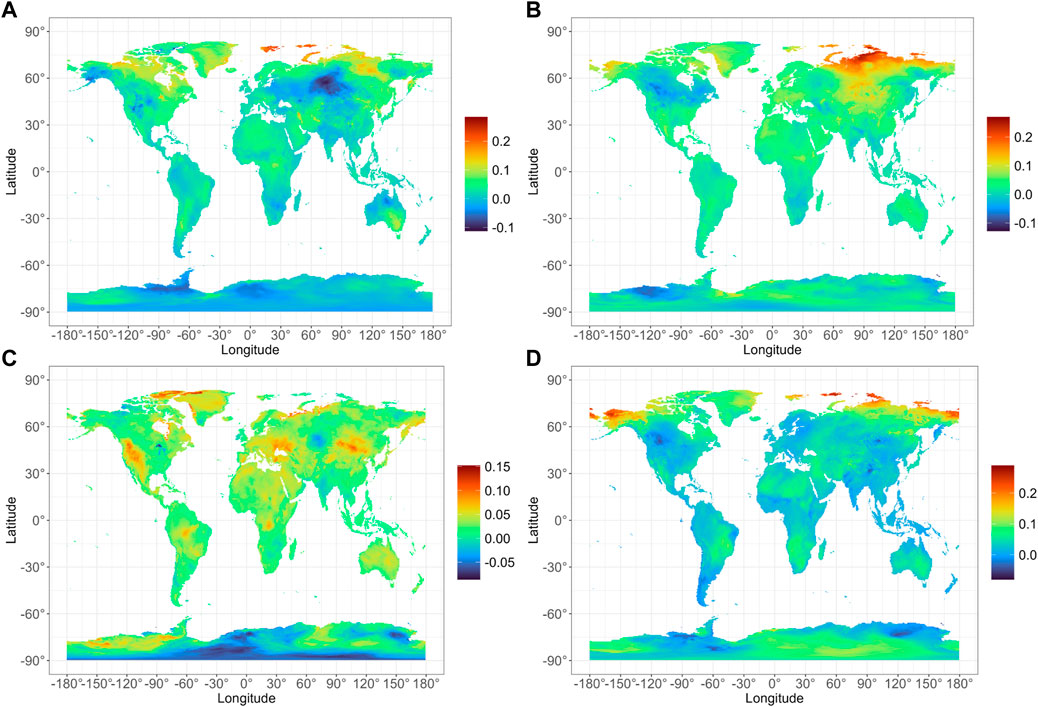
FIGURE 4. Rate of surface air temperature increase using the Theil-Şen slope (°C yr^-1), for January (A), April (B), July (C), and October (D), over the 1981–2020 period, using the “meanhourly” approach.

FIGURE 5

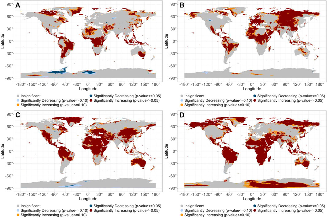
FIGURE 5. Statistical significance (p < 0.05) of Theil-Şen slope shown in Figure 2, for January (A), April (B), July (C), and October (D), over the 1981–2020 period, using the “meanhourly” approach.

The spatial pattern of the temperature rate increase and significance of the temperature trends are similar to the overall patterns shown in Figures 3A–D, but with some additional, notable, monthly features. For instance, the Arctic warming rate is most prominently significant in the transition seasons (Figures 4B,D; Figures 5B,D, and Supplementary Figures S2B–D, F,G, Supplementary Figures S3B–D, F,G), with Arctic cooling prominent in eastern Siberia in February (Supplementary Figure S2A) though not as significant (Supplementary Figure S3A), and in northern North America in February and March (Supplementary Figures S2A,B) though again largely insignificant (Supplementary Figures S3A,B). In the Northern Hemisphere mid-latitudes, warming is most intense in July (Figure 4C and 5C) but not as prominent in the rest of summer (Supplementary Figures S2D,E, S3D,E). Other large, contiguous areas of statistically significant warming trends are in Eurasia in spring, Europe and the lower latitudes in summer, and the tropics in autumn (Figure 4, 5 and Supplementary Figures S2, S3). While data are sparse over the oceans, evidence from island stations indicates that significantly increasing trends also appear in the major ocean basins (Figure 4, 5).

The region of greatest decreasing temperatures is in Antarctica in summer and winter, by approximately 0.1°C yr⁻¹ (Figures 4A,C, and Supplementary Figure S2) but these trends are largely statistically insignificant (Figures 5A,C and Supplementary Figure S3). Other largely statistically insignificant areas of cooling are concentrated over Eurasia in December and January, with some areas of cooling in southwest Asia in November.

The temperature change between the 1981–1990 and 2011–2020 means for January, April, July, and October is shown in Figure 6, with that for the other 8 months shown in Supplementary Figure S4. Again, the strongest warming appears over Arctic Asia, particularly in boreal spring, but with warming in extensive parts of Eurasia, Africa, and the Americas in boreal summer. Cooling appears most substantially in boreal spring in North America and Antarctica, and in boreal autumn in the Americas and much of Eurasia, Africa, and Antarctica, but again, these cooling trends are less substantial than the warming trends.

FIGURE 6

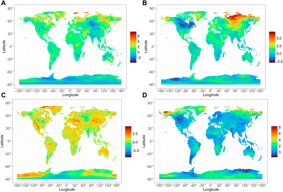
FIGURE 6. Temperature (°C) difference (2011–2020 mean minus 1981–1990 mean), for January (A), April (B), July (C), and October (D)), using the “meanhourly” approach.

The globally-weighted terrestrial air temperature increases between the two averaging periods (1981–1990 vs. 2011–2020) for the meanhourly algorithm is 0.72°C by month. Scafetta (2022) found a 0.58°C increase globally (including oceans) for the 1980–1990 vs. 2011–2021 averaging periods using ERA5 data and reported similar differences using other datasets. For instance, use of UK Met Office Hadley Centre/Climatic Research Unit version 5.0.1.0 (HadCRUT5; Morice et al., 2021) revealed a difference of 0.58°C, and differences of 0.57°C, 0.52°C, 0.52°C, 0.59°C, and 0.56°C were observed using GISTEMP v4 (Lenssen et al., 2019), NOAAGlobalTemp v5 (Huang et al., 2020), HadCRUT4 (Morice et al., 2012), Berkeley Earth group (Rohde and Hausfather, 2020), and Japanese Meteorological Agency (Ishihara, 2006), respectively. A comparison of these results with ours suggests that the terrestrial Earth warmed more than the marine world.

Table 3 shows that the 2011–2020 period is warmer than the 1981–1990 decade in every month, on a globally-weighted average basis, with the greatest warming globally between the two averaging periods in October, followed by September and November, and the smallest increases in December and January. The reduced amount of warming in boreal winter is likely influenced by the lack of ice-albedo effect in the low latitudes, which occupies a large component of Earth’s surface area.

TABLE 3

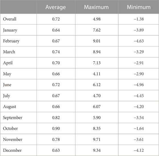
TABLE 3. Globally-weighted difference of means (°C) between the daily mean temperature for the 1981–1990 vs. 2011–2020 averaging periods, using the “meanhourly” algorithm, by month, with absolute maximum and minimum differences at individual grid points.

5 Summary and conclusion

All too often, scientists and the lay public are more concerned with how much the world will warm rather than how it will warm. This research characterized the warming in terms of the geographical distribution and its seasonality, using recently-available, high-resolution ERA5 temperatures, synthesized from a wide array of data sources, and with the daily mean temperature calculated as the mean of the daily maximum and minimum temperature and as the mean of the 24 hourly observations throughout the day.

The first hypothesis—that the two methods of calculating daily mean temperature yield different temperature records—was partially confirmed. The meanmaxmin approach yields statistically significantly higher daily temperatures than the meanhourly, on a global basis, but with significant regionality. Northern Africa and central Eurasia actually show higher temperatures from the meanhourly calculation, with most of the rest of the world showing the opposite. However, the spatial distribution of statistical significance in spatiotemporal temperature trends resulting from the two approaches is similar. This result is important because the instrumental and modeling capabilities that now permit the computation of the mean daily temperature based on data collected throughout the day may not create as much of a step change in apparent spatial distribution of the warming signal as might be assumed, despite the fact that the terrestrial temperatures tend to be higher when daily mean temperatures are calculated as the mean of the daily maximum and minimum values, except in northern Africa and central Eurasia. While the meanmaxmin or meanhourly approach yield the same spatial patterns, the meanhourly method might be considered to be more accurate because of its additional number of hours in the calculation. However, researchers selecting this method should acknowledge that its use yields higher temperatures in northern Africa and central Eurasia and lower temperatures elsewhere across the terrestrial Earth. Regardless, it is cautioned that all of the results herein may occur at least in part because of the processing algorithms in the ERA5 output.

The second and third hypotheses—that spatially-weighted global terrestrial mean daily temperature values display significantly increasing trends in the annual cycle and in each month of the year—was also confirmed. Global terrestrial temperatures have increased from 1981 to 2020, by approximately 0.026°C yr⁻¹, with a range of approximately 0.022°C yr⁻¹ in August to about 0.033°C yr⁻¹ in October. These terrestrial trends are likely dominating the global temperature trend that are frequently reported.

The fourth hypothesis—that the warming is uneven geographically—was also confirmed. Several “hot spots” of particularly high concentrations of grid points reported significantly increasing temperature trends. The strongest concentrations of warming are in the transition seasons in the Arctic, in July in the Northern Hemisphere mid-latitudes, and in Eurasia in spring, Europe and the lower latitudes in summer, and the tropics in autumn. Cooling has occurred in some places at some times of the year, but in general, cooling rates are more likely to be statistically insignificant than warming rates.

Future research should be conducted to attribute causes to the observed concentrations of changing temperatures based on atmospheric and oceanic circulation-based forcing. Continuing research using the most current and updated data will shed new light on an environmental situation that is of keen and urgent interest not only to many natural scientists and social scientists, but also to stakeholders in the government and private sectors, and to the general public. It is hoped that future work would also address another limitation of this study by examining non-linear and cyclical temperature trends.

Furthermore, future research is needed to identify spatiotemporal trends in the third category of warming as described by Michaels and Stooksbury (1992)—the distribution of the warming in the day-night cycle. Such results would assist in identifying the main implications of the historical warming. Specifically, temporal increases to daily extreme minimum temperatures, typically observed in early morning hours, would have major implications on sectors such as agriculture (e.g., growing season length), entomology (e.g., insect proliferations), epidemiology (e.g., vector-borne illness), energy consumption (e.g., heating of buildings), and transportation (e.g., road and bridge closures due to ice). Likewise, any observed temporal increases to daily afternoon/maximum temperatures would likely impact human health (e.g., heat stroke), energy consumption (e.g., air conditioning), and agriculture (e.g., increased water demand and drought). Improved understanding of these primary weather/climate impacts will assist in planning for future impacts of extreme weather and climate.

Data availability statement

The original contributions presented in the study are included in the article/Supplementary Material, further inquiries can be directed to the corresponding author.

Author contributions

MR: Conceptualization, Data curation, Formal Analysis, Methodology, Supervision, Visualization, Writing–review and editing. RR: Conceptualization, Data curation, Methodology, Supervision, Validation, Writing–original draft. RM: Conceptualization, Data curation, Methodology, Supervision, Visualization, Writing–review and editing. NB: Conceptualization, Data curation, Investigation, Supervision, Writing–review and editing. CF: Project administration, Supervision, Writing–review and editing.

Funding

The author(s) declare financial support was received for the research, authorship, and/or publication of this article. The publication of this article was supported by the LSU AgCenter LaHouse Research and Education Center and subsidized by the LSU Libraries Open Access Author Fund.

Conflict of interest

The authors declare that the research was conducted in the absence of any commercial or financial relationships that could be construed as a potential conflict of interest.

Publisher’s note

All claims expressed in this article are solely those of the authors and do not necessarily represent those of their affiliated organizations, or those of the publisher, the editors and the reviewers. Any product that may be evaluated in this article, or claim that may be made by its manufacturer, is not guaranteed or endorsed by the publisher.

Supplementary material

The Supplementary Material for this article can be found online at: https://www.frontiersin.org/articles/10.3389/fenvs.2023.1294456/full#supplementary-material

References

Ahmadi, F., Nazeri Tahroudi, M., Mirabbasi, R., Khalili, K., and Jhajharia, D. (2018). Spatiotemporal trend and abrupt change analysis of temperature in Iran. Meteorol. Appl. 25 (2), 314–321. doi:10.1002/met.1694

CrossRef Full Text | Google Scholar

Alemu, Z. A., and Dioha, M. O. (2020). Climate change and trend analysis of temperature: the case of Addis Ababa, Ethiopia. Environ. Syst. Res. 9 (1), 27–15. doi:10.1186/s40068-020-00190-5

CrossRef Full Text | Google Scholar

Asfaw, A., Simane, B., Hassen, A., and Bantider, A. (2018). Variability and time series trend analysis of rainfall and temperature in northcentral Ethiopia: a case study in Woleka sub-basin. Weather Clim. Extrem. 19, 29–41. doi:10.1016/j.wace.2017.12.002

CrossRef Full Text | Google Scholar

Bernhardt, J. (2020). Comparing daily temperature averaging methods: the role of synoptic climatology in determining spatial and seasonal variability. Phys. Geogr. 41 (3), 272–288. doi:10.1080/02723646.2019.1657332

CrossRef Full Text | Google Scholar

Bjerknes, J. (1964). Atlantic air-sea interaction. Adv. Geophys. 10, 1–82. Elsevier. doi:10.1016/s0065-2687(08)60005-9

CrossRef Full Text | Google Scholar

Bojago, E., and YaYa, D. (2021). Trend analysis of seasonal rainfall and temperature pattern in Damota Gale districts of Wolaita Zone, Ethiopia. Res. Square 2021, 454366. doi:10.21203/rs.3.rs-454366/v1

CrossRef Full Text | Google Scholar

Chand, M. B., Bhattarai, B. C., Pradhananga, N. S., and Baral, P. (2021). Trend analysis of temperature data for the narayani river basin, Nepal. Sci 3 (1), 1. doi:10.3390/sci3010001

CrossRef Full Text | Google Scholar

Chattopadhyay, S., and Edwards, D. R. (2016). Long-term trend analysis of precipitation and air temperature for Kentucky, United States. Climate 4 (1), 10. doi:10.3390/cli4010010

CrossRef Full Text | Google Scholar

Collins, M., Knutti, R., Arblaster, J., Dufresne, J. L., Fichefet, T., Friedlingstein, P., et al. (2013). “Long-term climate change: projections, commitments and irreversibility,” in Climate change 2013-the physical science basis: contribution of working group I to the fifth assessment report of the intergovernmental panel on climate change (Cambridge: Cambridge University Press), 1029–1136. Available at: https://researchmgt.monash.edu/ws/portalfiles/portal/154950020/153843133_oa.pdf.Last (Accessed September 6, 2022).

Google Scholar

Copernicus Climate Change Service (C3S) (2019). C3S ERA5-land reanalysis. Available at: https://cds.climate.copernicus.eu/cdsapp#!/dataset/10.24381/cds.e2161bac.Last (Accessed September 6, 2022).

Google Scholar

Cox, P. M., Huntingford, C., and Williamson, M. S. (2018). Emergent constraint on equilibrium climate sensitivity from global temperature variability. Nature 553 (7688), 319–322. doi:10.1038/nature25450

PubMed Abstract | CrossRef Full Text | Google Scholar

Dee, D. P., Uppala, S. M., Simmons, A. J., Berrisford, P., Poli, P., Kobayashi, S., et al. (2011). The ERA-Interim reanalysis: configuration and performance of the data assimilation system. Q. J. R. Meteorological Soc. 137 (656), 553–597. doi:10.1002/qj.828

CrossRef Full Text | Google Scholar

DelSole, T., Tippett, M. K., and Shukla, J. (2011). A significant component of unforced multidecadal variability in the recent acceleration of global warming. J. Clim. 24 (3), 909–926. doi:10.1175/2010JCLI3659.1

CrossRef Full Text | Google Scholar

Deng, Q., and Fu, Z. (2023). Regional changes of surface air temperature annual cycle in the Northern Hemisphere land areas. Int. J. Climatol. 43 (5), 2238–2249. doi:10.1002/joc.7972

CrossRef Full Text | Google Scholar

Deniz, Z. A., and Gönençgil, B. (2015). Trends of summer daily maximum temperature extremes in Turkey. Phys. Geogr. 36 (4), 268–281. doi:10.1080/02723646.2015.1045285

CrossRef Full Text | Google Scholar

Dong, D., Huang, G., Qu, X., Tao, W., and Fan, G. (2015). Temperature trend–altitude relationship in China during 1963–2012. Theor. Appl. Climatol. 122 (1–2), 285–294. doi:10.1007/s00704-014-1286-9

CrossRef Full Text | Google Scholar

Fick, S. E., and Hijmans, R. J. (2017). WorldClim 2: new 1-km spatial resolution climate surfaces for global land areas. Int. J. Climatol. 37 (12), 4302–4315. doi:10.1002/joc.5086

CrossRef Full Text | Google Scholar

Foster, G., and Rahmstorf, S. (2011). Global temperature evolution 1979–2010. Environ. Res. Lett. 6 (4), 044022. doi:10.1088/1748-9326/6/4/044022

CrossRef Full Text | Google Scholar

Ghasemifar, E., Farajzadeh, M., Mohammadi, C., and Alipoor, E. (2020). Long-term change of surface temperature in water bodies around Iran–Caspian Sea, Gulf of Oman, and Persian Gulf–using 2001–2015 MODIS data. Phys. Geogr. 41 (1), 21–35. doi:10.1080/02723646.2019.1618231

CrossRef Full Text | Google Scholar

Ghil, M., and Vautard, R. (1991). Interdecadal oscillations and the warming trend in global temperature time series. Nature 350 (6316), 324–327. doi:10.1038/350324a0

CrossRef Full Text | Google Scholar

Gleixner, S., Demissie, T., and Diro, G. T. (2020). Did ERA5 improve temperature and precipitation reanalysis over East Africa? Atmosphere 11 (9), 996. doi:10.3390/atmos11090996

CrossRef Full Text | Google Scholar

Gonzalez-Hidalgo, J. C., Peña-Angulo, D., Brunetti, M., and Cortesi, N. (2015). MOTEDAS: a new monthly temperature database for mainland Spain and the trend in temperature (1951–2010). Int. J. Climatol. 35 (15), 4444–4463. doi:10.1002/joc.4298

CrossRef Full Text | Google Scholar

Hawkins, E., Ortega, P., Suckling, E., Schurer, A., Hegerl, G., Jones, P., et al. (2017). Estimating changes in global temperature since the preindustrial period. Bull. Am. Meteorological Soc. 98 (9), 1841–1856. doi:10.1175/BAMS-D-16-0007.1

CrossRef Full Text | Google Scholar

Hersbach, H., Bell, B., Berrisford, P., Hirahara, S., Horányi, A., Muñoz-Sabater, J., et al. (2020). The ERA5 global reanalysis. Q. J. R. Meteorological Soc. 146 (730), 1999–2049. doi:10.1002/qj.3803

CrossRef Full Text | Google Scholar

Hijmans, R. J., Cameron, S. E., Parra, J. L., Jones, P. G., and Jarvis, A. (2005). Very high resolution interpolated climate surfaces for global land areas. Int. J. Climatol. 25 (15), 1965–1978. doi:10.1002/joc.1276

CrossRef Full Text | Google Scholar

Huang, B., Menne, M. J., Boyer, T., Freeman, E., Gleason, B. E., Lawrimore, J. H., et al. (2020). Uncertainty estimates for sea surface temperature and land surface air temperature in NOAAGlobalTemp version 5. J. Clim. 33 (4), 1351–1379. doi:10.1175/JCLI-D-19-0395.1

CrossRef Full Text | Google Scholar

Intergovernmental Panel on Climate Change (2021). in Climate change 2021: the physical science basis. Contribution of working group I to the sixth assessment Report of the intergovernmental Panel on climate change. Editors V. Masson-Delmotte, P. Zhai, A. Pirani, S. L. Connors, C. Péan, S. Bergeret al. (Cambridge, United Kingdom and New York, NY, USA: Cambridge University Press). doi:10.1017/97810091578962391

CrossRef Full Text | Google Scholar

International Research Institute for Climate and Society (2017). Enhancing national climate services initiative. Available at: http://iri.columbia.edu/resources/enacts (Accessed September 6, 2022).

Google Scholar

Ishihara, K. (2006). Calculation of global surface temperature anomalies with COBE-SST. Weather Serv. Bull. 73, S19–S25.

Google Scholar

Jain, S. K., and Kumar, V. (2012). Trend analysis of rainfall and temperature data for India. Curr. Sci. 102 (1), 37–49.

Google Scholar

Japan Meteorological Agency (2014). JRA-55: Japanese 55-year reanalysis, monthly means and variances. Research data archive at the national center for atmospheric research, computational and information systems laboratory. Available at: https://doi.org/10.5065/D60G3H5B (Accessed September 6, 2022).

Google Scholar

Ji, F., Wu, Z., Huang, J., and Chassignet, E. P. (2014). Evolution of land surface air temperature trend. Nat. Clim. Change 4 (6), 462–466. doi:10.1038/NCLIMATE2223

CrossRef Full Text | Google Scholar

Jones, P., Wigley, T., and Wright, P. (1986). Global temperature variations between 1861 and 1984. Nature 322 (6078), 430–434. doi:10.1038/322430a0

CrossRef Full Text | Google Scholar

Kahya, E., and Kalaycı, S. (2004). Trend analysis of streamflow in Turkey. J. Hydrology 289 (1–4), 128–144. doi:10.1016/j.jhydrol.2003.11.006

CrossRef Full Text | Google Scholar

Kalnay, E., Kanamitsu, M., Kistler, R., Collins, W., Deaven, D., Gandin, L., et al. (1996). The NCEP/NCAR 40-year reanalysis project. Bull. Am. Meteorological Soc. 77 (3), 437–471. doi:10.1175/1520-0477(1996)077<0437:TNYRP>2.0.CO;2

CrossRef Full Text | Google Scholar

Kalvāns, A., Kalvāne, G., Zandersons, V., Gaile, D., and Briede, A. (2023). Recent seasonally contrasting and persistent warming trends in Latvia. Theor. Appl. Climatol. 2023, 1–15. doi:10.1007/s00704-023-04540-y

CrossRef Full Text | Google Scholar

Kanamitsu, M., Ebisuzaki, W., Woollen, J., Yang, S. K., Hnilo, J. J., Fiorino, M., et al. (2002). NCEP-DOE AMIP-II reanalysis (R-2). Bull. Am. Meteorological Soc. 83 (11), 1631–1644. doi:10.1175/BAMS-83-11-1631

CrossRef Full Text | Google Scholar

Karl, T. R., Jones, P. D., Knight, R. W., Kukla, G., Plummer, N., Razuvayev, V., et al. (1993). A new perspective on recent global warming: asymmetric trends of daily maximum and minimum temperature. Bull. Am. Meteorological Soc. 74 (6), 1007–1023. doi:10.1175/1520-0477(1993)074<1007:ANPORG>2.0.CO;2

CrossRef Full Text | Google Scholar

Keenlyside, N. S., Latif, M., Jungclaus, J., Kornblueh, L., and Roeckner, E. (2008). Advancing decadal-scale climate prediction in the North Atlantic sector. Nature 453 (7191), 84–88. doi:10.1038/nature06921

PubMed Abstract | CrossRef Full Text | Google Scholar

Kendall, M. G. (1948). Rank correlation methods. New York: Hafner.

Google Scholar

Kendall, M. G. (1995). Rank correlation methods. 4th edition. London: Charles Griffin.

Google Scholar

Kobayashi, S. (2016). The climate data guide: JRA-55. Available at: https://climatedataguide.ucar.edu/climate-data/jra-55 (Accessed August 18, 2016).

Google Scholar

Lean, J. L., and Rind, D. H. (2008). How natural and anthropogenic influences alter global and regional surface temperatures: 1889 to 2006. Geophys. Res. Lett. 35 (18), L18701. doi:10.1029/2008GL034864

CrossRef Full Text | Google Scholar

Lenssen, N. J., Schmidt, G. A., Hansen, J. E., Menne, M. J., Persin, A., Ruedy, R., et al. (2019). Improvements in the GISTEMP uncertainty model. J. Geophys. Res. Atmos. 124 (12), 6307–6326. doi:10.1029/2018JD029522

CrossRef Full Text | Google Scholar

Liebmann, B., Dole, R. M., Jones, C., Bladé, I., and Allured, D. (2010). Influence of choice of time period on global surface temperature trend estimates. Bull. Am. Meteorological Soc. 91 (11), 1485–1492. doi:10.1175/2010BAMS3030.1

CrossRef Full Text | Google Scholar

Lindsey, R., and Dahlma, L. (2020). Climate change: global temperature. Climate.gov 16. Available at: https://www.climate.gov/news-features/understanding-climate/climate-change-global-temperature.

Google Scholar

Mahmood, G. G., Rashid, H., Anwar, S., and Nasir, A. (2019). Evaluation of climate change impacts on rainfall patterns in Pothohar region of Pakistan. Water Conservation Manag. 3 (1), 01–06. doi:10.26480/wcm.01.2019.01.06

CrossRef Full Text | Google Scholar

Mann, H. B. (1945). Nonparametric tests against trend. Econometrica 13 (3), 245–259. doi:10.2307/1907187

CrossRef Full Text | Google Scholar

Marcott, S. A., Shakun, J. D., Clark, P. U., and Mix, A. C. (2013). A reconstruction of regional and global temperature for the past 11,300 years. Science 339 (6124), 1198–1201. doi:10.1126/science.1228026

PubMed Abstract | CrossRef Full Text | Google Scholar

Marotzke, J., and Forster, P. M. (2015). Forcing, feedback and internal variability in global temperature trends. Nature 517 (7536), 565–570. doi:10.1038/nature14117

PubMed Abstract | CrossRef Full Text | Google Scholar

Masson, V., Champeaux, J.-L., Chauvin, F., Meriguet, C., and Lacaze, R. (2003). A global database of land surface parameters at 1-km resolution in meteorological and climate models. J. Clim. 16 (9), 1261–1282. doi:10.1175/1520–0442–16.9.1261

CrossRef Full Text | Google Scholar

Matewos, T., and Tefera, T. (2020). Local level rainfall and temperature variability in drought-prone districts of rural Sidama, central rift valley region of Ethiopia. Phys. Geogr. 41 (1), 36–53. doi:10.1080/02723646.2019.1625850

CrossRef Full Text | Google Scholar

McNally, A., Arsenault, K., Kumar, S., Shukla, S., Peterson, P., Wang, S., et al. (2017). Data Descriptor: a land data assimilation system for sub-Saharan Africa food and water security applications. Sci. Data 4, 170012. doi:10.1038/sdata.2017.12

PubMed Abstract | CrossRef Full Text | Google Scholar

Meraner, K., Mauritsen, T., and Voigt, A. (2013). Robust increase in equilibrium climate sensitivity under global warming. Geophys. Res. Lett. 40 (22), 5944–5948. doi:10.1002/2013GL058118

CrossRef Full Text | Google Scholar

Michaels, P. J., and Stooksbury, D. E. (1992). Global warming: a reduced threat? Bull. Am. Meteorological Soc. 73 (10), 1563–1577. doi:10.1175/1520-0477(1992)073<1563:GWART>2.0.CO;2

CrossRef Full Text | Google Scholar

Miheretu, B. A. (2021). Temporal variability and trend analysis of temperature and rainfall in the Northern highlands of Ethiopia. Phys. Geogr. 42 (5), 434–451. doi:10.1080/02723646.2020.1806674

CrossRef Full Text | Google Scholar

Mitchell, J. M., Dzerdzeevskii, B., Flohn, H., Hofmeyr, W. L., Lamb, H. H., Rao, K. N., et al. (1966). Climatic change. Technical note No. 79. Geneva: World Meteorological Organization. Available at: https://library.wmo.int/doc_num.php?explnum_id=865.Last (Accessed September 6, 2022).

Google Scholar

Mondal, A., Khare, D., and Kundu, S. (2015). Spatial and temporal analysis of rainfall and temperature trend of India. Theor. Appl. Climatol. 122 (1), 143–158. doi:10.1007/s00704-014-1283-z

CrossRef Full Text | Google Scholar

Mondal, A., Kundu, S., and Mukhopadhyay, A. (2012). Rainfall trend analysis by Mann-Kendall test: a case study of north-eastern part of Cuttack district, Orissa. Int. J. Geol. Earth Environ. Sci. 2 (1), 70–78. Available at: https://www.cibtech.org/jgee.htm.Last (Accessed September 6, 2022).

Google Scholar

Morice, C. P., Kennedy, J. J., Rayner, N. A., and Jones, P. D. (2012). Quantifying uncertainties in global and regional temperature change using an ensemble of observational estimates: the HadCRUT4 data set. J. Geophys. Res. Atmos. 117 (D8), D08101. doi:10.1029/2011JD017187

CrossRef Full Text | Google Scholar

Morice, C. P., Kennedy, J. J., Rayner, N. A., Winn, J. P., Hogan, E., Killick, R. E., et al. (2021). An updated assessment of near-surface temperature change from 1850: the HadCRUT5 data set. J. Geophys. Res. Atmos. 126 (3), e2019JD032361. doi:10.1029/2019JD032361

CrossRef Full Text | Google Scholar

Panda, A., and Sahu, N. (2019). Trend analysis of seasonal rainfall and temperature pattern in Kalahandi, Bolangir and Koraput districts of Odisha, India. Atmos. Sci. Lett. 20 (10), e932. doi:10.1002/asl.932

CrossRef Full Text | Google Scholar

Qian, C., Zhou, W., Fong, S. K., and Leong, K. C. (2015). Two approaches for statistical prediction of non-Gaussian climate extremes: a case study of Macao hot extremes during 1912–2012. J. Clim. 28 (2), 623–636. doi:10.1175/JCLI-D-14-00159.1

CrossRef Full Text | Google Scholar

Rahim, M. A. (2023). Adilurrahim/GlobalTemperatureTrend_ERA5: historical global and regional spatiotemporal patterns in daily temperature (v1.0). Zenodo. Available at: https://doi.org/10.5281/zenodo.7753968.

Google Scholar

Rahman, M. A., Yunsheng, L., and Sultana, N. (2017). Analysis and prediction of rainfall trends over Bangladesh using Mann–Kendall, Spearman’s rho tests and ARIMA model. Meteorology Atmos. Phys. 129 (4), 409–424. doi:10.1007/s00703-016-0479-4

CrossRef Full Text | Google Scholar

Rasmusson, E. M., Wang, X., and Ropelewski, C. F. (1990). The biennial component of ENSO variability. J. Mar. Syst. 1 (1–2), 71–96. doi:10.1016/0924-7963(90)90153-2

CrossRef Full Text | Google Scholar

Rohde, R. A., and Hausfather, Z. (2020). The Berkeley earth land/ocean temperature record. Earth Syst. Sci. Data 12 (4), 3469–3479. doi:10.5194/essd-12-3469-2020

CrossRef Full Text | Google Scholar

Rohli, R. V., Ates, S. A., Rivera-Monroy, V. H., Polito, M. J., Midway, S. R., Castañeda-Moya, E., et al. (2019). Inter-annual hydroclimatic variability in coastal Tanzania. Int. J. Climatol. 39 (12), 4736–4750. doi:10.1002/joc.6103

CrossRef Full Text | Google Scholar

Saboohi, R., Soltani, S., and Khodagholi, M. (2012). Trend analysis of temperature parameters in Iran. Theor. Appl. Climatol. 109 (3–4), 529–547. doi:10.1007/s00704-012-0590-5

CrossRef Full Text | Google Scholar

Saha, S., Moorthi, S., Pan, H.-L., Wu, X., Wang, J., Nadiga, S., et al. (2010). The NCEP climate forecast system reanalysis. Bull. Am. Meteorological Soc. 91 (8), 1015–1058. doi:10.1175/2010BAMS3001.1

CrossRef Full Text | Google Scholar

Sato, N., and Robeson, S. M. (2014). Trends in the near-zero range of the minimum air-temperature distribution. Phys. Geogr. 35 (5), 429–442. doi:10.1080/02723646.2014.927321

CrossRef Full Text | Google Scholar

Sayyad, R. S., Dakhore, K. K., and Phad, S. V. (2019). Analysis of rainfall trend of parbhani, maharshtra using mann–kendall test. J. Agrometeorology 21 (2), 239–240. doi:10.54386/jam.v21i2.244

CrossRef Full Text | Google Scholar

Scafetta, N. (2022). CMIP6 GCM ensemble members versus global surface temperatures. Clim. Dyn. 60, 3091–3120. doi:10.1007/s00382-022-06493-w

CrossRef Full Text | Google Scholar

Schneider, U., Finger, P., Meyer-Christoffer, A., Rustemeier, E., Ziese, M., and Becker, A. (2017). Evaluating the hydrological cycle over land using the newly-corrected precipitation climatology from the Global Precipitation Climatology Centre (GPCC). Atmosphere 8 (3), 52. doi:10.3390/atmos8030052

CrossRef Full Text | Google Scholar

Semenov, V. A., Latif, M., Dommenget, D., Keenlyside, N. S., Strehz, A., Martin, T., et al. (2010). The impact of North Atlantic–Arctic multidecadal variability on Northern Hemisphere surface air temperature. J. Clim. 23 (21), 5668–5677. doi:10.1175/2010JCLI3347.1

CrossRef Full Text | Google Scholar

Şen, P. K. (1968). Estimates of the regression coefficient based on Kendall’s tau. J. Am. Stat. Assoc. 63 (324), 1379–1389. doi:10.1080/01621459.1968.10480934

CrossRef Full Text | Google Scholar

Şen, Z. (2012). Innovative trend analysis methodology. J. Hydrologic Eng. 17 (9), 1042–1046. doi:10.1061/(ASCE)HE.1943-5584.0000556

CrossRef Full Text | Google Scholar

Şen, Z. (2014). Trend identification simulation and application. J. Hydrologic Eng. 19 (3), 635–642. doi:10.1061/(ASCE)HE.1943-5584.0000811

CrossRef Full Text | Google Scholar

Serra, C., Burgueno, A., and Lana, X. (2001). Analysis of maximum and minimum daily temperatures recorded at Fabra Observatory (Barcelona, NE Spain) in the period 1917–1998. Int. J. Climatol. 21 (5), 617–636. doi:10.1002/joc.633

CrossRef Full Text | Google Scholar

Sherwood, S. C., Webb, M. J., Annan, J. D., Armour, K. C., Forster, P. M., Hargreaves, J. C., et al. (2020). An assessment of Earth’s climate sensitivity using multiple lines of evidence. Rev. Geophys. 58 (4), 2019RG000678. doi:10.1029/2019RG000678

CrossRef Full Text | Google Scholar

Singh, R. N., Sah, S., Das, B., Chaturvedi, G., Kumar, M., Rane, J., et al. (2021). Long-term spatiotemporal trends of temperature associated with sugarcane in west India. Arabian J. Geosciences 14 (19), 1955. doi:10.1007/s12517-021-08315-5

CrossRef Full Text | Google Scholar

Slivinski, L. C., Compo, G. P., Whitaker, J. S., Sardeshmukh, P. D., Giese, B. S., McColl, C., et al. (2019). Towards a more reliable historical reanalysis: improvements for version 3 of the Twentieth Century Reanalysis system. Q. J. R. Meteorological Soc. 145 (724), 2876–2908. doi:10.1002/qj.3598

CrossRef Full Text | Google Scholar

Swanson, K. L., Sugihara, G., and Tsonis, A. A. (2009). Long-term natural variability and 20^th century climate change. Proc. Natl. Acad. Sci. 106 (38), 16120–16123. doi:10.1073/pnas.0908699106

PubMed Abstract | CrossRef Full Text | Google Scholar

Toreti, A., and Desiato, F. (2008). Temperature trend over Italy from 1961 to 2004. Theor. Appl. Climatol. 91 (1–4), 51–58. doi:10.1007/s00704-006-0289-6

CrossRef Full Text | Google Scholar

Trenberth, K. E. (1983). What are the seasons? Bull. Am. Meteorological Soc. 64 (11), 1276–1282. doi:10.1175/1520-0477(1983)064<1276:WATS>2.0.CO;2

CrossRef Full Text | Google Scholar

Villarini, G., Serinaldi, F., Smith, J. A., and Krajewski, W. F. (2009). On the stationarity of annual flood peaks in the continental United States during the 20^th century. Water Resour. Res. 45 (8), W08417. doi:10.1029/2008WR007645

CrossRef Full Text | Google Scholar

Wang, H., Schubert, S., Suarez, M., Chen, J., Hoerling, M., Kumar, A., et al. (2009). Attribution of the seasonality and regionality in climate trends over the United States during 1950–2000. J. Clim. 22 (10), 2571–2590. doi:10.1175/2008JCLI2359.1

CrossRef Full Text | Google Scholar

Weiss, A., and Hays, C. J. (2005). Calculating daily mean air temperatures by different methods: implications from a non-linear algorithm. Agric. For. Meteorology 128 (1–2), 57–65. doi:10.1016/j.agrformet.2004.08.008

CrossRef Full Text | Google Scholar

Wild, M., Ohmura, A., and Makowski, K. (2007). Impact of global dimming and brightening on global warming. Geophys. Res. Lett. 34 (4), L04702. doi:10.1029/2006GL028031

CrossRef Full Text | Google Scholar

Wu, Z., Huang, N. E., Long, S. R., and Peng, C. K. (2007). On the trend, detrending, and variability of nonlinear and nonstationary time series. Proc. Natl. Acad. Sci. 104 (38), 14889–14894. doi:10.1073/pnas.0701020104

PubMed Abstract | CrossRef Full Text | Google Scholar

Wu, Z., Huang, N. E., Wallace, J. M., Smoliak, B. V., and Chen, X. (2011). On the time-varying trend in global-mean surface temperature. Clim. Dyn. 37, 759. doi:10.1007/s00382-011-1128-8

CrossRef Full Text | Google Scholar

Yacoub, E., and Tayfur, G. (2019). Trend analysis of temperature and precipitation in Trarza region of Mauritania. J. Water Clim. Change 10 (3), 484–493. doi:10.2166/wcc.2018.007

CrossRef Full Text | Google Scholar

Yang, Y., Li, Q. X., Song, Z. Y., Sun, W. B., and Dong, W. J. (2022). A comparison of global surface temperature variability, extremes and warming trend using reanalysis datasets and CMST-Interim. Int. J. Climatol. 42, 5609–5628. doi:10.1002/joc.7551

CrossRef Full Text | Google Scholar

Yiqi, C., Yuanjie, Z., Yubin, L., and Shugang, S. (2023). Changes in lengths of the four seasons in China and the relationship with changing climate during 1961–2020. Int. J. Climatol. 43 (3), 1349–1366. doi:10.1002/joc.7919

CrossRef Full Text | Google Scholar

You, Q., Kang, S., Pepin, N., Flügel, W. A., Yan, Y., Behrawan, H., et al. (2010). Relationship between temperature trend magnitude, elevation and mean temperature in the Tibetan Plateau from homogenized surface stations and reanalysis data. Glob. Planet. Change 71 (1–2), 124–133. doi:10.1016/j.gloplacha.2010.01.020

CrossRef Full Text | Google Scholar

Yücel, A., Atilgan, A., and Öz, H. (2019). Trend analysis in temperature, precipitation and humidity: the case of Mediterranean region. Sci. Pap. Ser. E-Land Reclam. Earth Observations Surv. Environ. Eng. 8, 91–98.

Google Scholar

Yue, S., Pilon, P., and Cavadias, G. (2002). Power of the Mann–Kendall and Spearman's rho tests for detecting monotonic trends in hydrological series. J. Hydrology 259 (1–4), 254–271. doi:10.1016/S0022-1694(01)00594-7

CrossRef Full Text | Google Scholar

Zelinka, M. D., Myers, T. A., McCoy, D. T., Po-Chedley, S., Caldwell, P. M., Ceppi, P., et al. (2020). Causes of higher climate sensitivity in CMIP6 models. Geophys. Res. Lett. 47 (1), e2019GL085782. doi:10.1029/2019GL085782

CrossRef Full Text | Google Scholar

Zhu, J. P., Xie, A. H., Qin, X., Wang, Y. T., Xu, B., and Wang, Y. C. (2021). An assessment of ERA5 Reanalysis for Antarctic near-surface air temperature. Atmosphere 12 (2), 217. doi:10.3390/atmos12020217

CrossRef Full Text | Google Scholar