Predicting climate change using an autoregressive long short-term memory model

1 Introduction

From 1983 to 2012, the Northern Hemisphere likely experienced the warmest 30-year period of the last 1,400 years. Furthermore, the globally average combined land and ocean surface temperature data predicts an approximate total warming of 0.85°C (Pachauri et al., 2015). Climate change is not new, and every inhabited region on Earth is currently experiencing climate change that has not been observed for a long time (Gale, 2022; Lerner, 2023). The general scientific consensus is that human activity has contributed significantly to accelerating climate change beyond what would occur naturally (Lerner, 2023).

Extensive research has been conducted to predict the extent of climate change and estimate the magnitude of the challenges that humanity will ultimately face. Climate scientists have relied on traditional methods, such as forecasting and pattern recognition. Developments have been made in both multi-and univariate statistical forecasting techniques, but they do not fully match the accuracy of numerical prediction models (Stern and Easterling, 1999). Atmospheric general circulation models (AGCM), a type of numerical model, consist of a system of equations describing the large-scale atmospheric balances of momentum, heat, and moisture, with schemes that approximate small-scale processes such as cloud formation, precipitation, and heat exchange with the sea surface and land (Hurrell, 2003). AGCMs can predict over multiple months and years in the future. In particular, several different models have emerged over time, such as those of the National Aeronautics and Space Administration and the University of California, Los Angeles (Stern and Easterling, 1999; Edwards, 2010).

These models have its limitations. Numerical weather forecasts are computationally expensive and forecast quality reduces significantly already after a couple of days even in the best models available (Düben and Bauer, 2018). They also have decreasing predictive ability of the model outside tropical regions (Kumar and Hoerling, 1995). The added spatial complexity for more accurate predictions increases the computational complexity of global climate models (GCMs), making them difficult and expensive to train (Collins et al., 2012).

To address these limitations, the advent of artificial intelligence (AI) and machine learning (ML) has prompted numerous efforts to investigate their potential applications in climate and weather prediction. This is primarily driven by the scientific community’s recognition that AI possesses the capability to discern patterns that were previously elusive to human observation. Climate prediction involves forecasting atmospheric conditions t days into the future based on the current or recent atmospheric conditions. This characteristic makes supervised machine learning well-suited for the task.

Studies utilizing Convolutional Neural Networks to predict the climate over specific regions have been reported (Scher and Messori, 2019; Weyn et al., 2019). Regression models and the random forest algorithm were implemented to predict the weather predictions (Herman and Schumacher, 2018; Mansfield et al., 2020). In particular, the models utilized for weather predictions have been regressively trained to generate climate predictions, and researchers have been able to obtain stable climate predictions from relatively simple data obtained from GCMs (Scher, 2018). However, when training on more complex data, models struggle with climate predictions, not predicting seasonal patterns correctly or predicting unrealistic patterns (Weyn et al., 2019).

Autoregressive long short-term memory (LSTM) network, a type of recurrent neural network, can recognize the behavioral patterns of time-series data and utilize them to predict. For example, these methods have been used to predict air pollution (Kulkarni et al., 2018) and rainfall (Razak et al., 2016). This study develops a baseline model for characterizing long-term temperatures of the Earth using LSTM networks.

2 Methods

2.1 Model setup

The ML model considered comprises a deep autoregressive neural network that utilizes a convolutional long short-term memory (LSTM) layer combining the properties of a convolutional layer with those of an LSTM layer (Shi et al., 2015). This ML model has an increased ability to handle spatiotemporal data. Convolutional LSTM layers have often been utilized to predict time-series data, which are helpful in this specific application (Hewamalage et al., 2021).

The model inputs twenty-four-time steps and outputs the next twelve-time steps. Therefore, data was split into thirty-six “batches” of data to be fed into the model at once during training. The first twenty-three-time steps are “warmups,” where the outputs of the input of this value are not considered to be the outputs of the model, but simply used to train the model. The output of the twenty-fourth time step, however, is utilized to create the first label of the prediction, and this process is continued twelve times to create the final prediction. This process is shown in Supplementary Figure S1.

The autoregressive model consists of a single Convolutional LSTM layer with 16 filters that is connected with a series of dense layers, with 8, 4, and 1 neuron. The model itself had a total of 10,003 trainable parameters. Each dense layer comprises a LeakyRelU activation function, and the Convolutional LSTM layer had a dropout rate of 0.4. The training loop had a maximum number of epochs of 100 with EarlyStopping and ReduceLRonPlateau callbacks. The RMSprop optimizer with a learning rate of 0.001, a decay rate of 0.9, and a binary cross entropy loss function was utilized. This model was built using the open-source Keras Library for Python (Collet, 2015) with a Google 88 TensorFlow backend (Schneider and Xhafa, 2022).

2.2 Data acquisition and processing

The ensemble mean version of the ERA5 reanalysis dataset, acquired from the Copernicus database, was utilized. ERA5, the fifth generation of the European Centre for Medium-Range Weather Forecasts’s reanalysis efforts, offers a comprehensive dataset that meticulously records Earth’s climate variables over an extensive timeframe. This dataset is generated through the assimilation of observational data from diverse sources into a numerical weather prediction model. Publicly accessible, ERA5 encompasses the entire globe at a spatial resolution of approximately 31 km. With a temporal span from 1979 to near real-time and a latency of about 3 months, it is continuously updated, proving valuable for both historical analyses and real-time assessments (Hersbach et al., 2023). The dataset has the advantage that data are available for each grid point at each time step and are consistent over the entire data window instead of observations for training (Düben and Bauer, 2018). The temperature at a two-meter height of the 1st and 15th of each month was considered during the period 2002–2022, leading to five hundred four-time steps overall. These temperature data were normalized by adding 80°C to the temperature and dividing the obtained value by 160°C so that the data points are between (0, 1). 80°C was chosen based on trial and error. The latitude and longitude were recorded with a 1° resolution, resulting in a snapshot of 181 × 360 = 65,160 grid points per time step. Of the five hundred four-time steps, thus four hundred sixty-eight batches of thirty-six timesteps to be fed into training, four hundred was used for training, thirty-four was used for validation and thirty-four was used for testing. The data were converted from numerical tuples of (latitude, longitude, temperature, and time) to an image for training with the two-meter height data as the color value at each latitude and longitude pair. Latitude-longitude of (90, −180) was set to (0,0) of the image, in the top left corner.

2.3 Metrics

The performance of the model was evaluated using two values, the root mean squared error (RMSE) and mean absolute error (MAE). These metrics are widely used metrics for calculating the accuracy of models (Schneider and Xhafa, 2022). Moreover, these metrics were calculated with the un-normalized data and returned to their original scale. The RMSE and MAE values were calculated (Chai and Draxler, 2014).

2.4 Testing conditions

After training the model, its performance was evaluated under three scenarios. The first scenario considered images generated from true images. The second scenario considered a model predicting future images with only the first input image being real and the model autoregressively feeding the output back as a part of the input. Finally, the third scenario considers climate predictions performed 20 years into the future using the regressive methodology of the second evaluation method.

The mean temperature over time, the difference between the real and generated data, and the RMSE and MAE values were computed. The results considered the model predictions in specific significant regions of the Arctic, Antarctic, East Asia, Europe, North America, North Africa, Northwest Asia, Oceania, South America, South Asia, and South Africa. These regions were set based on a previous study (Mansfield et al., 2020). In addition, Antarctica was added because of its prominence in Earth’s images.

3 Results

3.1 Analysis of the output generated solely on real images

The proposed model performed reasonably well, exhibiting RMSE and MAE values of 4.642 and 3.296, respectively. Figure 1 shows the RMSE and MAE values over each time step as a line graph (a) and the average temperature change of the Earth over time for both the predicted and real values (b) a certain seasonal pattern is present, even though the shape of the pattern does not perfectly align with the real pattern. Additionally, the predicted values generally show a higher temperature prediction, as indicated by the higher overall mean value.

FIGURE 1

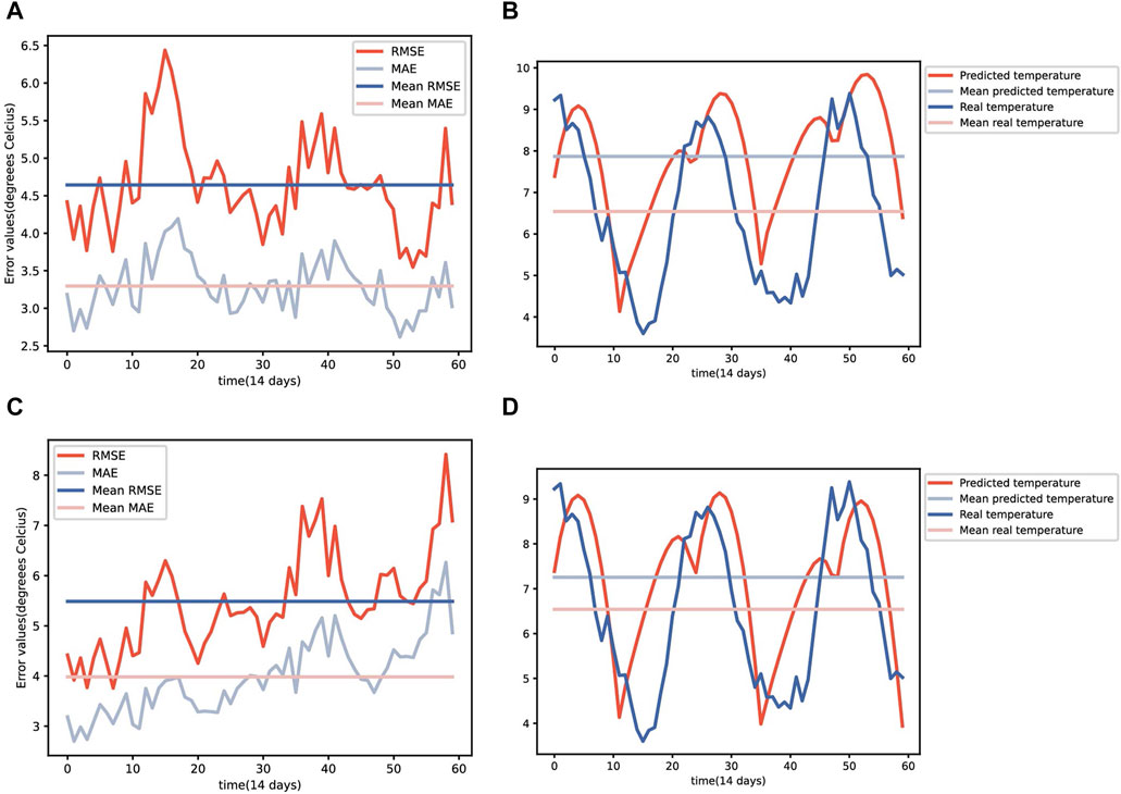
FIGURE 1. RMSE, MAE, and mean temperature change over the Earth. The RMSE and MAE in each time step based solely on real images (A) the mean temperature change over the Earth that the model predicted solely on real images (B). RMSE and MAE in each time step by feeding generated images (C) the mean temperature change over the Earth the model predicted by feeding generated images (D).

Figure 2A shows the model prediction of the temperature on 15 December 2022, and the temperature observed on that date. The predicted image was much more blurred than the observed image. While the right image shows much more precise delineations of the color change, the left image has more or less equal colors for regions where the color should be different. However, differences are present that clearly divide the continental and oceanic regions in the left image, even though the temperature difference is not well described in the image. Moreover, the temperatures of the regions closer to the equator are predicted to be hotter (more yellow), whereas the regions near the poles are predicted to be colder (more blue).

FIGURE 2

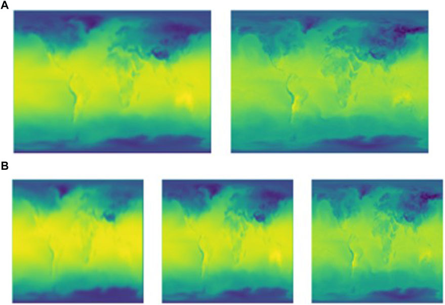
FIGURE 2. Predicted temperature on 15 December 2022. (A) Left image is the image generated by the model, and right image is the image derived from real data solely from real images. (B) Left image generated by the model when fed autoregressively; middle image generated by the model when trained on all real images when fed autoregressively; right image derived from data when fed autoregressively.

Figure 3A displays the RMSE/MAE values over every predicted time step in each major region of Earth. The model was the best at predicting the temperature in the South African region, with the lowest RMSE and MAE of 2.222 and 1.822, respectively. The model was the least effective at predicting the temperature in Northwest Asia, exhibiting high RMSE and MAE values of 6.829 and 5.657, respectively. Figure 3B shows the change in the mean temperature of each region of the predicted versus the actual data. The Arctic and Antarctic regions can be easily predicted using the model, whereas regions such as Oceania/Southeast Asia, South America, North Africa, and South Africa cannot be predicted well using the model. The remaining regions—Northwest Asia, South Asia, East Asia, North America, and Europe—appear to have relatively good accuracy, exhibiting minimal deviation between the predicted mean temperature and the real mean temperature and little change between the increase and decrease patterns.

FIGURE 3

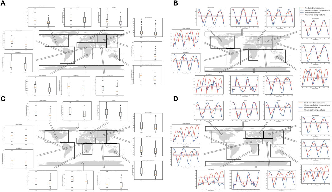
FIGURE 3. RMSE, MAE (A) and change in mean temperature (B) over each region trained solely on real images. RMSE, MAE (C), and change in mean temperature (D) over each region trained solely by feeding in generated images.

3.2 Analysis of the output generated by feeding generated images

The model still exhibited reasonable performance with this approach, with RMSE and MAE values of 5.487 and 3.982, respectively. However, both MAE and RMSE values increased when compared with the results in Section 3.1: RMSE and MAE of 4.642 and 3.296, respectively. Figure 1 shows the RMSE and MAE values over each time step as a line graph (c) and the average temperature change of the Earth over time for both the predicted and real values (d). The temperature pattern slightly increases over time, greater than the actual data. In addition, the predicted temperature was higher than the predictions based solely on the real images.

Figure 2B shows the model predictions of the temperature on 15 December 2022, and the temperature observed on that date. The left image shows the image generated when the output was generated on the generated images; the middle image shows the image generated when the output was generated based on real images; and the right image shows the image of real data. While the images look similar, the region around the equator on the left image is the most yellow, indicating the warmest of the three images. The middle image has an Arctic and Antarctic region that is the bluest, indicating the coldest of the three images. The leftmost image is the blurriest, yet the major delineations (i.e., continents) are still somewhat recognizable.

Figure 3C depicts all RMSE/MAE values over every predicted time step and the change in the mean temperature of each region of the predicted versus the actual data in each major region of Earth. South Africa remained the region where the model predicted the best, with the lowest RMSE and MAE values of 2.998 and 2.510, respectively. The least effective region predicted by the model remained Northwest Asia, with the highest RMSE values of 8.304 and 6.957. Figure 3D shows that the model is ineffective in predicting the mean temperatures in Europe, South Asia, Oceania, Southeast Asia, South America, North Africa, and South Africa.

3.3 Temperature model prediction

The model’s output of the mean temperature over the next 20 years is shown in Supplementary Figure S2. The prediction accuracy of the model progressively deteriorates as time progresses. Predictions get blurrier and blurrier, and while the Arctic region first turns yellow, the Antarctic region does not follow this trend and remains cold. Figure 4 shows the mean temperature of each time step over the next 20 years. The time was shown per month in order to make the chart clearer. The model projects that the temperature will reach an average of roughly 18°C in the next 20 years, roughly an increase of 11°C. However, seasonal patterns of increase and decrease in temperature can still be observed in the predictions, although the degree of increase and decrease varies over time and the small pattern of slight decrease near July enlarges.

FIGURE 4

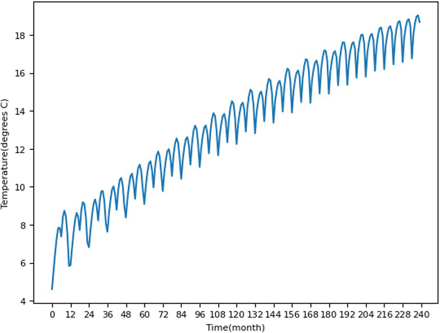
FIGURE 4. Temperature progression versus time into the future. The time spans from 1/1/2022 to 31/12/2041.

4 Discussion

Based on an autoregressive LSTM network, we developed a climate predictive model, particularly long-term temperature, with reasonable performance. Although future climate predictions are vital for addressing the challenges posed by global warming, only a few models have been developed to detect long-term climate change. Future climate predictions can be crucial in decision-making, policy planning, prevention and response to natural disasters, resource management, and environmental protection.

The LSTM model, a type of recurrent neural network, is adept at capturing long-term dependencies in time series data, making it effective for modeling and predicting complex climate patterns (Gers and Schmidhuber, 2000). With a memory cell capable of storing and retrieving information over extended periods, LSTMs can crucially remember features and patterns from earlier time steps, enhancing the understanding of climate variable dynamics. Their ability to handle diverse input types simultaneously is vital for climate prediction, where various meteorological variables contribute to the overall system (Wu et al., 2024). LSTMs are robust against noise and uncertainties in climate data, contributing to improved prediction accuracy. They excel when trained on large and complex climate datasets, learning intricate patterns and dependencies. The adaptive learning capability allows LSTMs to adjust internal parameters based on input data characteristics, capturing the non-linear and dynamic nature of climate processes (Ewees et al., 2022). Configurable for predicting values at multiple future time steps, LSTMs are suitable for both short-term and long-term climate predictions, crucial for understanding trends and variations over different time scales in climate modeling.

GCMs, as complex computer-based models, incorporate various components of the Earth’s system, providing insights into a wide range of climate variables such as temperature, precipitation, wind patterns, atmospheric circulation, and risk of climate change. Owing to their limitations and uncertainties, exploring more detailed relationships between emissions and multiregional climate responses requires applying GCMs that allow climate behavior to be simulated under various conditions on decadal to multi-centennial timescales (Bitz and Polvani, 2012; Nowack et al., 2017; Hartmann et al., 2019). However, modeling climate at increasingly high spatial resolutions has significantly increased computational complexity. Numerous studies have been conducted to develop AI models to address this issue and supplement these models.

A study predicting global long-term climate change patterns from short-term simulations evaluated the performance using Ridge and Gaussian Process Regression (GPR) at the grid-cell level. Both approaches predicted broad features such as enhanced warming over the Northern Hemisphere, like pattern scaling (Mansfield et al., 2020). The temperature error in this study remains between one and two degrees, which was significantly lower than that in the present study. Mansfield et al. also conducted analysis of their results based on the different regions. The region showing effective prediction and less effective prediction is somewhat different. than that of our study. In some regions (e.g., East Asia) the dominant coefficients appear in regions close to the predicted grid cell, whereas in other regions (e.g., Europe) predictions are strongly influenced by the short-term responses over relatively remote areas, such as sea-ice regions over the Arctic. Our study and Mansfield et al.’s study both predicts the East Asia region well, which adds value to this study’s model. However, their study mainly focused on improving the GCMs, whereas this study aims to replace the GCMs. As a corollary, their study was pulled from the outputs of GCMs, whereas this study’s outputs were from reanalysis data. In addition, the errors in that study were calculated at the grid-cell level, which can be misleading because they penalize patterns in which broad features are predicted correctly but are displaced marginally on the spatial grid (Rougier, 2016). This crucial predicted difference in the data could be the leading cause of the difference in errors between the present study and those reported by Mansfield et al. The use of different ML algorithms (Autoregressive LSTM versus Gaussian/Ridge regression) could also have contributed to this difference.

A study on global mean surface temperature projections employing advanced ensemble methods and past information has been reported (Stobach and Bel, 2020). This study did not implement the RMSE as a metric. The study predicted the change in global mean temperature, projected to be a maximum of 4°C increase, even though it depends on the type of algorithm implemented. This value represents a large difference from the projected increase in temperature in this study, which could be due to the difference in ML algorithms (Autoregressive LSTM vs. ensemble models) and differences in data. The differences can also be explained based on the same reasons as those regarding Mansfield et al. reported in the previous paragraph.

Large-scale spatial patterns of precipitation across the western United States were forecasted by training on thousands of seasons of climate model simulations and testing on the historical observational period (1980–2020). The results were similar to or outperformed existing dynamical models from the North American Multi-Model Ensemble (Gibson et al., 2021). The study implemented numerous ML models, such as LSTM, NN, XGBoost, and Random Forest algorithm, to predict the precipitation of North America. Their LSTM model was a consistent performer, with an accuracy score of roughly 0.5 for all categories. This prediction is higher than in the other models tested in the study. Our model has relatively reasonable errors, similar to this previous study. Nevertheless, we explored the feasibility of training various ML approaches on a large climate model ensemble, providing a long training set with physically consistent model realizations.

Previous researchers have also utilized Convolutional Neural Networks for weather prediction (Scher and Messori, 2019; Weyn et al., 2019). The error in Weyn’s study increased rapidly, increasing every 12 h, compared to the longer rate in ours. This is mainly because the data in the study were taken every 6 h. In contrast, in this study, we obtained data effectively every 2 weeks. Nevertheless, our prediction length with a relatively low RMSE (sixty-time steps) is much longer than that reported by Weyn et al. It is important to note, however, that Weyn et al.’s study attempted to predict the 500-hPa geopotential height, which could change the entirety of the study’s result. Moreover, the modeling approach used by Scher and Messori was limited in that a poor seasonal cycle and unrealistic predictions were considered when trained for long periods. In this study, although still producing unrealistic predictions, seasonal cycles were successfully predicted for up to 20 years, improving the results reported by Scher and Messori. Similarly, Scher and Messori predicted the 500-hPa geopotential height, which makes a direct comparison of the error values meaningless. The reason is the different model architectures utilized (i.e., autoregressive LSTM, Convolutional Neural Network) because the data used are both ERA5 reanalysis.

This study showed that an autoregressive LSTM architecture improved the long-term climate predictions of ML models. However, there are several limitations. The proposed model can be seen as underfitting. Although the model succeeds in learning the general patterns in the climate, the model cannot learn the smaller patterns within the continents effectively. The flattening of oceans and land can be shown. The predictions turn out to be somewhat unrealistic when repeated for long durations of time. However, these limitations might be overcome by increasing the complexity of the model, such as by using denser layers, more filters, and increasing the amount of training data. More realistic predictions can be made in the future if more complex models and sufficient computational processing to accommodate them are reflected. In addition, the reasoning behind why the model made these predictions cannot be easily distinguished. Utilizing Explainable AI tools to understand the reasoning behind such predictions would also be helpful.

This study’s model served solely as the baseline model. With several improvements, the model could reach its full potential. The ability of this architecture to make it successful compared with other architectures (i.e., the possibility of predicting global patterns over a long period) was demonstrated in this study, providing a novel insight of a novel AI model that can be utilized for climate prediction purposes.

In conclusion, the potential of using autoregressive LSTM models for climate prediction was considered in this study. The model outputted reasonable predictions of the global temperature at 2 m for a long period of time. The model successfully predicted the global mean temperature progression of multiple regions. This feature has not been achieved in previous studies based on Neural Networks, making this study practical. The model developed in this study should be used as a baseline for further development with increased computing power and data availability.

Data availability statement

Publicly available datasets were analyzed in this study. This data can be found here: ERA5 reanalysis ensemble mean data. Refer to this link: https://cds.climate.copernicus.eu/cdsapp#!/dataset /reanalysis-era5-single-levels?tab=overview.

Author contributions

SC: Conceptualization, Data curation, Formal Analysis, Methodology, Visualization, Writing–original draft, Writing–review and editing. VL: Conceptualization, Supervision, Writing–review and editing, Methodology.

Funding

The author(s) declare that no financial support was received for the research, authorship, and/or publication of this article.

Acknowledgments

We would like to acknowledge the Inspirit X AI mentorship program for facilitating this study.

Conflict of interest

The authors declare that the research was conducted in the absence of any commercial or financial relationships that could be construed as a potential conflict of interest.

Publisher’s note

All claims expressed in this article are solely those of the authors and do not necessarily represent those of their affiliated organizations, or those of the publisher, the editors and the reviewers. Any product that may be evaluated in this article, or claim that may be made by its manufacturer, is not guaranteed or endorsed by the publisher.

Supplementary material

The Supplementary Material for this article can be found online at: https://www.frontiersin.org/articles/10.3389/fenvs.2024.1301343/full#supplementary-material

SUPPLEMENTARY FIGURE S1 | Architecture of auto-regressive neural network models. The first 24 inputs are utilized as “warmup,” and the output of the final input is continuously fed through the model to generate the predictions.

SUPPLEMENTARY FIGURE S2 | A video showing temperature progression into the future. The time spans from 31/12/2022 to 31/12/2041.

References

Abadi, M., Agarwal, A., Barham, P., Brevdo, E., Chen, Z., Citro, C., et al. (2016). Tensorflow: large-scale machine learning on heterogeneous distributed systems. https://arxiv.org/abs/1603.04467.

Google Scholar

Bitz, C. M., and Polvani, L. M. (2012). Antarctic climate response to stratospheric ozone depletion in a fine resolution ocean climate model. Geophys. Res. Lett. 39 (20), L20705. doi:10.1029/2012GL053393

CrossRef Full Text | Google Scholar

Chai, T., and Draxler, R. R. (2014). Root mean square error (RMSE) or mean absolute error (MAE)? – Arguments against avoiding RMSE in the literature. Geosci. Model Dev. 7 (3), 1247–1250. doi:10.5194/gmd-7-1247-2014

CrossRef Full Text | Google Scholar

Chollet, F. (2015). Keras: deep learning library for theano and tensorflow. Accessed https://keras.io/.

Google Scholar

Collins, M. J., Chandler, R. B., Cox, P. T., Huthnance, J. M., Rougier, J., and Stephenson, D. B. (2012). Quantifying future climate change. Nat. Clim. Change 2 (6), 403–409. doi:10.1038/nclimate1414

CrossRef Full Text | Google Scholar

Düben, P., and Bauer, P. (2018). Challenges and design choices for global weather and climate models based on machine learning. Geosci. Model Dev. 11 (10), 3999–4009. doi:10.5194/gmd-11-3999-2018

CrossRef Full Text | Google Scholar

Edwards, P. N. (2010). History of climate modeling. Wiley Interdiscip. Rev. Clim. Change 2 (1), 128–139. doi:10.1002/wcc.95

CrossRef Full Text | Google Scholar

Ewees, A. A., Al-qaness, M. A., Abualigah, L., and Elaziz, M. A. (2022). HBO-LSTM: optimized long short term memory with heap-based optimizer for wind power forecasting. Energy Convers. Manag. 268, 116022. doi:10.1016/j.enconman.2022.116022

CrossRef Full Text | Google Scholar

Gale (2022). UN report: climate Change is irrevocalble. Accessed https://link.gale.com/apps/doc/A693733918/SCIC?u=wall96493&sid=bookmark-SCIC&xid=f30c64a2.

Google Scholar

Gers, F. A., and Schmidhuber, J. (2000). “Proc. IEEE-INNS-ENNS international joint conference on neural networks. IJCNN 2000. Neural computing: new challenges and perspectives for the new millennium,” in Proceedings of the IEEE-INNS-ENNS International Joint Conference on Neural Networks. IJCNN 2000. Neural Computing: New Challenges and Perspectives for the New Millennium, Como, Italy, July, 2000.

Google Scholar

Gibson, P. B., Chapman, W. E., Altinok, A., Monache, L. D., DeFlorio, M. J., and Waliser, D. E. (2021). Training machine learning models on climate model output yields skillful interpretable seasonal precipitation forecasts. Commun. Earth Environ. 2, 159. doi:10.1038/s43247-021-00225-4

CrossRef Full Text | Google Scholar

Hartmann, D. L., Blossey, P. N., and Dygert, B. D. (2019). Convection and climate: what have we learned from simple models and simplified settings? Curr. Clim. Change Rep. 5, 196–206. doi:10.1007/s40641-019-00136-9

CrossRef Full Text | Google Scholar

Herman, G. S., and Schumacher, R. S. (2018). Money doesn’t grow on trees, but forecasts do: forecasting extreme precipitation with random forests. Mon. Weather Rev. 146 (5), 1571–1600. doi:10.1175/mwr-d-17-0250.1

CrossRef Full Text | Google Scholar

Hersbach, H., Bell, B., Berrisford, P., Biavati, G., Horányi, A., Muñoz Sabater, J., et al. (2023). ERA5 hourly data on single levels from 1940 to present. Copernic. Clim. Change Serv. (C3S) Clim. Data Store (CDS). doi:10.24381/cds.adbb2d47

CrossRef Full Text | Google Scholar

Hewamalage, H., Bergmeir, C., and Bandara, K. (2021). Recurrent neural networks for time series forecasting: current status and future directions. Int. J. Forecast. 37 (1), 388–427. doi:10.1016/j.ijforecast.2020.06.008

CrossRef Full Text | Google Scholar

Hurrell, J. W. (2003). “Climate variability. North atlantic and arctic oscillation,” in Encyclopedia of atmospheric sciences.

Google Scholar

Kaur, J., Parmar, K. S., and Singh, S. (2023). Autoregressive models in environmental forecasting time series: a theoretical and application review. Environ. Sci. Pollut. Res. 30 (8), 19617–19641. doi:10.1007/s11356-023-25148-9

CrossRef Full Text | Google Scholar

Kulkarni, G., Muley, A., Deshmukh, N., and Bhalchandra, P. (2018). Autoregressive integrated moving average time series model for forecasting air pollution in Nanded city, Maharashtra, India. Model. Earth Syst. Environ. 4 (4), 1435–1444. doi:10.1007/s40808-018-0493-2

CrossRef Full Text | Google Scholar

Kumar, A., and Hoerling, M. P. (1995). Prospects and limitations of seasonal atmospheric GCM predictions. Bull. Am. Meteorological Soc. 76 (3), 335–345. doi:10.1175/1520-0477(1995)076<0335:palosa>2.0.co;2

CrossRef Full Text | Google Scholar

Lerner, K. L. (2023). “Climate change,” in Gale science online collection (Farmington Hills, Michigan, United States: Gale). Accessed https://link.gale.com/apps/doc/KODPIQ908201214/SCIC?u=wall96493&sid=bookmark-SCIC&xid=97316fbe.

Google Scholar

Mansfield, L., Nowack, P., Kasoar, M., Everitt, R. G., Collins, W. J., and Voulgarakis, A. (2020). Predicting global patterns of long-term climate change from short-term simulations using machine learning. Npj Clim. Atmos. Sci. 3 (1), 44. doi:10.1038/s41612-020-00148-5

CrossRef Full Text | Google Scholar

Nowack, P. J., Braesicke, P., Luke Abraham, N., and Pyle, J. A. (2017). On the role of ozone feedback in the ENSO amplitude response under global warming. Geophys. Res. Lett. 44 (8), 3858–3866. doi:10.1002/2016GL072418

PubMed Abstract | CrossRef Full Text | Google Scholar

Pachauri, R. K., Allen, M. R., Barros, V. R., Broom, J., Cramer, W., Christ, R., et al. (2015). Climate change 2014: synthesis report. Accessed https://www.ipcc.ch/site/assets/uploads/2018/02/SYR_AR5_FINAL_full.pdf.

Google Scholar

Razak, N. A., Aris, A. Z., Ramli, M., Looi, L. J., and Juahir, H. (2016). Temporal flood incidence forecasting for Segamat River (Malaysia) using autoregressive integrated moving average modelling. J. Flood Risk Manag. 11, S794–S804. doi:10.1111/jfr3.12258

CrossRef Full Text | Google Scholar

Rougier, J. (2016). Ensemble averaging and mean squared error. J. Clim. 29, 8865–8870. doi:10.1175/jcli-d-16-0012.1

CrossRef Full Text | Google Scholar

Scher, S. (2018). Toward data-driven weather and climate forecasting: approximating a simple general circulation model with deep learning. Geophys. Res. Lett. 45. doi:10.1029/2018GL080704

CrossRef Full Text | Google Scholar

Scher, S., and Messori, G. (2019). Weather and climate forecasting with neural networks: using general circulation models (GCMs) with different complexity as a study ground. Geosci. Model Dev. 12 (7), 2797–2809. doi:10.5194/gmd-12-2797-2019

CrossRef Full Text | Google Scholar

Schneider, P., and Xhafa, F. (2022). Chapter 3–anomaly detection: concepts and methods. Amsterdam, Netherlands: Elsevier eBooks, 49–66. doi:10.1016/b978-0-12-823818-9.00013-4

CrossRef Full Text | Google Scholar

Shi, X., Chen, Z., Wang, H., Yeung, D. Y., Wong, W. K., and Woo, W. C. (2015). "Convolutional LSTM Network: a machine learning approach for precipitation nowcasting,” in Proceedings of the 28th International Conference on Neural Information Processing Systems-Volume 1(NIPS 2015). Editor C. Cortes, N. Lawrence, D. Lee, M. Sugiyama, and R. Garnett (Cambrdige, MA: MIT Press).

Google Scholar

Stern, P. C., and Easterling, W. E. (1999). Making climate forecasts matter. Washington, D.C., United States: National Academies Press eBooks. doi:10.17226/6370

CrossRef Full Text | Google Scholar

Strobach, E., and Bel, G. (2020). Learning algorithms allow for improved reliability and accuracy of global mean surface temperature projections. Natl. Commun. 11, 451. doi:10.1038/s41467-020-14342-9

PubMed Abstract | CrossRef Full Text | Google Scholar

Weyn, J. A., Durran, D. R., and Caruana, R. (2019). Can machines learn to predict weather? Using deep learning to predict gridded 500-hPa geopotential height from historical weather data. J. Adv. Model. Earth Syst. 11 (8), 2680–2693. doi:10.1029/2019ms001705

CrossRef Full Text | Google Scholar

Wu, Y., Meng, X., Zhang, J., He, Y., Romo, J. A., Dong, Y., et al. (2024). Effective LSTMs with seasonal-trend decomposition and adaptive learning and niching-based backtracking search algorithm for time series forecasting. Expert Syst. Appl. 236, 121202. doi:10.1016/j.eswa.2023.121202

CrossRef Full Text | Google Scholar