Analysis of Molecular Variance (AMOVA) for Autopolyploids

Introduction

Autopolyploidy is an important, but often overlooked, aspect of the evolution of all major groups of Eukaryotes-plants, animals, and fungi- and may constitute an underappreciated source of biodiversity (Hardy, 2015). There are many species in which multiple ploidy levels (cytotypes) exist and often each cytotype itself conforms to the requirements of several widely used species concepts (Soltis et al., 2007). Autopolyploidy has many effects on the mechanisms of evolution, not only because of the increase in genomic content and the flexibility for developing new traits (Larkin et al., 2016), but also because, compared to diploidy, it generates different dynamics of allele frequencies that interact with various demographic processes, influencing adaptation and speciation (Parisod et al., 2010). In a species with different ploidy levels, the different cytotypes often show intricate geographical patterns in their distribution, which may be the result of historical, demographic, ecological, or genetic processes (Glennon et al., 2014; Kolár et al., 2017). The analysis of population genetic structure of autopolyploids may therefore reveal a lot about these processes. However, polyploids also present several challenges to the researchers studying their population genetics (Dufresne et al., 2014). This is because population genetic theory, the expectations derived from this theory, and the statistical tools for data analysis were developed mostly for haploids and diploids and require translation for polyploids (Meirmans et al., 2018).

Several of the basic genetic processes work differently in autopolyploids than in diploids (Meirmans et al., 2018). The higher number of chromosomes means that for each gene a higher total number of copies is present in a population. This increases the number of mutation events per population, and also increases the impact of migration as each migrant individual carries more chromosome copies to its new population. Conversely, the higher total number of chromosome copies is akin to a higher effective population size and therefore reduces the force of genetic drift, compared to a diploid population with the same number of individuals. Mendelian segregation also works differently in autopolyploids, since it is not necessarily completely random, as is almost always the case in diploids. Instead, there may be disomic inheritance, polysomic inheritance, or a combination of the two, where the rate of polysomy varies across the genome (Stift et al., 2008; Meirmans and van Tienderen, 2013). In addition, autopolyploids may show double reduction, a process where two copies of the same chromatid segment end up in the same gamete (Bever and Felber, 1992; Hardy, 2015). For example in a autotetraploid with genotype ABCD this may lead to the production of homozygous (AA, BB, CC, and DD) gametes, in addition to the expected heterozygous gametes (e.g., AB, AD). A more practical problem in the genetic analysis of polyploids is that it is often difficult to estimate the dosage of the different alleles in a genotype (Dufresne et al., 2014). For example, it may be impossible to distinguish between the triploid genotypes AAB and ABB since they both share the marker phenotype AB. Missing dosage information may introduce a bias in the subsequent analysis; though depending on the type of analysis this bias may be corrected for quite effectively when random mating in populations can be assumed (De Silva et al., 2005; Meirmans et al., 2018). However, when the assumption of Hardy Weinberg equilibrium cannot be made for a species, accounting for the missing dosage information becomes more problematic, though in some cases it is possible to adjust the calculations specifically to take the missing dosage into account (Hardy, 2015; Field et al., 2017).

Estimating the strength of the genetic population structure is usually done using F-statistics that decompose the genetic variance into within-individual, within-population and among-population components (Wright, 1969). Autopolyploidy affects the way these statistics should be estimated (Meirmans et al., 2018), but also their expected values under a given model of population structure, when compared to the same model for diploids (Ronfort et al., 1998). For example, the expected value of F_ST—quantifying the degree of population differentiation—depends on the balance among migration, mutation, and drift. In autopolyploids, the increased effects of mutation and migration, in combination with the reduced force of drift, cause the expected value of F_ST to be lower than the corresponding value for diploids (Meirmans et al., 2018). This difference in expectation complicates comparisons of the strength of population structure among species or sets of populations with different ploidy levels.

To enable a better estimation of the degree of population differentiation across ploidy levels, Ronfort et al. (1998) developed an alternative summary statistic, which they called ρ, for which the expected value is independent of the ploidy level. The ρ-statistic is comparable to F_ST in that it estimates the degree of population differentiation and—barring estimation error—ranges between 0 and 1. For haploid data, the value of ρ is exactly the same as the value of F_ST; for higher ploidy levels, the value of ρ is generally slightly higher than that of F_ST. The ploidy independence of ρ is achieved by disregarding the within-individual variation (illustrated by Equation 14 below). Another perk of the ρ-statistic that makes it suitable for the analysis of polyploid data is that its value is both independent of the rate of double reduction (Ronfort et al., 1998) and of the frequency of polysomic inheritance (Meirmans and van Tienderen, 2013). The ρ-statistic also has a major advantage that is applicable to diploid as well as polyploid data: its value is independent of the rate of self-fertilization or other forms of inbreeding. This means that under a given model of population structure, ρ will have the same value for a strict inbreeder as for an obligate outcrosser, whereas F_ST gives higher values for inbreeders than for outcrossers. This is especially useful in comparative studies, where a comparison of F_ST and ρ can be used to see whether differences in population structure are due to differences in mating system or due to differences in population connectivity. Unfortunately, ρ is not very widely used, possibly because there are only few computer programs that allow estimation of ρ from genetic marker data. The only two such programs that we are aware of are SPAGEDI (Hardy and Vekemans, 2002), and GENODIVE (Meirmans and van Tienderen, 2004).

One of the most popular methods for estimating F-statistics is via Analysis of Molecular Variance (AMOVA) (Excoffier et al., 1992; Peakall et al., 1995; Michalakis and Excoffier, 1996). This popularity is probably due to the remarkable flexibility of the AMOVA framework: it can be used for the estimation of different types of F-statistics (F_ST, φ_ST, R_ST) and can easily incorporate additional hierarchical levels of population structure (e.g., testing for differentiation among groups of populations). In addition, AMOVA can be used to detect population clustering in a genetic dataset (Dupanloup et al., 2002; Meirmans, 2012). However, AMOVA has been described only for haploid and diploid data and the link between the AMOVA framework and the ρ-statistic has not been explored theoretically.

In this paper, we outline how the AMOVA framework can be extended to include autopolyploid data. We start by discussing how the standard AMOVA, for calculating F_ST, φ_ST, or R_ST, can be easily adapted for use with autopolyploids. We then show how the ploidy-independent ρ-statistic can be calculated in AMOVA by using a matrix of squared Euclidean distances between individuals, calculated from the within-individual allele frequencies. Finally, we show the application of the method by calculating both F_ST and ρ for simulated datasets and discuss how to deal with the polyploidy-specific complication of missing dosage information.

The AMOVA Framework

General Approach

In AMOVA (Excoffier et al., 1992; Michalakis and Excoffier, 1996), F-statistics are calculated from a set of covariance components, corresponding to the different hierarchical levels assumed to be present in the population structure (following Cockerham, 1973; Weir and Cockerham, 1984). So under a simple model of population structure where individuals are distributed over a number of populations, we can decompose the total genetic variance (${\sigma }_T^2$) into among-populations (${\sigma }_a^2$), among-individuals within populations (${\sigma }_b^2$), and within-individuals (${\sigma }_c^2$) covariance components, such that ${\sigma }_T^2$ = ${\sigma }_a^2$+${\sigma }_b^2$+${\sigma }_c^2$. The F-statistics can then be calculated as simple ratios of those covariance components:

$\begin{array}{rcll}{F}_{ST}& =& \frac{{\sigma }_a^2}{{\sigma }_T^2}& (1\text{a})\end{array}$

$\begin{array}{rcll}{F}_{IS}& =& \frac{{\sigma }_b^2}{{\sigma }_b^2+{\sigma }_c^2}& (1\text{b})\end{array}$

$\begin{array}{rcll}{F}_{IT}& =& \frac{{\sigma }_a^2+{\sigma }_b^2}{{\sigma }_T^2}& (1\text{c})\end{array}$

When the populations can be clustered into multiple groups, an extra hierarchical level is added and the total genetic variance is decomposed into among-groups (${\sigma }_a^2$), among-populations within-groups (${\sigma }_b^2$), among-individuals within-populations (${\sigma }_c^2$), and within individuals (${\sigma }_d^2$) covariance components, such that ${\sigma }_T^2$ = ${\sigma }_a^2$+${\sigma }_b^2$+${\sigma }_c^2$+${\sigma }_d^2$. The corresponding F-statistics are then:

$\begin{array}{rcll}{F}_{CT}& =& \frac{{\sigma }_a^2}{{\sigma }_T^2}& (2\text{a})\end{array}$

$\begin{array}{rcll}{F}_{SC}& =& \frac{{\sigma }_b^2}{{\sigma }_b^2+{\sigma }_c^2+{\sigma }_d^2}& (2\text{b})\end{array}$

$\begin{array}{rcll}{F}_{IS}& =& \frac{{\sigma }_c^2}{{\sigma }_c^2+{\sigma }_d^2}& (2\text{c})\end{array}$

$\begin{array}{rcll}{F}_{IT}& =& \frac{{\sigma }_a^2+{\sigma }_b^2+{\sigma }_c^2}{{\sigma }_T^2}& (2\text{d})\end{array}$

This follows the Analysis of Variance framework that was developed earlier by Cockerham (1973) and Weir and Cockerham (1984). However, whereas Weir and Cockerham calculated these covariance components from a linear vector of allele frequencies, AMOVA calculates them using a matrix D of pairwise squared Euclidean distances. This is based on previous work by Li (1976) showing that conventional Sums of Squares can be calculated from a matrix of pairwise squared Euclidean distances. These Sums of Squares can then be used to calculate the Expected Mean Squares, which in turn can be used to calculate the covariance components (Weir and Cockerham, 1984).

The use of a distance metric is actually what gives AMOVA its remarkable flexibility, as the distance metric can be changed, depending on the type of data under analysis. A simple matching distance can be used for a single locus with allelic data—for example for SNPs (Peakall et al., 1995; Michalakis and Excoffier, 1996). Multilocus values of the F-statistics can then be obtained by summing the covariance components over loci. A distance metric for haplotypic data was described in the original paper by Excoffier et al. (1992), based on the phenetic distance between the pair of haplotypes. This is also the most frequently used method for sequence data, though more complex distance metrics can be used as well—e.g., by incorporating a specific mutational model or by tracing distances along a connecting network or tree (Excoffier and Smouse, 1994). A distance metric for microsatellites loci can be calculated by taking the squared difference in repeat number between alleles (Michalakis and Excoffier, 1996).

The interpretation of the F-statistics returned by AMOVA depends strongly on the choice of distance metric used. This means that from the wide array of available estimators for F_ST, different estimators are obtained by different distance metrics. For allelic data, where the simple matching distance is used, the resulting F-statistics are mathematically equivalent to the estimators of Weir and Cockerham (1984). In contrast, for haplotypic/sequence data, the distances are indicative of the evolutionary relationships between haplotypes/sequences (Whitlock, 2011); to reflect this, the F-statistics are generally referred to with the Greek letter φ. Finally, when for microsatellites the difference in repeat number is used, the estimator corresponds to the R_ST-statistic (Slatkin, 1995).

Adaptation to Autopolyploids

For autopolyploids, AMOVA can be performed using the same methods as above for calculating the pairwise distances among alleles, yielding estimates of F_ST, φ_ST, or R_ST. However, the higher ploidy means that the overall size of the complete distance matrix increases. So what is needed to adapt a standard diploid AMOVA to autopolyploid data is to account for this larger overall sample size in all the calculations, which is very straightforward when the data contain only a single ploidy level. For a total sample size of N diploids, the distance matrix is of size 2N*2N, whereas for autopolyploids with ploidy level x, the matrix is of size xN*xN (for computational efficiency it is also possible to only use the lower or upper half of the matrix). The Sums of Squares are therefore calculated by summing over a larger number of pairwise distances, though this follows the same approach as outlined by Excoffier et al. (1992; Their equations 8a−8c) by summing over groups, populations, and individuals as necessary.

The higher ploidy level results in a larger number of allele copies within individuals, populations, and groups. This larger number of allele copies needs to be reflected in the degrees of freedom used for calculating the Expected Mean Squares; however, this is only the case for the within-individual and total degrees of freedom, as the others are only determined by the higher-level sample sizes. In Table 1 we give generic formulas for the degrees of freedom for any ploidy x > 1 for a model with a single group of populations, and compare this to the diploid case described in the original papers (Excoffier et al., 1992; Peakall et al., 1995; Michalakis and Excoffier, 1996); the notation follows the notation used in the documentation of the software Arlequin (Excoffier and Lischer, 2010, 2015). Table 2 shows the same, but then for multiple groups of populations. The Expected Mean Squares can then be obtained by dividing the corresponding Sum of Squares by the degrees of freedom.

TABLE 1

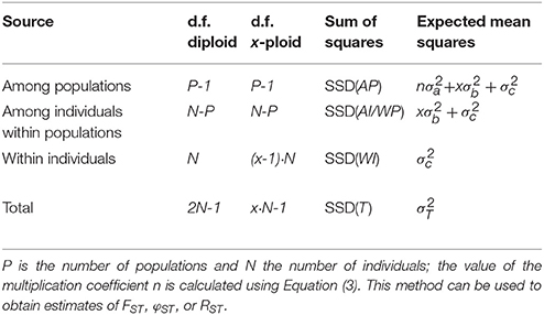
Table 1. Outline of the AMOVA framework for a single group of populations with the degrees of freedom (d.f.) both given for diploids and generalized for any ploidy level x (except haploid).

TABLE 2

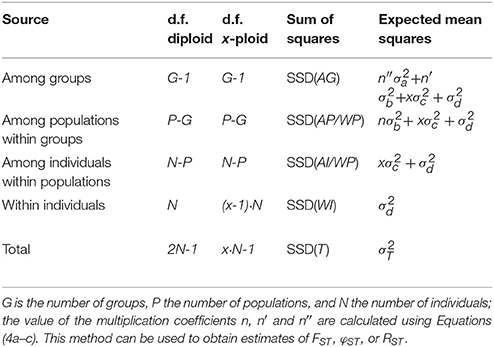
Table 2. Outline of the AMOVA framework for multiple group of populations with the degrees of freedom (d.f.) both given for diploids and generalized for any ploidy level x (except haploid).

For calculating the covariance components from the expected mean squares it is necessary to incorporate the sample sizes at the different hierarchical levels included in the analysis. The simplest case is a single group of populations all of the same ploidy level x and all with the same sample size N_p. In this case (Table 1), the multiplication factor n is defined as xN_p, the number of allele copies sampled per population. However, when there is unbalanced sampling (Table 1), this multiplication factor has to take the sample sizes for all populations separately into account:

$\begin{array}{rc}n=\frac{xN-{\displaystyle {\sum }_{p\in P}}\frac{x{N}_p^2}{N}}{P-1}& (3)\end{array}$

Here, N_p is the number of individuals sampled in population p.

When there are multiple groups of populations (Table 2) there are three coefficients: n, n′, and n″. When sampling is balanced, so with the same number of individuals sampled for every population and the same number of populations sampled in each of the G groups, n and n′ are defined as xN_p. As above, this is simply the number of allele copies sampled per population. The value of n″ is then defined as xN_g, the number of allele copies sampled per group of populations. However when sample sizes within populations and/or groups are unbalanced (Table 2), the sample sizes have to be taken into account for the calculation, and the three coefficients are defined as:

$\begin{array}{rc}n=\frac{xN-{\displaystyle {\sum }_{g\in G}}{\displaystyle {\sum }_{p\in g}}\frac{x{N}_p^2}{N_g}}{P-G}& (4\text{a})\end{array}$

$\begin{array}{rc}{n}^{\prime }=\frac{{\displaystyle {\sum }_{g\in G}}\frac{(N-N_g)}{N_g}{\displaystyle {\sum }_{p\in g}}x{N}_p^2}{N(G-1)}& (4\text{b})\end{array}$

$\begin{array}{rc}{n}^{″}=\frac{xN-\frac{{\displaystyle {\sum }_{g\in G}}x{N}_g^2}{N}}{G-1}& (4\text{c})\end{array}$

where N_g is the number of individuals sampled in group g. For haploid and diploid data (x = 1 and x = 2), these equations are the same as for the standard AMOVA (Michalakis and Excoffier, 1996; Excoffier and Lischer, 2015).

Mixed Ploidy Datasets

Slightly more complicated evolutionary scenarios involve multiple ploidy levels, either occurring in separate populations, or co-occurring in populations. In such a case, there is no single ploidy level x that can be used to calculate the degrees of freedom and the multiplication coefficients. However, when the ploidy level of every genotyped individual is known (e.g., through flow cytometry), this problem can be solved by using the number of allele copies sampled per population (C), rather than the number of individuals (N). Table 3 shows the formulas for the degrees of freedom for any mixture of ploidy levels (though all should be at least diploids) for a model with a single group of populations. The corresponding coefficients n, n′, and n″ are defined as (again following the notation from Excoffier and Lischer, 2015):

$\begin{array}{rcll}{S}_P& =& {{\displaystyle \sum }}_{p\in P}{{\displaystyle \sum }}_{i\in p}\frac{C_i^2}{C_p}& (5\text{a})\end{array}$

$\begin{array}{rcll}n& =& \frac{C-S_P}{N-P}& (5\text{b})\end{array}$

$\begin{array}{rcll}{n}^{\prime }& =& \frac{S_P-{\displaystyle {\sum }_{i\in N}}\frac{C_i^2}{C}}{P-1}& (5\text{c})\end{array}$

$\begin{array}{rcll}{n}^{″}& =& \frac{C-{\displaystyle {\sum }_{p\in P}}\frac{C_p^2}{C}}{P-1}& (5\text{d})\end{array}$

The F-statistics can then be calculated in the normal way, using Equations (1a–c). Note that when the significance of the population differentiation is tested by permuting individuals over populations, the number of allele copies in the permuted populations may differ from the original values. Therefore, the coefficients n, n′, and n″ will have to be recalculated for every permutation.

TABLE 3

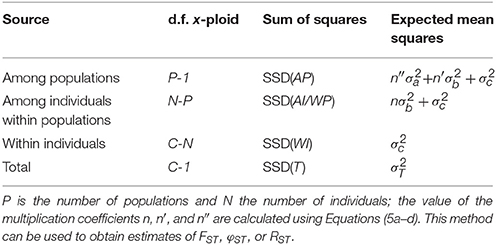
Table 3. Outline of the AMOVA framework for a single group of populations with the degrees of freedom (d.f.) for a mixture of individuals with different ploidy levels, based on the total number of allele copies sampled (C).

Ploidy-Independent ρ-Statistic

In addition to the above-developed method that yields estimates of F_ST, φ_ST, or R_ST, AMOVA can also be used to obtain estimates of the ploidy-independent ρ-statistic (Ronfort et al., 1998). Here we show that this can be done by performing AMOVA on a matrix of squared Euclidean distances calculated from the within-individual allele frequencies. Other than the above methods of calculating distances—where each distance is calculated between a pair of alleles or haplotypes—here each squared Euclidean distance (denoted as $d_{ij}^2$) is calculated between a pair of individual genotypes at a locus. The metric is calculated as

$\begin{array}{rc}{d}_{ij}^2={{\displaystyle \sum }}_{a=1}^A{(p_{ia}-p_{ja})}^2& (6)\end{array}$

where p_ia is the frequency of the ath allele (a ∈ {1, 2, …, A}) within individual i. In diploids, these frequencies can take the values 0, 0.5, and 1; in triploids the values 0, 0.33, 0.67, and 1; in tetraploids the values 0, 0.25, 0.5, 0.75, and 1; etc. For haploids, the only two possible values are 0 and 1 and therefore for haploids this metric is the same as the simple-matching distance; by extension this means that for haploid data the value of ρ equals that of F_ST.

This distance metric yields, for any ploidy level, only a single distance value per pair of individuals. As a result, the distance matrix is only of size N*N, whereas the approach above resulted in a matrix of xN*xN, for data of ploidy level x. The N*N matrix can then be used to perform AMOVA using the equations (not shown here) originally developed for haploid data in the paper by Excoffier et al. (1992). This approach also allows ρ to be calculated at different hierarchical levels, e.g., to compare differentiation among clusters of populations. For such use, we will adopt the convention of adding subscripts to indicate which levels are compared, though Ronfort et al. (1998) did not use any such subscripts in their original description of ρ. Note that since the within-individual component is disregarded, there are no ρ equivalents of F_IS and F_IT in such a hierarchical analysis.

When the two individuals have the same ploidy level, the squared Euclidean distance metric proposed here is a simple linear transformation of the squared Euclidean distance metric of Smouse and Peakall (1999). Since a linear transformation of the distance matrix does not affect the relative sizes of the variance components, this means that the Smouse and Peakall distance can also be used for AMOVA. However, the metric from Smouse and Peakall has only been defined for cases where the two individuals have the same ploidy level, whereas the metric proposed above is also suited to mixtures of different ploidy levels.

The mathematical relationship between the squared Euclidean distance metric and ρ can be deduced as follows. Again, p_ia refers to the frequency of the ath allele (a ∈ {1, 2, …, A}) in the ith individual (i ∈ {1, 2, …, N}). The sum of the D matrix can then be transformed as:

$\begin{array}{l}{\displaystyle {\sum }_{i=1}^N{\displaystyle {\sum }_{j=1}^N{d}_{ij}^2}}={\displaystyle {\sum }_{i=1}^N{\displaystyle {\sum }_{j=1}^N{\displaystyle {\sum }_{a=1}^A{\left(p_{ia}-p_{ja}\right)}^2}}}\\ =2N^2{\displaystyle {\sum }_{a=1}^A(\frac{1}{N}{\displaystyle {\sum }_{i=1}^N{p}_{ia}^2}}\\ -{\left(\frac{1}{N}{\displaystyle {\sum }_{i=1}^N{p}_{ia}}\right)}^2)& (7)\end{array}$

If we define

$\begin{array}{rc}{Ȟ}_O\equiv \frac{1}{N}{{\displaystyle \sum }}_{i=1}^N\left(1-{\sum }_{a=1}^A{p}_{ia}^2\right)& (8)\end{array}$

and

$\begin{array}{rc}{Ȟ}_E\equiv 1-{{\displaystyle \sum }}_{a=1}^A{\left(\frac{1}{N}{{\displaystyle \sum }}_{i=1}^N{p}_{ia}\right)}^2& (9)\end{array}$

then the sum of squared distances in Equation (7) can be simplified to:

$\begin{array}{rc}{{\displaystyle \sum }}_{i=1}^N{{\displaystyle \sum }}_{j=1}^N{d}_{ij}^2=2N^2({Ȟ}_E-{Ȟ}_O)& (10)\end{array}$

Ȟ_E and Ȟ_O as defined here are analogous—but not equivalent—to the standard H_E and H_O as defined by Nei (1987) for diploids and by Moody et al. (1993) for polyploids (see also Meirmans et al., 2018):

$\begin{array}{rc}{H}_O=\frac{1}{N}{{\displaystyle \sum }}_{i=1}^N\left(\left(1-{{\displaystyle \sum }}_{a=1}^A{p}_{ia}^2\right)·\frac{x_i}{x_i-1}\right)& (11)\end{array}$

$\begin{array}{rc}{H}_E=1-{{\displaystyle \sum }}_{a=1}^A{\left(\frac{{\displaystyle {{\displaystyle \sum }}_{i=1}^N}\left({x_i·p}_{ia}\right)}{{\displaystyle {{\displaystyle \sum }}_i^N}{x}_i}\right)}^2& (12)\end{array}$

While H_E and H_O attempt to correct the calculation of allele frequency or heterozygosity using individual ploidy information, Ȟ_E and Ȟ_O ignore such information, hence endowing ρ a ploidy-independent nature.

In the Island model where the number of populations is r (each population has a size of N), ρ_ST can be calculated as

$\begin{array}{rc}{\rho }_{ST}=1-\frac{{\left(r·N\right)}^2·x^2{{\displaystyle \sum }}_{k=1}^r{\displaystyle {\sum }_{i=1}^N}{\displaystyle {\sum }_{j=1}^N}{d}_{kij}^2}{r·N^2·x^2{\displaystyle {\sum }_{i=1}^{r·N}}{\displaystyle {\sum }_{j=1}^{r·N}}{d}_{ij}^2}& (13)\end{array}$

Using the link between the sum of squared distances and the Ȟ-statistics that was established in Equation (10), Equation (13) can be transformed into:

$\begin{array}{rc}{\rho }_{ST}=\frac{{Ȟ}_T-{Ȟ}_S}{{Ȟ}_T-{Ȟ}_O}& (14)\end{array}$

The statistic Ȟ_T is defined in the same vein as Ȟ_E but then for all populations together; Ȟ_S is the average of Ȟ_E calculated over populations. If the populations contain only a single ploidy level, Equation (14) can be transformed into

$\begin{array}{rc}{\rho }_{ST}=\frac{H_T-H_S}{H_T-H_O·\frac{x-1}{x}}& (15)\end{array}$

which is the same as Equation (6) in Meirmans et al. (2018).

Application to Data

Simulations Under a Hierarchical Island Model

To test how well the above-developed AMOVA framework performs for data with different ploidy levels, we simulated data under a standard hierarchical island model (Slatkin and Voelm, 1991; Vigouroux and Couvet, 2000). A set of 20 populations was simulated, divided into two archipelagoes, both having 10 populations. All populations had the same size of N = 100; mating within populations was completely random, including a probability of self-fertilization of 1/N. Genetic markers were simulated at 1,000 independently segregating loci; mutation followed a K-alleles model with 100 possible allelic states and a mutation rate of μ = 0.0001. Migration took place at different rates among populations from the same archipelago (m1) and among populations from different archipelagoes (m2).

The model was population-based, so individuals were not explicitly modeled but instead the populations were represented by a set of vectors containing the allele frequencies of all possible allelic states at all loci. Under the assumption of random mating, one generation of genetic drift can then easily be simulated by drawing random numbers from a multinomial distribution. For the expected values in the multinomial, we used the current population allele frequencies—after incorporating the expected effects of migration and mutation. For the number of draws in the multinomial, we used the number of chromosome copies in the population, so the population size multiplied by the ploidy level. The model was written in R, using the rmultinom() function for drawing random numbers; the used R-script is available in online Supplement 1 (Data Sheet 1).

The model was run for diploids, tetraploids, and hexaploids, for values of m2 of 0.001, 0.0001, and 0.00001; per value of m2 a range of values of m1 was used with a maximum of 0.1 and a minimum equal to the value of m2 (so m1 ≥ m2). Per scenario, the model was run once for 20,000 generations; replication was provided by the use of the 1,000 independent loci. After the last generation, genotypes were constructed by randomly distributing the alleles over individuals and written to a file. The software GENODIVE v. 2b27 (Meirmans and van Tienderen, 2004) was used to perform a hierarchical AMOVA on the resulting genotypes. The results were compared to the theoretical expectations for F_SC and F_CT derived by Vigouroux and Couvet (2000). Though these expectations were only derived for diploids, general results for any ploidy level x can be obtained by substituting all occurrences of the term “4N” in the equations by the term “2xN” (see Meirmans et al., 2018). The expectations for ρ for any ploidy level are equivalent to the expectation for F_ST under haploidy (Ronfort et al., 1998; Meirmans et al., 2018), so can also be derived from the equations of Vigouroux and Couvet (2000) by substituting every “4N” by “2N.”

Simulation Results

When applying the AMOVA framework to the simulated data for several ploidy levels, the results closely matched the theoretical expectations (Figure 1), indicating that AMOVA correctly estimates the variance components and the F-statistics. For all three values of m2, F_SC showed a monotonic decrease with increasing values of m1 (Figure 1, top row), whereas F_CT showed a monotonic increase (Figure 1, bottom row). As random mating within populations was assumed, the values of F_IS were close to zero for all simulated scenarios (not shown). The only slight deviation between the results of the simulation and the theoretical expectations was observed for the F_CT-statistic when the migration rate within archipelagoes (m1) was close to or equal to the migration rate between archipelagoes (m2). This deviation can easily be explained since the theoretical derivations of Vigouroux and Couvet (2000) assume that m1 > m2. For the cases where m1 = m2, the simulations consistently show a F_CT value that is close to zero, whereas the expected values are slightly higher.

FIGURE 1

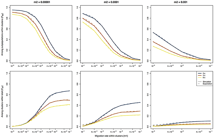
Figure 1. F-statistics calculated using an AMOVA on data of three different ploidy levels simulated using a hierarchical island model of migration. The solid lines represent the results of the simulations, the dashed lines represent the expected values based on the derivations of Vigouroux and Couvet (2000).

As expected, there is a strong difference between the F-statistics (Figure 1) and the ρ-statistics (Figure 2) in how they behave under different ploidy levels. For the F-statistics, at a given set of migration rates, the values decrease with increasing ploidy level. This is due to the increased impact of migration at higher ploidy levels combined with a decrease in the force of genetic drift (Meirmans et al., 2018). On the other hand, the ρ-statistics generally have similar values for all ploidy levels when calculating the differentiation among subpopulations within clusters (ρ_SC) or the differentiation among clusters (ρ_CT). This ploidy-independence of the ρ-statistic is immediately evident from the almost completely overlapping lines in Figure 2. As we saw above for F_CT, the estimates of ρ_CT from the simulated data show a slight deviation from the expected values when the assumption of m1 > m2 is violated.

FIGURE 2

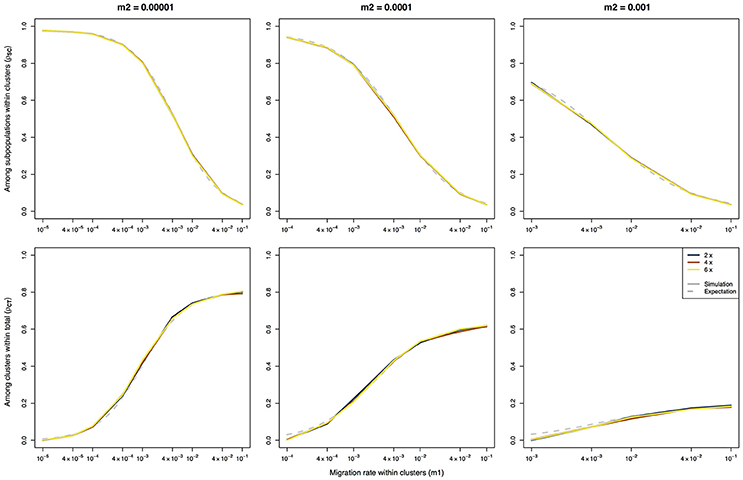
Figure 2. Ploidy-independent ρ-statistics calculated using an AMOVA on data of three different ploidy levels simulated using a hierarchical island model of migration. The solid lines represent the results of the simulations, the dashed lines represent the expected values based on the derivations of Vigouroux and Couvet (2000). Note that the expectations are the same for all three ploidy levels.

Discussion

Expanding the AMOVA Framework

In this paper, we showed how the AMOVA framework (Excoffier et al., 1992; Peakall et al., 1995; Michalakis and Excoffier, 1996) can be used for autopolyploids of any ploidy level by adapting the way the Sums of Squares and resulting variance components are calculated. This method can be used with any distance metric that is normally used with haploid or diploid data, which means that the method can be used to obtain estimates of F_ST, φ_ST, or R_ST. In addition, we showed that the use of a simple squared Euclidean distance metric defined here will yield an estimate of the ploidy-independent ρ-statistic. For both approaches (F_ST and ρ), AMOVA can be used for datasets from a single cytotype or a mixture of cytotypes. Since the covariance components are calculated separately for each locus, the method can even be used with species where there is ploidy variation within the genome, such as the salmonid fishes (Allendorf et al., 2015).

We tested the developed method with datasets simulated under a hierarchical island model of migration, for multiple ploidy levels. The results of the simulations closely matched those from the theoretical derivation of Vigouroux and Couvet (2000; see also Slatkin and Voelm, 1991), showing that the method correctly estimates the variance components. A slight deviation was only observed when the assumption of m1 > m2 that was made by Vigouroux and Couvet was violated. The violation of this assumption was done on purpose as the simulations where m1 = m2 allowed us to test the AMOVA in scenarios without any hierarchical population structure. In these cases, the AMOVA correctly showed the absence of any differentiation between clusters (F_CT = 0); the theoretical expectation in these cases was slightly higher. Interestingly, this is the first study—as far as we are aware—that has compared the theoretical expectations for the hierarchical island model with simulated data; even though hierarchical F-statistics are widely used in analyses of genetic marker data, the theoretical derivations have received very little attention, for autopolyploids as well as for diploids.

The Ploidy-Independent ρ-Statistic

Though the ρ-statistic that was developed by Ronfort et al. (1998) is ideally suited to analyze autopolyploid data, it has seen relatively little use for this purpose. We hope that the possibility of calculating ρ using AMOVA will help to make it more widely adapted. For calculating ρ we described a simple squared Euclidean distance metric based on within-individual allele frequencies. This is closely related to the metric of Smouse and Peakall (1999), which uses allele counts rather than frequencies. As we describe above, for any single ploidy level our metric is a simple linear transformation of the metric of Smouse and Peakall, and so for a single-ploidy dataset the two metrics give identical results in AMOVA. However, one problem with the Smouse and Peakall metric—and AMOVA based on it—is that it cannot be used for analyses with mixed ploidy levels, as that will lead to a bias. The metric from Smouse and Peakall (1999) has received some criticism because it is founded on geometric rather than biological principles (Kosman and Leonard, 2005; Dufresne et al., 2014). However, these criticisms are unjustified since our deductions above (Equations 7–15) recovered the biological meaning of this method by linking the metric with the calculation of ρ.

In our derivations above we have only focused on autopolyploids. However, in many polyploid species it is not known whether it is an allopolyploid or an autopolyploid. In addition, species may show inheritance patterns that are intermediate between these two extremes, with partly disomic and partly polysomic inheritance (segmental allopolyploids; Stebbins, 1947). Furthermore, the frequency of polysomic inheritance may even vary among loci within a genome (Stift et al., 2008). Meirmans and van Tienderen (2013) used simulations of tetraploids where the rate of tetrasomy varied between full disomic and full tetrasomic inheritance to test the presence of bias in several genetic summary statistics. They found that an assumption of autopolyploidy for a species that is in fact an allopolyploid can give a strong downward bias in the value of F_ST. On the other hand, the ρ-statistic was almost completely free of such a bias and is therefore the statistic of choice when the exact mode of segregation of a polyploid is unknown. Of course, this does not mean that the mode of segregation becomes irrelevant for the analysis of polyploid data; for a true understanding of the genetic processes within a polyploid species, studying the segregation mode is indispensible.

The greatest strength of ρ lies in comparisons across species or sets of populations with different ploidy levels. For a given migration rate, population size, and mutation rate, the value of ρ will be the same in diploids as in polyploids. Comparisons of ρ across species with different ploidy levels therefore permits assessing whether the impact of these processes are different in the different species. The ρ-statistic can also be easily calculated for mixed-ploidy data. However, in such cases there is an important caveat. Whereas the same set of allele frequencies always yields the same value of F_ST, regardless of the ploidy level, this is not the case for ρ. So in a case where there are multiple ploidy levels, calculating ρ separately for each ploidy level will give different values, even when within populations there is complete admixture among the cytotypes (see Meirmans et al., 2018). Another limitation of ρ is that is currently only defined under the Infinite Allele and K-allele models of mutation. This means that it is not applicable to markers that follow a Stepwise Mutation Model (as is the case for R_ST) or for sequence data (as is the case for φ_ST). This is because there are no Euclidean distances among individual genotypes that can take these mutational processes into account.

Polyploid AMOVA in Practice: Software

AMOVA for autopolyploids has been implemented in the software GENODIVE (Meirmans and van Tienderen, 2004), which is freely available for Mac computers from http://www.patrickmeirmans.com/software. In addition to F_ST and ρ, GENODIVE can also use AMOVA to calculate the F′_ST statistic for autopolyploids, which is F_ST standardized relative to the level of within-population variation (Meirmans, 2006; Meirmans and Hedrick, 2011). Besides the standard AMOVA, where the degree of differentiation is calculated based on an a priori defined hierarchical population structure, GENODIVE also offers AMOVA-based K-means clustering (Meirmans, 2012) for autopolyploid data based on the ρ-statistic. This analysis allows clustering of individuals or populations into k groups, where the algorithm finds the clustering with the highest value of the ρ-statistic. The autopolyploid AMOVA has also been implemented in the R-package POPPR V. 2.7.0 (Kamvar et al., 2014).

The ρ-statistic is also applicable to haploid and diploid data, and for such datasets it can be estimated using AMOVA with the software GENALEX (Peakall and Smouse, 2012). For haploid data, the ρ-statistic is simply equal to F_ST obtained from running an AMOVA. For diploid data, the option to calculate genetic distances among individuals should first be run, which calculates the metric of Smouse and Peakall (1999). When an AMOVA is subsequently performed using this distance matrix, the resulting differentiation statistics—labeled φ in the output—are equivalent to ρ.

Dealing With Missing Dosage Information

One of the major practical challenges of working with autopolyploids is the problem of missing dosage information for alleles (Dufresne et al., 2014). Depending on the type of marker—and the sequencing depth for genotyping-by-sequencing data—often only marker phenotypes are available and not the complete genotypes. This missing dosage information may cause a bias in the estimation of allele frequencies in samples from autopolyploid populations; in AMOVA, this will cause a bias in the estimation of the covariance components. This is because individuals with different genotypes can have the same phenotype: AAAB, AABB, and ABBB all have phenotype AB. This will lead to an underestimation of the distance between individuals and the corresponding Sums of Squares, and hence to an underestimation of F_ST and ρ. It is, as yet, not possible to correct for this bias directly in the calculation of AMOVA.

It is possible to correct for this bias in an indirect way by completing the genotypes via random imputation of the missing alleles, when Hardy-Weinberg equilibrium can be assumed within populations. For this, bias-corrected allele frequencies should first be estimated based on the set of phenotypes, e.g., using the maximum likelihood method of De Silva et al. (2005). Then for every individual, the phenotype should be filled in by randomly drawing alleles based on the expected frequency (under HWE) of the different genotypes that can be constructed from this phenotype, given the estimated frequencies of the alleles present in the phenotype. So for example when a tetraploid has phenotype AB and allele A is very common in the population and allele B is very rare, it is much more likely that the genotype will be randomly filled to AAAB than to AABB or ABBB. If this imputation is done for all individuals in the dataset and the sample sizes per population are sufficient, the allele frequencies in the imputed dataset will closely match the estimated allele frequencies and the imputed dataset can be used to perform AMOVA. Simulations have shown that this type of imputation can successfully remove bias caused by missing dosage for both F_ST and ρ (Meirmans et al., 2018). The procedure has been implemented in the AMOVA and AMOVA-based K-means clustering functions of the software GENODIVE (Meirmans and van Tienderen, 2004). Since it involves randomly drawing alleles, it may be prudent to repeat the procedure a number of times and calculate the average values of the F-statistics across replicates. Nevertheless, it's important to realize that the assumption of random mating, necessary for such imputation, is likely to be violated for many polyploids. Therefore, a next major step in the field would be the development of a method that can take the missing dosage into account directly without an assumption of HWE.

Conclusions

The statistical tools available for polyploids still lag behind those available for diploids (Dufresne et al., 2014; Meirmans et al., 2018). Hopefully, the Analysis of Molecular Variance for autopolyploids that we described here will help to narrow this gap when developers of statistical software that allows polyploid data (e.g., Jombart, 2008; Clark and Jasieniuk, 2011; Kamvar et al., 2014) will implement this method more widely. We also hope that our description of the link between the squared Euclidean distances, calculated from the within-individual allele-frequencies, and the ρ-statistic will help advocate the use of this statistic. Its independence of the ploidy level, the rate of double reduction, the frequency of polysomic inheritance, and the mating system makes ρ better suited for comparisons among species than the standard F_ST, both for diploids and for polyploids.

Author Contributions

PM: developed the general method for calculating the Sums of Squares for polyploids; SL: derived the proof linking the ρ-statistic to the Euclidean distances; PM: wrote the manuscript with input from SL.

Conflict of Interest Statement

The authors declare that the research was conducted in the absence of any commercial or financial relationships that could be construed as a potential conflict of interest.

Acknowledgments

We would like to thank Marc Stift, Filip Kolá$\widehat{\text{r}}$, and the participants of the 2017 polyploidy workshop in Prague for stimulating discussions about all aspects of polyploidy research. We also would like to thank Zhian Kamvar for implementing the polyploid AMOVA in the POPPR package.

Supplementary Material

The Supplementary Material for this article can be found online at: https://www.frontiersin.org/articles/10.3389/fevo.2018.00066/full#supplementary-material

References

Allendorf, F. W., Bassham, S., Cresko, W. A., Limborg, M. T., Seeb, L. W., and Seeb, J. E. (2015). Effects of crossovers between homeologs on inheritance and population genomics in polyploid-derived salmonid fishes. J. Hered. 106, 217–227. doi: 10.1093/jhered/esv015

PubMed Abstract | CrossRef Full Text | Google Scholar

Bever, J. D., and Felber, F. (1992). The theoretical population genetics of autopolyploidy. Oxford Surv. Evol. Biol. 8, 185–217.

Clark, L. V., and Jasieniuk, M. (2011). POLYSAT: an R package for polyploid microsatellite analysis. Mol. Ecol. Resour. 11, 562–566. doi: 10.1111/j.1755-0998.2011.02985.x

PubMed Abstract | CrossRef Full Text | Google Scholar

Cockerham, C. (1973). Analysis of gene frequencies. Genetics 74, 679–700.

Google Scholar

De Silva, H. N., Hall, A. J., Rikkerink, E., McNeilage, M. A., and Fraser, L. G. (2005). Estimation of allele frequencies in polyploids under certain patterns of inheritance. Heredity 95, 327–334. doi: 10.1038/sj.hdy.6800728

PubMed Abstract | CrossRef Full Text | Google Scholar

Dufresne, F., Stift, M., Vergilino, R., and Mable, B. K. (2014). Recent progress and challenges in population genetics of polyploid organisms: an overview of current state-of-the-art molecular and statistical tools. Mol. Ecol. 23, 40–69. doi: 10.1111/mec.12581

PubMed Abstract | CrossRef Full Text | Google Scholar

Dupanloup, I., Schneider, S., and Excoffier, L. (2002). A simulated annealing approach to define the genetic structure of populations. Mol. Ecol. 11, 2571–2581. doi: 10.1046/j.1365-294X.2002.01650.x

PubMed Abstract | CrossRef Full Text | Google Scholar

Excoffier, L., and Lischer, H. E. (2010). Arlequin suite ver 3.5: a new series of programs to perform population genetics analyses under Linux and Windows. Mol. Ecol. Resour. 10, 564–567. doi: 10.1111/j.1755-0998.2010.02847.x

PubMed Abstract | CrossRef Full Text | Google Scholar

Excoffier, L., and Lischer, H. E. L. (2015). Arlequin Ver 3.5: An Integrated Software Package for Population Genetics Data Analysis. Available online at: http://cmpg.unibe.ch/software/arlequin35

Excoffier, L., Smouse, P. E., and Quattro, J. M. (1992). Analysis of molecular variance inferred from metric distances among DNA haplotypes: application to human mitochondrial-DNA restriction data. Genetics 131, 479–491.

PubMed Abstract | Google Scholar

Excoffier, L., and Smouse, P. E. (1994). Using allele frequencies and geographic subdivision to reconstruct gene trees within a species: molecular variance parsimony. Genetics 136, 343–359.

PubMed Abstract | Google Scholar

Field, D. L., Broadhurst, L. M., Elliott, C. P., and Young, A. G. (2017). Population assignment in autopolyploids. Heredity 119, 389–401. doi: 10.1038/hdy.2017.51

PubMed Abstract | CrossRef Full Text | Google Scholar

Glennon, K. L., Ritchie, M. E., and Segraves, K. A. (2014). Evidence for shared broad-scale climatic niches of diploid and polyploid plants. Ecol. Lett. 17, 574–582. doi: 10.1111/ele.12259

PubMed Abstract | CrossRef Full Text | Google Scholar

Hardy, O. J. (2015). Population genetics of autopolyploids under a mixed mating model and the estimation of selfing rate. Mol. Ecol. Resour. 16, 103–117. doi: 10.1111/1755-0998.12431

PubMed Abstract | CrossRef Full Text | Google Scholar

Hardy, O. J., and Vekemans, X. (2002). SpaGEDi: a versatile computer program to analyse spatial genetic structure at the individual or population levels. Mol. Ecol. Notes 2, 618–620. doi: 10.1046/j.1471-8286.2002.00305.x

CrossRef Full Text | Google Scholar

Jombart, T. (2008). ADEGENET: a R package for the multivariate analysis of genetic markers. Bioinformatics 24, 1403–1405. doi: 10.1093/bioinformatics/btn129

PubMed Abstract | CrossRef Full Text | Google Scholar

Kamvar, Z. N., Tabima, J. F., and Grünwald, N. J. (2014). POPPR: an R package for genetic analysis of populations with clonal, partially clonal, and/or sexual reproduction. PeerJ 2:e281. doi: 10.7717/peerj.281

CrossRef Full Text | Google Scholar

Kolár, F., Certner, M., Suda, J., Schönswetter, P., and Husband, B. C. (2017). Mixed-ploidy species: progress and opportunities in polyploid research. Trends Plant Sci. 22, 1041–1055. doi: 10.1016/j.tplants.2017.09.011

PubMed Abstract | CrossRef Full Text | Google Scholar

Kosman, E., and Leonard, K. J. (2005). Similarity coefficients for molecular markers in studies of genetic relationships between individuals for haploid, diploid, and polyploid species. Mol. Ecol. 14, 415–424. doi: 10.1111/j.1365-294X.2005.02416.x

PubMed Abstract | CrossRef Full Text | Google Scholar

Larkin, K., Tucci, C., and Neiman, M. (2016). Effects of polyploidy and reproductive mode on life history trait expression. Ecol. Evol. 6, 765–778. doi: 10.1002/ece3.1934

PubMed Abstract | CrossRef Full Text | Google Scholar

Li, C. (1976). Population Genetics. Pacific Grove, CA: Boxwoord Press.

Google Scholar

Meirmans, P. G. (2006). Using the AMOVA framework to estimate a standardized genetic differentiation measure. Evolution 60, 2399–2402. doi: 10.1111/j.0014-3820.2006.tb01874.x

PubMed Abstract | CrossRef Full Text | Google Scholar

Meirmans, P. G. (2012). AMOVA-based clustering of population genetic data. J. Hered. 103, 744–750. doi: 10.1093/jhered/ess047

PubMed Abstract | CrossRef Full Text | Google Scholar

Meirmans, P. G., and Hedrick, P. (2011). Assessing population structure: F_ST and related measures. Mol. Ecol. Resour. 11, 5–18. doi: 10.1111/j.1755-0998.2010.02927.x

CrossRef Full Text | Google Scholar

Meirmans, P. G., and van Tienderen, P. H. (2004). GENOType and GENODIVE: two programs for the analysis of genetic diversity of asexual organisms. Mol. Ecol. Notes 4, 792–794. doi: 10.1111/j.1471-8286.2004.00770.x

CrossRef Full Text | Google Scholar

Meirmans, P. G., and van Tienderen, P. H. (2013). The effects of inheritance in tetraploids on genetic diversity and population divergence. Heredity 110, 131–137. doi: 10.1038/hdy.2012.80

PubMed Abstract | CrossRef Full Text | Google Scholar

Meirmans, P. G., Liu, S., and van Tienderen, P. H. (2018). The analysis of polyploid genetic data. J. Hered. 109, 283–296. doi: 10.1093/jhered/esy006

PubMed Abstract | CrossRef Full Text | Google Scholar

Michalakis, Y., and Excoffier, L. (1996). A generic estimation of population subdivision using distances between alleles with special reference for microsatellite loci. Genetics 142, 1061–1064.

PubMed Abstract | Google Scholar

Moody, M. E., Mueller, L. D., and Soltis, D. E. (1993). Genetic variation and random drift in autotetraploid populations. Genetics 134, 649–657.

PubMed Abstract | Google Scholar

Nei, M. (1987). Molecular Evolutionary Genetics. New York, NY: Columbia University Press.

Parisod, C., Holderegger, R., and Brochmann, C. (2010). Evolutionary consequences of autopolyploidy. New Phytol. 186, 5–17. doi: 10.1111/j.1469-8137.2009.03142.x

PubMed Abstract | CrossRef Full Text | Google Scholar

Peakall, R., and Smouse, P. E. (2012). GenAlEx 6.5: genetic analysis in Excel. Population genetic software for teaching and research–an update. Bioinformatics 28, 2537–2539. doi: 10.1093/bioinformatics/bts460

PubMed Abstract | CrossRef Full Text

Peakall, R., Smouse, P. E., and Huff, D. R. (1995). Evolutionary implications of allozyme and RAPD variation in diploid populations of dioecious buffalograss (Buchloë dactyloides (Nutt.) Engelm.). Mol. Ecol. 4, 135–147 doi: 10.1111/j.1365-294X.1995.tb00203.x

CrossRef Full Text | Google Scholar

Ronfort, J., Jenczewski, E., Bataillon, T., and Rousset, F. (1998). Analysis of population structure in autotetraploid species. Genetics 150, 921–930.

PubMed Abstract | Google Scholar

Slatkin, M. (1995). A measure of population subdivision based on microsatellite allele frequencies. Genetics 139, 457–462.

PubMed Abstract | Google Scholar

Slatkin, M., and Voelm, L. (1991). F_ST in a hierarchical island model. Genetics 127, 627–629.

PubMed Abstract | Google Scholar

Smouse, P. E., and Peakall, R. (1999). Spatial autocorrelation analysis of individual multiallele and multilocus genetic structure. Heredity 82, 561–573. doi: 10.1038/sj.hdy.6885180

PubMed Abstract | CrossRef Full Text | Google Scholar

Soltis, D. E., Soltis, P. S., Schemske, D. W., Hancock, J. F., Thompson, J. N., Husband, B. C., et al. (2007). Autopolyploidy in angiosperms: have we grossly underestimated the number of species? Taxon 56, 13–30. doi: 10.2307/25065732

CrossRef Full Text | Google Scholar

Stebbins, G. L. (1947). Types of polyploids; their classification and significance. Adv. Genet. 1, 403–429. doi: 10.1016/S0065-2660(08)60490-3

PubMed Abstract | CrossRef Full Text | Google Scholar

Stift, M., Berenos, C., Kuperus, P., and van Tienderen, P. H. (2008). Segregation models for disomic, tetrasomic and intermediate inheritance in tetraploids: a general procedure applied to Rorippa (yellow cress) microsatellite data. Genetics 179, 2113–2123. doi: 10.1534/genetics.107.085027

PubMed Abstract | CrossRef Full Text | Google Scholar

Vigouroux, Y., and Couvet, D. (2000). The hierarchical island model revisited. Genet. Sel. Evol. 32, 395–402. doi: 10.1186/1297-9686-32-4-395

PubMed Abstract | CrossRef Full Text | Google Scholar

Weir, B. S., and Cockerham, C. (1984). Estimating F-statistics for the analysis of population structure. Evolution 38, 1358–1370.

PubMed Abstract | Google Scholar

Whitlock, M. C. (2011). G'_ST and D do not replace F_ST. Mol. Ecol. 20, 1083–1091. doi: 10.1111/j.1365-294X.2010.04996.x

CrossRef Full Text | Google Scholar

Wright, S. (1969). Evolution and the Genetics of Populations, Vol. 2, The Theory of Gene Frequencies. Chicago, IL: University Chicago Press.

Google Scholar