Landscape Structures Affect Risk of Canine Distemper in Urban Wildlife

Introduction

Urbanization rapidly changes landscape structures worldwide, thereby enlarging the human-wildlife interface (Parris, 2016). In combination with human disturbance, this can influence wildlife distribution patterns in multiple ways, as animals can for instance aggregate in areas with high artificial food concentrations or adjust their home range size and activity patterns to avoid humans (Cavallini, 1996; Smith and Engeman, 2002; Riley et al., 2003; Prange et al., 2004). High resource availability, low hunting pressure and the absence of large predators cause high density of wildlife in urban areas compared to their conspecifics in rural areas (Cavallini, 1996; Contesse et al., 2004; Börner, 2014). Importantly, the close proximity of dense wildlife and domestic animal populations together with humans in urban areas make zoonoses or disease spillovers between host species more likely than in rural areas (Adkins and Stott, 1998; Ditchkoff et al., 2006).

In this context, a particularly important, yet challenging task is to determine the key transmission mechanisms ultimately leading to disease spread and factors maintaining high seroprevalence, i.e., distribution of wildlife diseases in space and time (House and Keeling, 2011). Lacking knowledge on these key mechanisms makes indeed disease surveillance and control difficult and expensive. In urban ecosystems, such active management is particularly important for pathogens relevant to humans and their pets, such as canine distemper virus (CDV), small fox tapeworm (Echinococcus multilocularis) or rabies virus (Stubbe, 1980; Appel and Summers, 1995; Harder and Osterhaus, 1997; Bradley and Altizer, 2007; Rentería-Solís et al., 2014). It is therefore of paramount importance to delimit hotspots of disease spread and distribution to guide urban wildlife management. To date, very little is known about the role of urban landscape structures as proxies for disease seroprevalence (Hassell et al., 2016), and assessing their role in hampering or promoting the disease spread and distribution should therefore be a priority task.

The direct transmission of diseases is driven by contact rates between hosts, which depend on the ecology of both the host species and the disease (Tompkins et al., 2011). For instance, the infection duration and the way of spreading the disease to other individuals can vary with age (Damien et al., 2002; Lloyd-Smith et al., 2005; Kramer-Schadt et al., 2009). Such variation is often not due to age per se but to other reasons related to age such as the acquired immune system or different types of social interactions. High wildlife densities typically increase intra- and interspecific contact rates and thus direct disease transmission, thereby accelerating the spread of an epidemic (Cleaveland et al., 2000; Ditchkoff et al., 2006; Almberg et al., 2009), particularly when diseases are spread by aerosols or smear infections, such as CDV. It is thus crucial to identify the structural landscape variables that promote high wildlife densities in urban areas, as well as the preferred movement corridors that enhance disease spread.

Urban environments provide a diverse mixture of landscape structures such as parks, private/public green spaces, water bodies, densely built-up areas and streets, the so-called green (terrestrial close-to-nature), blue (water) and gray (anthropogenically built-up) infrastructure (Dugord et al., 2014). Often, these urban landscape structures change abruptly, e.g., due to sharp borders between parks and housing, and shape the spatial distribution and density of biodiversity, including mammalian species (Beninde et al., 2015). Such landscape patterns may thus have a key influence on the spread and distribution of wildlife disease epidemics in anthropogenic ecosystems (Meentemeyer et al., 2012).

The successful investigation of host distribution and density in concert with disease transmission further depends on the spatial resolution of the environmental variables studied. Indeed, the spatial resolution (precise vs. coarse) mediates changes of calculated heterogeneity of the landscape matrix. If calculated at a too coarse spatial resolution, the coarse resolution may cover the effects of important landscape structures such as corridors, which are strongly influencing disease spread (Meentemeyer et al., 2012). A high spatial heterogeneity impedes the spread of a disease (Kauffman and Jules, 2006). This indicates that disease spread needs to be investigated in environments with varying levels of spatial heterogeneity.

Urban ecosystems can be seen as large-scale experimental units to study ecological or evolutionary phenomena or mechanisms (Johnson and Munshi-South, 2017). The urban landscape of Berlin, capital of Germany, is highly fragmented and provides locally both large and small patches, as well as green and built-up areas, distributed in a polycentric manner (Dugord et al., 2014). The human population density increases continuously from the administrative boundary to the geographic center (Dugord et al., 2014). Consequently, Berlin is an optimal area to study the influence of urban landscape structures on disease spread. As this study area does not have one main urban center, as is the case in many other large cities, we also have the advantage of avoiding high spatial autocorrelation.

The first serological surveys conducted in urban red foxes (Vulpes vulpes) in Berlin and its surroundings reported relatively low levels of CDV antibodies in the population (Hentschke, 1995; Truyen et al., 1998; Frölich et al., 2000). However, between 2007 and 2013, two epidemic waves of CDV hit the urban fox population of the metropolitan area of Berlin after a spillover event from a domestic dog to a fox (Rentería-Solís et al., 2014), and individual-level serological investigations of foxes found dead were conducted. More generally, interspecific spillover has been reported between domestic dogs, foxes, and raccoons (Roelke-Parker et al., 1996; Damien et al., 2002; Almberg et al., 2009; Rentería-Solís et al., 2014).

CDV affects various species and taxa (e.g., Canoidea and Feloidea), is highly contagious, worldwide distributed and causes very high mortality rates (Appel and Summers, 1995; Roelke-Parker et al., 1996; Harder and Osterhaus, 1997; Deem et al., 2000; Frölich et al., 2000; Pomeroy et al., 2008). Most infected individuals are juveniles (Haas et al., 1996; Cleaveland et al., 2000; Marescot et al., 2018), which either recover, i.e., turn seropositive and develop a lifelong immunity (Greene, 2013) or die within a short period (21 to 120 days; Almberg et al., 2009).

Foxes are well studied urban-dwelling mammals that occur worldwide (Stubbe, 1980; Harris and Smith, 1987; Harris and Trewhella, 1988; Cavallini, 1996; Baker et al., 1998; Contesse et al., 2004; Janko et al., 2012; Börner, 2014). Urban foxes inhabit various urban landscape structures such as home gardens, little-vegetated dense built-up areas or bushy and well-vegetated areas (Harris, 1981; Adkins and Stott, 1998). Most juveniles disperse between 6 and 24 months of age (Harris and Trewhella, 1988; Harris and Baker, 2001) and males disperse three times further than females (males: 1.8 km vs. females 0.6 km) on average (Harris and Baker, 2001). The size of home ranges is larger in adults than in juveniles, but similar in both sexes (Janko et al., 2012), except during the rut, when the home range sizes of males enlarge (Gloor, 2002).

Here, we studied CDV infection in urban foxes, using carcasses collected throughout the entire city. As seropositive animals have undergone previous exposure to and infection by CDV, we take seroprevalence, especially in juveniles, as a signal that the disease has been present at the respective location where the fox carcass was found. In contrast to adults, seroprevalence in juveniles indicates that they had undergone exposure and infection only recently, or were even still infected when found, with quickly developing severe clinical signs (Kimoto, 1986), allowing for pinning down actual infection patterns in space and time. The aims of this study were to (1) identify urban landscape structures facilitating the spatiotemporal spread and distribution of CDV in urban foxes based on their serological status by using susceptible (seronegative) and immune/infected (seropositive) individuals, and to (2) create a prediction map of disease risk suitable to improve surveillance and disease control.

We aimed at delineating areas with a high probability of finding seropositive foxes from urban landscape structure variables, finding a changing response toward these structures over the course of disease spread, and identifying distinct patterns between age and sex classes. Specifically, we investigated the following questions:

1) How does heterogeneity in landscape structures (richness, evenness, and Shannon index) and the share of green/blue (close-to-nature) or gray (strongly anthropogenically modified) landscape structures influence CDV seroprevalence in urban foxes?

2) Are the effects of landscape structures consistent across different spatial resolutions?

3) Are the effects of landscape structures consistent across time, i.e., during the course of disease spread?

We predicted that the probability of finding seropositive animals would be higher in close-to-nature structural variables within the city than in other areas, because we expect the highest host densities there, and because these areas are preferred movement corridors, especially for dispersing juveniles. We further predicted that this is especially pronounced in the juvenile age class, as this is the age class currently or recently infected, because the spatial distribution of immune adult foxes may have already been blurred by other effects like successful dispersal into new habitats. We further expected that females responded more strongly to the close-to-nature variables than males, as they are less mobile: juvenile females are more philopatric and home ranges of the adult males may increase, especially when in rut. However, we expected a stronger effect of age than of sex. During the analysis, the highest spatial resolution (most precise) should provide the highest predictive power. Finally, we expected that after the initial phase of disease invasion in the urban space, the response towards close-to-nature areas would decrease over time, and that more seropositive foxes are found close to the city center in the most urban habitats.

Methods

Study Area in Berlin, Germany

The study took place within the administrative boundary of Berlin, Germany (see Figure 1; area of Berlin: 891.7 km²; population: 3,469,849; Amt für Statistik Berlin-Brandenburg, 31.12.2015). Berlin contained 38% green infrastructure such as urban green space (e.g., parks), forests, private green space (gardens) and 7% blue infrastructure (i.e., water bodies). Forests alone covered about 20% of the area in 2015 calculated from a land use map provided by SenStadtUm 2012 (https://fbinter.stadt-berlin.de/fb/index.jsp) in Stillfried et al. (2017). Fifty-Five Percent of the city area were gray infrastructure composed of 20% of streets or railway tracks and 35% of built-up areas such as industrial areas or inner-city block buildings (Dugord et al., 2014). The landscape of Berlin is heterogeneous with a relatively low building height, scattered population density peaks and greater amounts of open landscapes close to the administrative boundary. The overall land use patterns have remained constant over the last decade (Lauf et al., 2014). To cover the potential home range of foxes found close to the administrative boundary of Berlin we added a 4 km buffer zone (Brandenburg land use map) during all analyses.

FIGURE 1

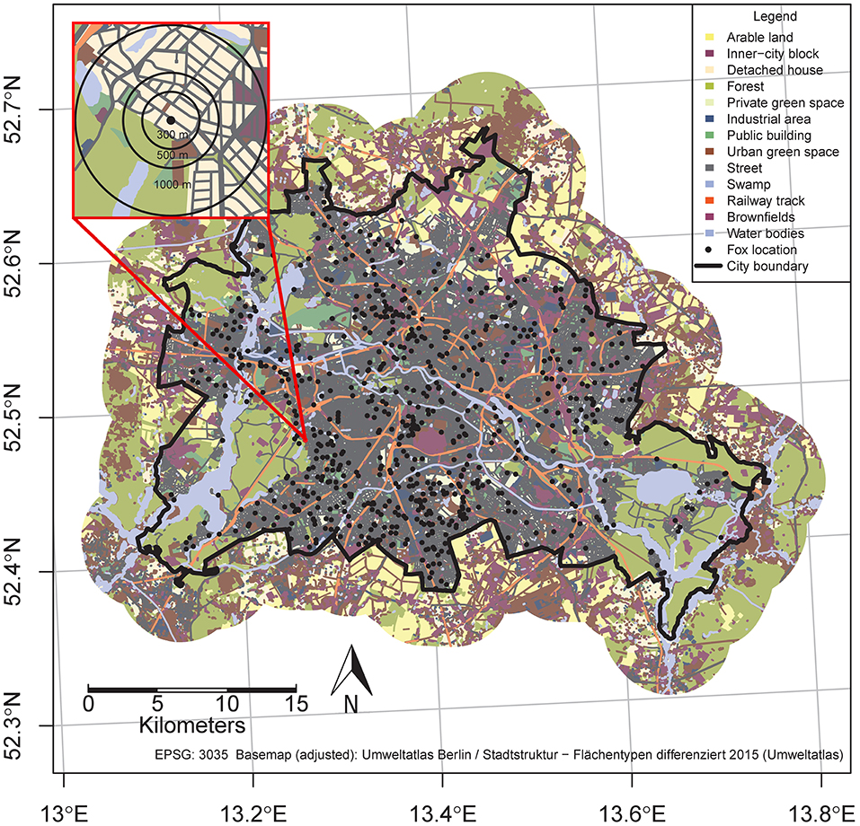
Figure 1. Study area and buffers to derive the landscape variables. The Figure shows different land use structures and the locations of the fox carcasses discovered between 2008 and 2013 in Berlin, Germany (black dots). The red framed detailed inset shows the area covered to analyze different spatial resolutions of the landscape variables; i.e., 28 ha (r = 300 m), 78 ha (r = 500 m), and 314 ha (r = 1,000 m) areas at the carcass finding locations.

Red Fox and Landscape Structure Data Acquisition and Preparation

Data management, analyses and Figures were done in R 3.4.1 (R Core Team, 2017) using the packages car 2.1-5 (Fox and Weisberg, 2011), corrplot 0.77 (Wei and Simko, 2016), DHARMa 0.1.5 (Hartig, 2017), data.table 1.10.4 (Dowle and Srinivasan, 2017), dismo 1.1-4 (Hijmans et al., 2017), dplyr 0.7.1 (Wickham et al., 2017a), effects 3.1-2 (Fox, 2003), GISTools 0.7-4 (Brunsdon and Chen, 2014), lattice 0.20-35 (Deepayan, 2008), lme4 1.1-13 (Bates et al., 2015), MuMIn 1.15.6 (Barton, 2016), pbapply 1.3-3 (Solymos and Zawadzki, 2017), raster 2.5-8 (Hijmans, 2017), readr 1.1.1 (Wickham et al., 2017b), rgdal 1.2-8 (Bivand et al., 2017), rgeos 0.3-23 (Bivand and Rundel, 2017), rpostgis 1.3.0 (Basille and Bucklin, 2017), RPostgreSQL 0.6-2 (Conway et al., 2017), sf 0.5-1 (Pebesma, 2017), sp 1.2-5 (Pebesma and Bivand, 2005; Bivand et al., 2013), tidyr 0.6.3 (Wickham and Henry, 2017), vegan 2.4-3 (Oksanen et al., 2017), viridis 0.4.0 (Garnier, 2017), zoo 1.8-0 (Zeileis and Grothendieck, 2005). Additionally we used SAGA GIS 4.0 and Gimp 2.8.

Red Fox Carcass Data

In total 813 fresh fox carcasses were collected between June 2008 and July 2013 in Berlin by the state laboratory of Berlin and Brandenburg. Berlin is a well-developed area with regular governmental street cleaning, thus the detection probability of carcasses across the whole area and throughout the study period was similar, and all found foxes are sent to the state laboratory (StrRein, 1979). Fox carcasses were found across the whole city except for forested areas where dead foxes remained hidden. We used various information associated with each carcass: finding location of the carcass, finding date, sex, age, cause of death (COD), and CDV serological status (i.e., presence or absence of CDV antibodies). The age of the foxes was determined based on dental appearance, and individuals were classified as “juvenile” (age <12 month) or “adult” (age >12 month) based on dentition changes and abrasion. To detect CDV antibodies in foxes the state laboratory used a direct immunofluorescence test (see Supplementary Material “S1 Description of lab methods”). A positive test result indicates seroconversion and thus previous exposure of the animal to CDV (Elnekave et al., 2016). All records providing an exact location (i.e., including the street name, the house number and postcode) were geocoded using the online tool GeoVisualizer (http://www.gpsvisualizer.com/geocoder/). Incomplete records (28 carcasses) were excluded, resulting in a final data set of 785 (see Data Sheet 1) carcasses. The specified GeoVisualizer source was “MapQuest Open” to obtain geographic WGS84 coordinates. In 2008 no age assessment was done by the laboratory, hence these data were excluded from all analyses demanding the incorporation of age.

Landscape Structure Data

To derive landscape variables we used land use maps of Berlin (SenSW, 2010) and Brandenburg (LfU, 2015). As all fox carcass records were within Berlin's administrative boundary we focused our analysis on the administrative boundary plus a 4 km buffer area to handle findings close to the administrative boundary. Both maps were intersected to obtain a topologically correct map of the study area (Berlin plus 4 km buffer zone from Brandenburg area). Based on this map we reclassified all occurring land use structures (752 categories) into 12 land use structures (see Figure 1) typical for urban areas and meaningful for urban foxes (Harris, 1977; Harris and Rayner, 1986; Janko et al., 2012; Börner, 2014): (1) arable land, (2) inner-city blocks (typical Berlin apartment houses), (3) forest, (4) private green space (gardens, allotments, camping sides), (5) industrial area (warehouses, power plants), (6) public building (schools, train stations), (7) urban green space (parks, botanical gardens), (8) streets, (9) detached houses (villa, leisure residence) (10) water bodies (rivers and lakes), (11) railway tracks (railway sidings and embankments), (12) brownfields covering unbuilt and anthropically unused areas.

Georeferenced carcass finding locations indicate the individual's death location; thus, we assigned a wider area (buffer) to each location to capture the possible land cover structures an individual might have used shortly before dying. In literature, home ranges—the area an animal uses during lifetime—of urban foxes differ from 25 to 78 ha (Harris, 1980; Gloor, 2002; Janko et al., 2012). Consequently, buffering was done at three different scales to identify the optimal spatial resolution of the landscape variables (Figure 1). We selected 28 ha, (300 m radius) and 78 ha (500 m radius) sized buffers reflecting literature findings (see above). In addition, a coarse resolution buffer of 314 ha (1,000 m radius) was selected due to preliminary results of an ongoing GPS telemetry study of foxes in Berlin (Sophia Kimmig, personal communication). All environmental variables (twelve land use structures and three landscape heterogeneity indices) were extracted for all locations of fox carcasses and at all spatial resolutions. We calculated the proportional share for each of the land use structures and calculated three landscape heterogeneity indices: (1) Shannon index, (2) Pielou's evenness, and (3) landscape structure richness to estimate land use heterogeneity for each location using the following formulas:

1) Richness: [S] is the count of land use structures at each location.

2) Shannon index: $H=-\sum _{i=1}^S{\rho }_{i}log(b){\rho }_i$ with [ρ_i] being the proportion of the land use structures[i], [S] the number of land use structures and [b] the base of the logarithm.

3) Pielou's evenness: $J=\frac{H}{log(S)}$ with [H] the Shannon index and [S] the richness.

Statistical Analysis, Model Selection and Evaluation of the Disease Seroprevalence Models

The workflow is pictured in Figure 2 and described below.

FIGURE 2

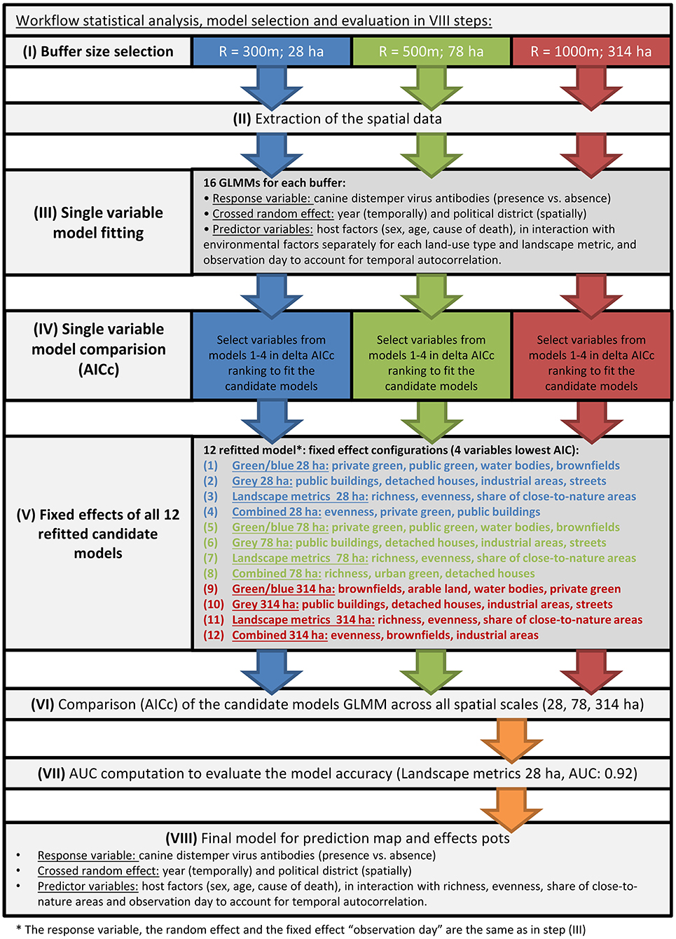
Figure 2. Workflow of the data analysis.

Fitting the Candidate Disease Seroprevalence Models

To find a final model predicting serostatus of CDV in foxes based on urban landscape structures and individual-level information, we compared sets of twelve candidate models (see Figure 2V) testing our hypotheses using multi-model inference based on AICc to maximize predictive power while controlling for model complexity (Symonds and Moussalli, 2011). We used Generalized Linear Mixed-Effects Models using the Laplacian approximation to the deviance (Bates et al., 2015) to correlate the landscape structure variables and CDV seroprevalence (presence vs. absence of CDV antibodies; seropositive = 1 vs. seronegative = 0) over the course of time, ignoring unlikely but possible method related errors (see Supplementary Material Description S1). To control for individual-level information effects, we used the covariates sex (female/male), age (juvenile/adult), cause of death (COD) (roadkill, n = 260 deliberately killed (no reason reported), n = 100 perished from disease or trauma, n = 149), their 3-way interaction and the random effect of administrative district (twelve levels). The random effect “administrative district” was a priori selected to capture social as well as historic developmental differences of the administrative districts in Berlin. The cause of death (COD) was included to control for the spatial pattern of roads in mortality while testing for the effect of landscape elements on CDV presence. For the level “perished from other disease or trauma” of the variable COD, the specific fatal disease was not reported. As age was not recorded in 2008, and occasionally not recorded afterwards, we had to drop 275 observations. From here onwards “whole study period” stands for the period from 2009 to 2013. Then we applied a four-fold partitioning to the data (n = 509) to obtain test (25%) and training (75%) datasets to assess the model's goodness of fit or discriminative ability, respectively (Area Under the Curve or AUC), leaving 382 observations to train the model. Assuming a necessary minimum of ten records for each factor level of a parameter the categorical fixed and random effects consumed 330 observations, leaving space to include four numeric landscape variables such as share of urban green space or landscape structure richness while avoiding overfitting. Thus, we created twelve ecologically different candidate models and compared the predictive power to obtain one final model offering the highest predictive power (see below). All numeric landscape variables were scaled around the mean and divided by standard deviation for easing model convergence during fitting.

Grouping and Selecting of Numeric Variables

We grouped all twelve landscape structure variables and the three landscape metrics by their ecological meaning and assigned them to one of the following ecological groups: (1) landscape metrics, (2) share of wildlife friendly area and (3) share of wildlife hostile area. More specifically, (1) “landscape metrics” consists of landscape structure richness, landscape structure Shannon index, landscape structure Pielou's evenness, (2) “blue/green infrastructure” of share of brownfields, private green space, water bodies, forest, railway tracks, urban green space, arable land and (3) “gray infrastructure” of share of industrial area, public buildings, detached houses, inner-city blocks, streets. Additionally we created (4) a “combined model”. The combined model was built by selecting the one landscape structure variable providing the highest predictive power out of the ecological groups one to three. To compare the predictive power of all landscape structure variables we fitted single-variable models (Figure 2III; formula in R language see Supplementary Material S2) at each spatial resolution (300, 500, and 1,000 m). The predictive power was assessed by AICc computation as described below.

Spatio-Temporal Autocorrelation, Nonlinearity and Correlation of Predictors

First, we tested for spatial and temporal autocorrelations in model residuals (Hartig, 2017). The administrative district was used as random effect and therefore a test for spatial autocorrelation non-significant. Second, we used the fixed effect observation day (the number of days since the first carcass was recorded) as integer covariate to handle temporal autocorrelation. The test for temporal autocorrelation became non-significant when observation day was included. Third, we fitted Generalized Additive Models (GAMs) to visually examine potential nonlinearity between predictor and response variable (see Supplementary Material Figure S3a). When the plots indicated some nonlinear second order relationships, we included the quadratic term of the given numeric predictor variable in each fitted model. Fourth, among the land use structures used in a given candidate model, no correlations were detected, but the Shannon index correlated with richness and evenness; thus we included only richness and evenness to handle collinearity (see Figure S5a).

Predictor Selection and Simplification of All Twelve Candidate Disease Prevalence Models

Here we applied a two-step procedure. First, we reduced the number of separate predictors within each of the three ecological groups of predictors (landscape metrics, share of wildlife friendly area and share of wildlife hostile area) by selecting the four most promising variables by fitting single predictor models (Figure 2IV, Supplementary Material Description S2, as described above but using only one numeric predictor) and assessing the predictive power of the resulting model using AICc (see Table S4a). To assess the change in predictive power due to the inclusion of numeric predictors, we compared all single predictor models to a null model (no fixed effects) and a model entailing only categorical predictors (individual-level variables as control). We selected the four predictors resulting in the lowest model AICc in each of the three ecological groups and tested Spearman's rank correlation coefficient (Wei and Simko, 2016) (see Figures S5a.1–S5a.12). The four best (lowest AICc) and not correlating predictors were refitted in one model entailing up to four numeric variables (Figure 2V). Additionally, we fitted a fourth combined model. The combined model was built by combining the one predictor providing the lowest model AICc of each ecological group and fitting all three within one model (see Table S6a candidate model list). These four models were fitted three times, each time using variables derived in another spatial resolution (28, 78, and 314 ha). Consequently, we got a set of twelve models.

Second, we applied a multi-model inference procedure (Figure 2VI), at it we retained the single predictor variables while the “variable importance” (Barton, 2016; number of models including the variable divided by the number models excluding the variable out of the best set of models, identified by delta AICc <10) was calculated for interactions and 2nd order polynomial; terms having a value below 0.6 were dropped to optimize the predictive power of each model (Barton, 2016) (final model configuration see Table 1). Across all twelve fitted models we compared AICc and selected the model with the lowest AICc. For this model we computed the AUC (Figure 2VII) and reported the model formula as final predictive model (Figure 2VIII).

TABLE 1

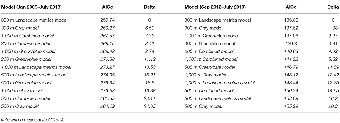
Table 1. Comparison of candidate models.

Modeling the Infection Period

Due to the longitudinal pattern of the recorded seropositive foxes (Figure S7) and because we had complete individual-level data (“age” variable) from foxes only since 2009 (Figure S8) when the disease had already started spreading, we could monitor the beginning of the disease spread only from April 2012 to July 2013. Hence, we modeled the second infection period again separately. To do so, we applied the whole procedure described above to a subset of the data gathered from April 2012 until July 2013 (see Supplementary Material S3b–S6b).

Identifying a Final Predictive Model, Assessing the Predictor Effects and Plotting of the Results

To obtain one final predictive model, we compared the results of the model assessments of both modeling approaches for (1) the whole period (2009–2013) and (2) the second infection period (2012–2013). The landscape metrics model at 28 ha spatial resolution was among the best (delta AIC <4) models for both analyses (see Table 1), i.e., the whole data analysis and the analysis restricted to the second infection period. Thus, we selected this model as final prediction model and reported the predictor configuration in Table 2. Statistical significance of the predictor variables retained during the multi-model inference procedure was derived by applying an ANOVA Type II (Fox and Weisberg, 2011). To visualize the interactions, we plotted the estimated effects of all sex/age categories and predicted the probability of finding seropositive individuals due to landscape variables in the area of of Berlin (Fox and Hong, 2009; Hijmans, 2017).

TABLE 2

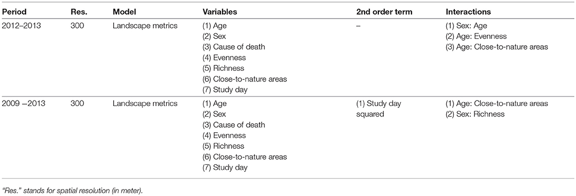
Table 2. Variable configuration of final prediction models (landscape metrics).

Assessing of the Temporal Pattern

To assess the longitudinal disease spread i.e., the effect of time on the relationship of CDV seroprevalence and landscape variables, we introduced the interaction of study day and all other predictors in our final model and assessed the significance applying an ANOVA Type II (Fox and Weisberg, 2011). Hence, the slope (serostatus vs. landscape structure) could vary during the course of time.

Prediction Map

Based on the final model for the whole period we predicted the probability of seropositivity across the whole area of Berlin. The prediction was based on the configuration of the landscape variables. The new values for each variable were obtained from raster images having a spatial resolution of 28 ha.

Results

CDV seropositive samples showed local clustering in different years (Figures 1, 3). The landscape variables showed distinct spatial distribution patterns such as high proportions of close-to-nature areas at the administrative boundary (Figure S9). In the analyzed fox samples the sex ratio was 0.8 (170 females vs. 214 males) and the ratio of adults to juveniles was similar in both sexes (~1.63) (Figure S10). For all analyzed individuals, the proportion of CDV seropositive animals was higher in adults of both sexes than in juveniles (Figure 4).

FIGURE 3

Figure 3. Spatiotemporal distribution of seropositive and seronegative fox carcasses in Berlin and the administrative districts (gray polygons).

FIGURE 4

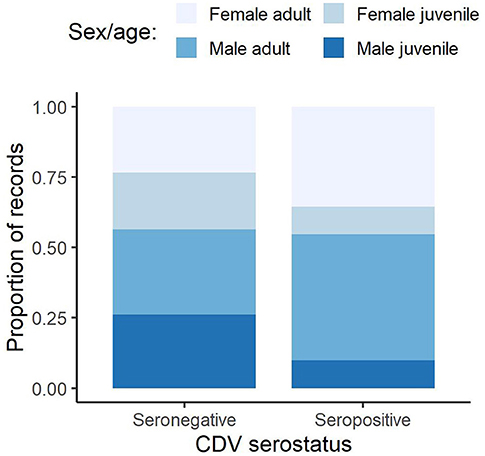
Figure 4. Relative proportions of CDV seropositive and negative foxes by sex and age.

The comparison of twelve candidate models across all ecological groups and spatial resolutions identified the landscape metrics model with variables derived at 28 ha (r = 300 m) resolution as the most powerful predictive model (Table 2). The result holds for the analysis of the whole study period from Jan 2009 to July 2013 (AUC = 0.92; delta AIC 2nd ranked model = 6.53) and the separately analyzed second infection period from April 2012 to July 2013 (AUC = 0.90; delta AIC 2nd ranked model = 1.93).

The ANOVA Type II of both models showed [see (1a) and (2) in Table 3, Table S11] (1) a significantly higher proportion of seropositive individuals among adults than juveniles (Chisq. 2009-2013 = 8.01; P 2009–2013 = 0.005, Chisq. 2012–2013 = 6.21; P 2012–2013 = 0.013), (2) that foxes killed in a car accident were least seropositive (Chisq. 2009–2013 = 39.20; P 2009–2013 = <0.001, Chisq. 2012–2013 = 19.07; P 2012–2013 = <0.001) and (3) that juveniles but not adults were more often seropositive when the share of close-to-nature habitats increased (Chisq. 2009–2013 = 8.43; P 2009–2013 = 0.004, Chisq. 2012–2013 = 7.01; P 2012–2013 = 0.008). The temporal pattern was a second order polynomial peaking at the beginning and the end of the study period when modeled from 2009 to 2013 (Chisq. Study day = 72.39; P Study day = <0.001; Chisq. Study day^∧2 = 78.23; P Study day^∧2 = <0.001) and a linear, increasing relationship when the second infection period—from 2012 to 2013—was modeled separately (Chisq. Study day = 17.81; P Study day = <0.001).

TABLE 3

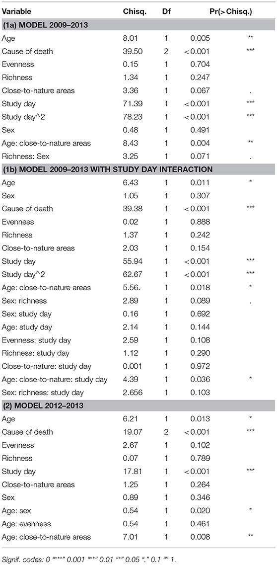
Table 3. ANOVA (Type II Wald chi square tests) table: landscape metrics models (1a) Jan 2009–July 2013, (1b) Jan 2009–July 2013 with study day interaction and (2) Apr 2012–July 2012.

Detailed view of the landscape structures driving spatial heterogeneity in CDV seroprevalence of urban foxes (Figure 5, Table 3, Table S11), showed that the number of positive juvenile foxes was lower with low shares of available close-to-nature habitats (Chisq. = 8.43, P = 0.004). In adult foxes this effect was not found (Chisq. = 3.36, P = 0.07). In females, CDV seroprevalence only tended to be higher with high richness of landscape structures (Chisq. = 3.25, P = 0.07, Table 3; Effect size = 0.61 ± SE 0.34, Table S11). The random effects showed slight differences (variance 0.029, standard deviation 0.17). Compared to fixed effects the random effects did not contribute substantially in explaining the variance of the data (marginal R² = 0.707, conditional R² = 0.709). Fitting the model with (A) and without (B) COD did not change the results. (A) No COD variable, Interaction age-suitable landscape: Estimate = 1.16, P = 0.003; (B) With COD variable, Interaction age-suitable landscape: Estimate = 1.23, P = 0.004. Moreover by dropping COD from the model the AUC changes from 0.92 to 0.88.

FIGURE 5

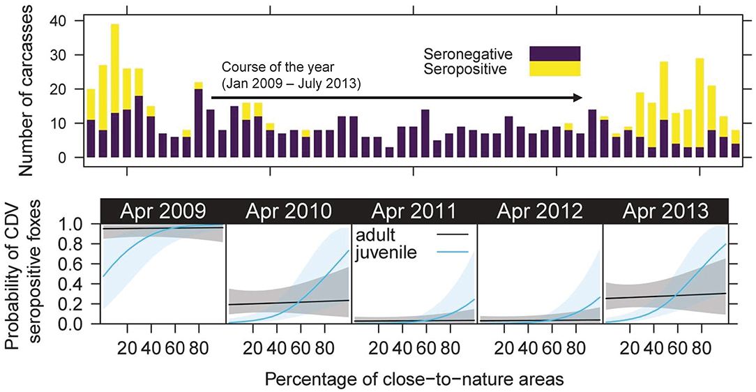
Figure 5. Landscape-seroprevalence relationship during the course of the study. Top: bar plot on showing the number of analyzed fox carcasses and the proportion of CDV seropositive foxes (raw data is presented in Figure S7, S8). Bottom: bottom row shows the modeled relationship of probability of CDV seroprevalence (y-axis) and the landscape structure richness in April of each analyzed year (x-axis).

The separate analysis of the reinfection period from 2012 to 2013 showed similar patterns but at a higher temporal resolution. Hence, it was possible to describe an interaction of sex and age (Chisq. = 0.54, P = 0.02), by which the number of seropositive juveniles exceeded the number of seropositive adults in males (Table S11). The remaining interaction of juveniles and evenness indicates that more seroprevalence positive foxes were found in more even landscapes (Table S11). Juvenile females responded somewhat delayed and at a lower level than the other classes of foxes (Table S11).

The added interaction of study day and all other predictors in our final model was significant for share of close-to-nature area (Chisq. = 4.39, P = 0.036). Hence, the effects of landscape structures changed over time, showing an increasingly steep slope during times when many foxes were found [see model (1b) in Table 3, Figure S12]. That means that seropositivity, which in juveniles most likely is infection, is significantly bound to the share of close-to-nature areas. The change over time in addition means that this represents the wave of infection spreading through these areas, and can be interpreted as a density-dependent process of transmission, because we can assume that fox density and contact is especially high in close-to-nature areas within the urban matrix. The prediction for the first infection peak had high errors, which were clearly lower during the second infection period (Figure S12).

The predicted time series (Figure 6) for adults and juveniles shows the temporal pattern very well, as the probability of being CDV seropositive was lowest in April 2011 in juveniles and adults. The probability for adults was almost even in space, but the probability for juveniles showed a clearly higher spatial heterogeneity with highest probabilities in the north, west and south-east of Berlin. The overall effect could be quantified, as the standard deviation across the map is much higher for juveniles compared to adults (e.g., in 2009: SD juveniles 0.29 vs. SD adults 0.05). The spatial patterns were strongest in times with a high seropositive rate (>50%) of the sampled individuals probabilities in 2009 and 2013.

FIGURE 6

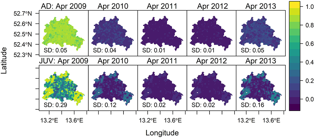
Figure 6. Map of predicted probability of CDV seropositive foxes from April 2009 to April 2013. The top row of plots shows adults (AD) the bottom row shows the pattern for juveniles (JUV). The color gradient indicates the probability of finding a seropositive fox based on landscape variables. SD stands for standard deviation and indicates the spatial variability of each prediction map.

The prediction map (Figure 7) shows areas with high or low seroprevalence in distinct landscape structures at a 28 ha (r = 300 m) spatial resolution. We identified areas close to large and homogeneous structures and water bodies as areas having the highest probability of CDV seropositive foxes (Figures 1, 7). In particular, forest edges close to water bodies showed probabilities above 0.8.

FIGURE 7

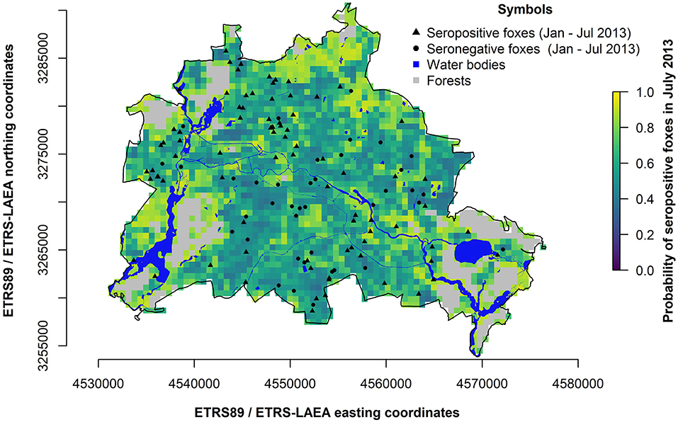
Figure 7. Map of predicted probability of CDV seropositive foxes (adults and juveniles) in Berlin during an epidemic in July 2013. The pixel color indicates the predicted seroprevalence based on landscape structures (bluish = low probability; yellowish = high probability; gray = forest areas, where no data was available). Dots represent fox carcass locations (red = seropositive, white = seronegative). Blue areas indicate water bodies. The black line is the administrative boundary of Berlin.

Discussion

We showed that a model including the share of close-to-nature habitats, landscape structure richness, landscape structure evenness, sex and age was the best in predicting CDV seroprevalence of urban foxes in Berlin. The probability to be CDV seropositive dropped by 66% for juvenile females (from 0.6 to 0.2) while the share of close-to-nature habitats dropped from 60 to 20%. Juvenile males showed a similar response, yet of lower magnitude. A landscape effect limited to juvenile foxes is likely, as CDV is known to infect mostly juveniles in several host species (Haas et al., 1996; Cleaveland et al., 2000), which then either recover and develop lifelong immunity (Greene, 2013) or die within a short period (Almberg et al., 2009). Hence, many seropositive adult foxes in this study were likely exposed to CDV as juveniles. This is supported by the fact that we observed a 30% higher CDV seroprevalence in adults than in juveniles, and that seroprevalence of adult foxes was independent of all tested landscape structure variables. Moreover, most foxes disperse in their second year of life (Harris and Trewhella, 1988), hence the majority of juveniles in our study (age <12 months) died in the areas where they lived their whole lives. The adults may have already dispersed, which most likely explains effects of the local landscape being restricted to juvenile foxes. Because of this specific infection process and dispersal behavior, similar results are to be expected when analyzing samples from foxes trapped alive instead of carcasses. Given the high effort required to capture foxes in Berlin (only 20 foxes could be captured in 4 years of continuous sampling effort as reported from another ongoing project), analyzing carcasses provides an interesting alternative in terms of sample size and hence power to detect spatial distribution patterns.

Harris and Trewhella (1988) showed that juvenile foxes born closer to the city center were older at time of death. Hence, they survived longer in an urban environment. They did not discuss this result, but several studies suggest increased fitness benefits in urban areas due to a high resource availability, a low hunting pressure and an absence of large predators as possible explanations (Cavallini, 1996; Contesse et al., 2004; Börner, 2014). Here, we reveal that juvenile foxes in areas with high shares of built-up areas had a lower exposure to CDV. Consequently, the absence of diseases or the reduced risk of disease transmission due to spatial isolation may be another factor contributing to increase the fitness of foxes in strongly urbanized areas.

We showed that areas providing low shares of close-to-nature habitats harbor less locally seroconverted foxes, i.e., juveniles younger than 1 year. A decreasing share of close-to-nature areas corresponds to an increasing share of physical barriers. This result may thus indicate that artificial physical barriers could have reduced contacts among foxes and between foxes and other species in our study area, and therefore impaired CDV transmission. Such an effect of a landscape barrier, e.g., a river, separating not only populations but also impairing disease transmission, was shown for rabies in raccoons (Rees et al., 2008). This is a pattern well-grounded in the literature, as contact rate is a major driver of disease spread in directly transmitted diseases of mammals (Brearley et al., 2013). In addition, urban areas are resource-rich habitats supporting generalist mammals such as foxes (Cavallini, 1996; Contesse et al., 2004; Börner, 2014). In other terms, in resource rich urban areas an increasing degree of isolation might create refuge habitats preventing disease spillover from other individuals or other species for generalist species such as foxes. In the future, intra- and inter-specific disease transmission within these habitats needs to be addressed in detail to identify mechanistic relationships.

Rentería-Solís et al. (2014) showed that foxes and raccoons are infected by closely related CDV strains. Interestingly, raccoons use predominantly close-to-nature habitats such as forests (Frantz et al., 2005). A major CDV epidemic of Berlin's raccoon population occurred between December 2012 and May 2013 (Rentería-Solís et al., 2014), simultaneously with the second epidemic of Berlin's foxes (December 2012–May 2013). We did not investigate interspecies transmission, but these findings raise concerns about the risks of interspecific transmission of CDV, and whether or not raccoons and foxes can infect each other. Interspecific transmission is possible, because it is known that CDV infects a wide and increasing range of host species (Appel and Summers, 1995; Roelke-Parker et al., 1996; Harder and Osterhaus, 1997; Deem et al., 2000; Frölich et al., 2000; Pomeroy et al., 2008; Beineke et al., 2015; Martinez-Gutierrez and Ruiz-Saenz, 2016) and spontaneous transmission to novel host species is known to occur (Harder and Osterhaus, 1997; Martinez-Gutierrez and Ruiz-Saenz, 2016). Spontaneous interspecific transmission between foxes and raccoons during the second infection period would explain the areal distribution of seropositive foxes compared to the patchy pattern during the first CDV spreading period in Berlin's foxes in 2008. Agonistic interactions among dogs (Canis familiaris) and indian foxes (Vulpes bengalensis) are assumed to be a major driver of transmission of virulent diseases such as CDV, as both species can host the same viruses and viral strains (Belsare et al., 2014). Moreover, CDV can persist for several days without a host in cold environments (Deem et al., 2000). Whether consecutive visits of foxes and/or raccoons in the same area lead to additional inter- or intra-specific infections is yet unknown and hard to prove in the field. However, surveillance and disease control actions targeting CDV in urban landscapes must include at least foxes, raccoons, and pet dogs, if not many more unknown host species, and such actions should be tailored to the home range of all hosts.

The observed effects of the covariate “age” is in line with our expectation. Whereas seropositive adults are most likely individuals that got infected as juveniles, a large share of seropositive juveniles may represent locally seroconverted and newly infected individuals. This applied especially well to the second infection period (2012 to 2013), as we did not record any incidence of CDV in foxes between mid-2010 and mid-2012. Most juveniles disperse in their second year (Harris and Trewhella, 1988); a gap of 2 years should be sufficient to underpin the assumption that seropositive juveniles recorded between late 2012 and mid 2013 were infected locally.

Finding the optimal spatial resolution to study patterns on the ecosystem level is challenging but important to understand and interpret emerging patterns, as there is not one spatial resolution suiting all ecological phenomena (Levin, 1992). However, few studies (13 out of 98) assessed the impact of multiple spatial resolutions on disease spread within the same study (Meentemeyer et al., 2012). We showed that landscape variables derived in a circle covering 28 ha (radius 300 m) around the carcass finding places provided the highest predictive power compared with coarser spatial resolutions (78 ha or 314 ha). Home ranges of foxes vary between 25 ha and 78 ha in urban areas (Harris, 1980; Gloor, 2002; Janko et al., 2012). Rural foxes (Henry et al., 2005) and preliminary results of a telemetry study on movement of urban foxes in Berlin point on larger home ranges of up to 310 ha (Sophia Kimmig, personal communication). Thus, the selected resolutions 28 ha (300 m radius), 78 ha (500 m radius), and 314 ha (1,000 m radius) covered the known variation of home ranges in foxes. Finding the highest resolution as most informative is in line with the literature as environmental data at high spatial resolution (very precise) is most effective to capture the occurring spatial heterogeneity and therefore predicts animal distribution well (Rocchini et al., 2015). Linking the home range size and disease distribution does come naturally, as the home range limits the physical presence and thus the spatial distribution in which an individual may distribute any sort of disease (Pleydell et al., 2004). Here, using previous knowledge about the home range size to determine the studied spatial scale improved the predictive power. Consequently, we demonstrated that linking home range size and spatial resolution of environmental parameters is an effective method to improve the power of a predictive model.

The significant interaction of study day and close-to-nature areas for juvenile foxes indicates that the landscape effect is not persistent per se. The magnitude of this effect was stronger when disease incidence and host density were highest. Indeed, the strongest effects of the landscape were recorded in 2009 and 2013, when most individuals as well as the highest CDV seroprevalence were recorded. This result is in line with theory, as high wildlife densities increase intra- and inter-specific disease transmission (Cleaveland et al., 2000; Ditchkoff et al., 2006; Almberg et al., 2009). Thus, if a host carries a disease into an area with high population density—as we expect in our study region in 2009 —the disease might spread quickly in the areas with the highest individual densities. On the other hand, if population density and contact rates are low disease transmission may not occur by direct transmissions, but indirectly through traces in the landscape as individuals with adjacent home ranges visit the same places occasionally. This seems applicable to territorial urban foxes as home ranges overlap slightly (Harris, 1980; Adkins and Stott, 1998) and determine the individual occurrence and the spatial distribution (Pleydell et al., 2004). However, such a theory is speculative until disease transmission, population density and landscape structure are all analyzed simultaneously at a high temporal resolution in one area. We could not conduct such an analysis as we lack data on population density and a high spatiotemporal resolution. Such studies are very difficult to conduct but important to identify causal relationships to understand how disease outbreaks shape the spatial distribution of urban mammals, as mentioned in the literature (Baker et al., 2004). Understanding disease spread is increasingly important as the number of zoonotic diseases from wild animals tend to increase (Bengis et al., 2004). Moreover, proximity of wildlife and humans make zoonoses or exchange of diseases among pets and wildlife more likely, particularly in urban areas (Adkins and Stott, 1998; Ditchkoff et al., 2006). To understand and manage disease spread, environmental effects cannot be neglected. Especially, as diseases such as CDV can persist for several hours/days without a host in the environment (Deem et al., 2000). In urban environments, close-to-nature areas in direct proximity to water bodies are typical animal dispersal corridors and human recreation areas. Predictive models, as the one presented here, help to identify specific places having a high infection risk independent of a current epidemic. We created a prediction map based on landscape structure indicating areas of high probability of finding a seropositive fox. Such areas were situated close to water bodies and large continuous close-to-nature habitats, the common dispersal corridors of urban mammals (Beninde et al., 2015). Hence, surveillance and disease control actions such as vaccination should be focused on individuals inhabiting these areas. Predictive models as the one presented here are of paramount importance to guide landscape management and to identify areas supporting a high CDV risk. Preventive actions may be necessary, as rapidly spreading diseases such as CDV are hardly manageable when locally spreading (Stubbe, 1980; Appel and Summers, 1995; Harder and Osterhaus, 1997; Bradley and Altizer, 2007; Williams and Barker, 2008; Rentería-Solís et al., 2014).

The importance of the urban structural landscape variables for assessing the risk of finding seropositive juvenile animals, i.e., the potential disease spreaders, needs to be validated by application to fully independent data of another study region to prove transferability, as responses of host-pathogen systems to landscape effects are very diverse and not consistent across species and regions (Brearley et al., 2013). Moreover, predictive power and accuracy may be further increased by incorporating data about population density, resource distribution and individual fitness. While the latter seems to be very difficult to assess, incorporating the first two may be possible in due time as high-throughput DNA sequencing, camera trapping and remote sensing rapidly becomes increasingly affordable and highly precise (Bush et al., 2017; Pettorelli et al., 2017; Wegmann, 2017). Despite lacking these potential methodological improvements, we could still demonstrate here that an increase of built-up areas by 40% may reduce the probability of juvenile foxes to experience CDV within their first year of age by 66%, a result suggesting a lower CDV infection risk in strongly urbanized areas.

Data Availability Statement

The red fox dataset analyzed for this study can be found in the supplementary material.

Author Contributions

SK-S, BK, and KB conceived the study. SK-S, BK, and PG designed it. PG and SK analyzed data and drafted the manuscript. AA and UW screened the samples. SB and LM helped defining the disease states for the statistical analyses, all authors contributed to the writing of the manuscript.

Funding

The work was funded by the German Federal Ministry of Education and Research BMBF within the Collaborative Project Bridging in Biodiversity Science-BIBS (funding number 01LC1501A-H). SB and LM were supported by the Deutsche Forschungsgemeinschaft (DFG grants EA 5/3-1, KR4266/2-1).

Conflict of Interest Statement

The authors declare that the research was conducted in the absence of any commercial or financial relationships that could be construed as a potential conflict of interest.

Acknowledgments

We thank all the helping hands involved in collecting fox carcasses, handing them over to the Landeslabor Berlin-Brandenburg or supporting the processing of samples. Further, we thank our colleagues for feedback and lively discussion on the subject and the reviewers.

Supplementary Material

The Supplementary Material for this article can be found online at: https://www.frontiersin.org/articles/10.3389/fevo.2018.00136/full#supplementary-material

References

Adkins, C. A., and Stott, P. (1998). Home ranges, movements and habitat associations of red foxes Vulpes vulpes in suburban Toronto, Ontario, Canada. J. Zool. 244, 335–346. doi: 10.1111/j.1469-7998.1998.tb00038.x

CrossRef Full Text | Google Scholar

Almberg, E. S., Mech, L. D., Smith, D. W., Sheldon, J. W., and Crabtree, R. L. (2009). A serological survey of infectious disease in Yellowstone National Park's canid community. PLoS ONE 4:e7042. doi: 10.1371/journal.pone.0007042

PubMed Abstract | CrossRef Full Text | Google Scholar

Appel, M. J., and Summers, B. A. (1995). Pathogenicity of morbilliviruses for terrestrial carnivores. Vet. Microbiol. 44, 187–191.

PubMed Abstract | Google Scholar

Baker, P., Funk, S., Harris, S., Newman, T., Saunders, G., and White, P. (2004). “The impact of human attitudes on the social and spatial organization of urban foxes (Vulpes vulpes) before and after an outbreak of sarcoptic mange,” in Proceedings of the 4th International Symposium on Urban Wildlife Conservation, eds W. W. Shaw, L. K. Harris, and L. VanDruff (Tucson, AZ: The University of Arizona).

Google Scholar

Baker, P. J., Robertson, C. P. J., Funk, S. M., and Harris, S. (1998). Potential fitness benefits of group living in the red fox, Vulpes vulpes. Anim. Behav. 56, 1411–1424. doi: 10.1006/anbe.1998.0950

PubMed Abstract | CrossRef Full Text | Google Scholar

Barton, K. (2016). MuMIn: Multi-Model Inference. Available online at: https://CRAN.R-project.org/package=MuMIn

Basille, M., and Bucklin, D. (2017). Rpostgis: R Interface to a ‘PostGIS’ Database. Available online at: https://CRAN.R-project.org/package=rpostgis

Bates, D., Mächler, M., Bolker, B., and Walker, S. (2015). Fitting linear mixed-effects models using lme4. J. Stat. Softw. 67, 1–48. doi: 10.18637/jss.v067.i01

CrossRef Full Text | Google Scholar

Beineke, A., Baumgärtner, W., and Wohlsein, P. (2015). Cross-species transmission of canine distemper virus—an update. One Health 1, 49–59. doi: 10.1016/j.onehlt.2015.09.002

PubMed Abstract | CrossRef Full Text | Google Scholar

Belsare, A. V., Vanak, A. T., and Gompper, M. E. (2014). Epidemiology of viral pathogens of free-ranging dogs and Indian foxes in a human-dominated landscape in central India. Transbound. Emerg. Dis. 61 (Suppl. 1), 78–86. doi: 10.1111/tbed.12265

PubMed Abstract | CrossRef Full Text | Google Scholar

Bengis, R. G., Leighton, F. A., Fischer, J. R., Artois, M., Mörner, T., and Tate, C. M. (2004). The role of wildlife in emerging and re-emerging zoonoses. Rev. Sci. Tech. 23, 497–511. doi: 10.20506/rst.23.2.1498

PubMed Abstract | CrossRef Full Text | Google Scholar

Beninde, J., Veith, M., and Hochkirch, A. (2015). Biodiversity in cities needs space: a meta-analysis of factors determining intra-urban biodiversity variation. Ecol. Lett. 18, 581–592. doi: 10.1111/ele.12427

PubMed Abstract | CrossRef Full Text | Google Scholar

Bivand, R. S., Keitt, T., and Rowlingson, B. (2017). rgdal: Bindings for the ‘Geospatial’ Data Abstraction Library. R package version 1.2-8. Available online at: https://CRAN.R-project.org/package=rgdal

Bivand, R. S., Pebesma, E., and Gomez-Rubio, V. (2013). Applied Spatial Data Analysis With R, Second Edition. NY: Springer. Available online at: http://www.asdar-book.org/

Google Scholar

Bivand, R. S., and Rundel, C. (2017). rgeos: Interface to Geometry Engine - Open Source (‘GEOS’). R package Version 0.3-23. Available online at: https://CRAN.R-project.org/package=rgeos

Börner, K. (2014). Untersuchungen zur Raumnutzung des Rotfuchses, Vulpes vulpes (L., 1758), in verschieden anthropogen beeinflussten Lebensräumen Berlins und Brandenburgs. [dissertation]. Berlin: Humboldt-Universität zu Berlin.

Bradley, C. A., and Altizer, S. (2007). Urbanization and the ecology of wildlife diseases. Trends Ecol. Evol. 22, 95–102. doi: 10.1016/j.tree.2006.11.001

PubMed Abstract | CrossRef Full Text | Google Scholar

Brearley, G., Rhodes, J., Bradley, A., Baxter, G., Seabrook, L., Lunney, D., et al. (2013). Wildlife disease prevalence in human-modified landscapes. Biol. Rev. Camb. Philos. Soc. 88, 427–442. doi: 10.1111/brv.12009

PubMed Abstract | CrossRef Full Text | Google Scholar

Brunsdon, C., and Chen, H. (2014). GISTools: Some further GIS capabilities for R. R package Version 0.7-4. Available online at: https://CRAN.R-project.org/package=GISTools

Bush, A., Sollmann, R., Wilting, A., Bohmann, K., Cole, B., Balzter, H., et al. (2017). Connecting earth observation to high-throughput biodiversity data. Nat. Ecol. Evol. 1:176. doi: 10.1038/s41559-017-0176

PubMed Abstract | CrossRef Full Text | Google Scholar

Cavallini, P. (1996). Variation in the social system of the red fox. Ethol. Ecol. Evol. 8, 323–342. doi: 10.1080/08927014.1996.9522906

CrossRef Full Text | Google Scholar

Cleaveland, S., Appel, M. G., Chalmers, W. S., Chillingworth, C., Kaare, M., and Dye, C. (2000). Serological and demographic evidence for domestic dogs as a source of canine distemper virus infection for Serengeti wildlife. Vet. Microbiol. 72, 217–227. doi: 10.1016/S0378-1135(99)00207-2

PubMed Abstract | CrossRef Full Text | Google Scholar

Contesse, P., Hegglin, D., Gloor, S., Bontadina, F., and Deplazes, P. (2004). The diet of urban foxes (Vulpes vulpes) and the availability of anthropogenic food in the city of Zurich, Switzerland. Mamm. Biol. Zeitschrift fur Saugetierkunde 69, 81–95. doi: 10.1078/1616-5047-00123

CrossRef Full Text | Google Scholar

Conway, J., Eddelbuettel, D., Nishiyama, T., Prayaga, S. K., and Tiffin, N. (2017). RPostgreSQL: R Interface to the ‘PostgreSQL’ Database System. R package version 0.6-2. Available online at: https://CRAN.R-project.org/package=RPostgreSQL

Damien, B. C., Martina, B. E., Losch, S., Mossong, J., Osterhaus, A. D., and Muller, C. P. (2002). Prevalence of antibodies against canine distemper virus among red foxes in Luxembourg. J. Wildl. Dis. 38, 856–859. doi: 10.7589/0090-3558-38.4.856

PubMed Abstract | CrossRef Full Text | Google Scholar

Deem, S., Spelman, L., Yates, R., and Montali, R. (2000). Canine distemper in terrestrial carnivores: a review. J. Zoo. Wildl. Med. 31, 441–451. doi: 10.1638/1042-7260(2000)031[0441:cditca]2.0.co;2

PubMed Abstract | CrossRef Full Text | Google Scholar

Deepayan, S. (2008). Lattice: Multivariate Data Visualization with R. New York, NY: Springer.

Google Scholar

Ditchkoff, S. S., Saalfeld, S. T., and Gibson, C. J. (2006). Animal behavior in urban ecosystems: modifications due to human-induced stress. Urban Ecosyst. 9, 5–12. doi: 10.1007/s11252-006-3262-3

CrossRef Full Text | Google Scholar

Dowle, M., and Srinivasan, A. (2017). data.table: Extension of ‘data.frame’. R package version 1.10.4. Available online at: https://CRAN.R-project.org/package=data.table

Dugord, P.-A., Lauf, S., Schuster, C., and Kleinschmit, B. (2014). Land use patterns, temperature distribution, and potential heat stress risk? The case study Berlin, Germany. Comput. Environ. Urban Syst. 48, 86–98. doi: 10.1016/j.compenvurbsys.2014.07.005

CrossRef Full Text | Google Scholar

Elnekave, E., King, R., van Maanen, K., Shilo, H., Gelman, B., Storm, N., et al. (2016). Seroprevalence of foot-and-mouth disease in susceptible wildlife in Israel. Front. Vet. Sci. 3:32. doi: 10.3389/fvets.2016.00032

PubMed Abstract | CrossRef Full Text | Google Scholar

Fox, J. (2003). Effect displays in r for generalised linear models. J. Stat. Softw. 8, 1–27. doi: 10.18637/jss.v008.i15

CrossRef Full Text | Google Scholar

Fox, J., and Hong, J. (2009). Effect displays inrfor multinomial and proportional-odds logit models: extensions to theeffectspackage. J. Stat. Softw. 32, 1–24. doi: 10.18637/jss.v032.i01

CrossRef Full Text | Google Scholar

Fox, J., and Weisberg, S. (2011). An R Companion to Applied Regression, Second Edition. Thousand Oaks, CA: Sage Publications, Inc.

Google Scholar

Frantz, A. C., Cyriacks, P., and Schley, L. (2005). Spatial behaviour of a female raccoon (Procyon lotor) at the edge of the species' European distribution range. Eur. J. Wildl. Res. 51, 126–130. doi: 10.1007/s10344-005-0091-2

CrossRef Full Text | Google Scholar

Frölich, K., Czupalla, O., Haas, L., Hentschke, J., Dedek, J., and Fickel, J. (2000). Epizootiological investigations of canine distemper virus in free-ranging carnivores from Germany. Vet. Microbiol. 74, 283–292. doi: 10.1016/S0378-1135(00)00192-9

PubMed Abstract | CrossRef Full Text | Google Scholar

Garnier, S. (2017). viridis: Default Color Maps from ‘matplotlib’. R package version 0.5.1. Available online at: https://CRAN.R-project.org/package=viridis

Gloor, S. (2002). The Rise of Urban Foxes (Vulpes Vulpes) in Switzerland and Ecological and Parasitological Aspects of a Fox Population in the Recently Colonised City of Zurich, dissertation, Universität Zürich, Zürich.

Greene, C. E. (2013). Infectious Diseases of the Dog and Cat. St. Louis, MO: Elsevier

Google Scholar

Haas, L., Hofer, H., East, M., Wohlsein, P., Liess, B., and Barrett, T. (1996). Canine distemper virus infection in Serengeti spotted hyenas. Vet. Microbiol. 49, 147–152.

PubMed Abstract | Google Scholar

Harder, T. C., and Osterhaus, A. D. (1997). Canine distemper virus–a morbillivirus in search of new hosts? Trends Microbiol. 5, 120–124. doi: 10.1016/S0966-842X(97)01010-X

PubMed Abstract | CrossRef Full Text | Google Scholar

Harris, S. (1977). Distribution, habitat utilization and age structure of a suburban fox (Vulpes vulpes) population. Mamm. Rev. 7, 25–38. doi: 10.1111/j.1365-2907.1977.tb00360.x

CrossRef Full Text | Google Scholar

Harris, S. (1980). “Home ranges and patterns of distribution of foxes (Vulpes vulpes) in an urban area, as revealed by radio tracking,” in A Handbook on Biotelemetry and Radio Tracking (Oxford), 685–690.

Google Scholar

Harris, S. (1981). The food of suburban foxes (Vulpes vulpes), with special reference to London. Mamm. Rev. 11, 151–168. doi: 10.1111/j.1365-2907.1981.tb00003.x

CrossRef Full Text | Google Scholar

Harris, S., and Baker, P. (2001). Urban Foxes. Essex: Whittet Books Ltd.

Google Scholar

Harris, S., and Rayner, J. M. V. (1986). Models for predicting urban fox (Vulpes vulpes) numbers in british cities and their application for rabies control. J. Anim. Ecol. 55, 593–603. doi: 10.2307/4741

CrossRef Full Text | Google Scholar

Harris, S., and Smith, G. C. (1987). Demography of two urban fox (Vulpes vulpes) populations. J. Appl. Ecol. 24, 75–86. doi: 10.2307/2403788

CrossRef Full Text | Google Scholar

Harris, S., and Trewhella, W. J. (1988). An analysis of some of the factors affecting dispersal in an urban fox (Vulpes vulpes) population. J. Appl. Ecol. 25:409. doi: 10.2307/2403833

CrossRef Full Text | Google Scholar

Hartig, F. (2017). Residual Diagnostics for Hierarchical (Multi-Level / Mixed) Regression Models [R package DHARMa version 0.1.5]. (Accessed December 1, 2017) Available online at: https://CRAN.R-project.org/package=DHARMa

Hassell, J. M., Begon, M., Ward, M. J., and Févre, E. M. (2016). Urbanization and disease emergence: dynamics at the wildlife-livestock-human interface. Trends Ecol. Evol. 32, 55–67. doi: 10.1016/j.tree.2016.09.012

PubMed Abstract | CrossRef Full Text | Google Scholar

Henry, C., Poulle, M.-L., and Roeder, J.-J. (2005). Effect of sex and female reproductive status on seasonal home range size and stability in rural red foxes (Vulpes vulpes). Écoscience 12, 202–209. doi: 10.2980/i1195-6860-12-2-202.1

CrossRef Full Text | Google Scholar

Hentschke, J. (1995). Staupe und Parvovirose - ein Problem in der Grossstadt? Prakt. Tierarzt 8, 695–703.

Google Scholar

Hijmans, R. J. (2017). raster: Geographic Data Analysis and Modeling. Available online at: https://CRAN.R-project.org/package=raster

Hijmans, R. J., Phillips, S., Leathwick, J., and Elith, J. (2017). dismo: Species Distribution Modeling. R package version 1.1-4. Available online at: https://CRAN.R-project.org/package=dismo

House, T., and Keeling, M. J. (2011). Insights from unifying modern approximations to infections on networks. J. R. Soc. Interface 8, 67–73. doi: 10.1098/rsif.2010.0179

PubMed Abstract | CrossRef Full Text | Google Scholar

Janko, C., Schröder, W., Linke, S., and König, A. (2012). Space use and resting site selection of red foxes (Vulpes vulpes) living near villages and small towns in Southern Germany. Acta Theriol. 57, 245–250. doi: 10.1007/s13364-012-0074-0

CrossRef Full Text | Google Scholar

Johnson, M. T. J., and Munshi-South, J. (2017). Evolution of life in urban environments. Science 358:eaam8327. doi: 10.1126/science.aam8327

PubMed Abstract | CrossRef Full Text | Google Scholar

Kauffman, M. J., and Jules, E. S. (2006). Heterogeneity shapes invasion: host size and environment influence susceptibility to a nonnative pathogen. Ecol. Appl. 16, 166–175. doi: 10.1890/05-0211

PubMed Abstract | CrossRef Full Text | Google Scholar

Kimoto, T. (1986). In vitro and in vivo properties of the virus causing natural canine distemper encephalitis. J. Gen. Virol. 67(Pt 3), 487–503. doi: 10.1099/0022-1317-67-3-487

CrossRef Full Text

Kramer-Schadt, S., Fernández, N., Eisinger, D., Grimm, V., and Thulke, H.-H. (2009). Individual variations in infectiousness explain long-term disease persistence in wildlife populations. Oikos 118, 199–208. doi: 10.1111/j.1600-0706.2008.16582.x

CrossRef Full Text | Google Scholar

Lauf, S., Haase, D., and Kleinschmit, B. (2014). Linkages between ecosystem services provisioning, urban growth and shrinkage – A modeling approach assessing ecosystem service trade-offs. Ecol. Indic. 42, 73–94. doi: 10.1016/j.ecolind.2014.01.028

CrossRef Full Text | Google Scholar

Levin, S. A. (1992). The problem of pattern and scale in ecology: the robert h. macarthur award lecture. Ecology 73, 1943–1967. doi: 10.2307/1941447

CrossRef Full Text | Google Scholar

LfU (2015). Kartierung von Biotopen, Gesetzlich Geschützten Biotopen (§ 30 Bnatschg Und § 18 Bbgnatschag) Und Ffh-Lebensraumtypen im Land Brandenburg. Available online at: http://www.mlul.brandenburg.de/lua/gis/biotope_lrt.zip

Lloyd-Smith, J. O., Schreiber, S. J., Kopp, P. E., and Getz, W. M. (2005). Superspreading and the effect of individual variation on disease emergence. Nature 438, 355–359. doi: 10.1038/nature04153

PubMed Abstract | CrossRef Full Text | Google Scholar

Marescot, L., Benhaiem, S., Gimenez, O., Hofer, H., Lebreton, J. D., Olarte-Castillo, X. A., et al. (2018). Social status mediates the fitness costs of infection with canine distemper virus in Serengeti spotted hyenas. Funct. Ecol. 32, 1237–1250. doi: 10.1111/1365-2435.13059

CrossRef Full Text | Google Scholar

Martinez-Gutierrez, M., and Ruiz-Saenz, J. (2016). Diversity of susceptible hosts in canine distemper virus infection: a systematic review and data synthesis. BMC Vet. Res. 12:78. doi: 10.1186/s12917-016-0702-z

PubMed Abstract | CrossRef Full Text | Google Scholar

Meentemeyer, R. K., Haas, S. E., and Václavík, T. (2012). Landscape epidemiology of emerging infectious diseases in natural and human-altered ecosystems. Annu. Rev. Phytopathol. 50, 379–402. doi: 10.1146/annurev-phyto-081211-172938

PubMed Abstract | CrossRef Full Text | Google Scholar

Oksanen, J., Blanchet, F. G., Friendly, M., Kindt, R., Legendre, P., McGlinn, D., et al. (2017). vegan: Community Ecology Package. R package version 2.4-3. Available online at: https://CRAN.R-project.org/package=vegan

Parris, K. M. (2016). Ecology of Urban Environments. West Sussex: Wiley-Blackwell.

Google Scholar

Pebesma, E. (2017). sf: Simple Features for R. R package version 0.5-1. Available online at: https://CRAN.R-project.org/package=sf

Pebesma, E. J., and Bivand, R. S. (2005). Classes and Methods for Spatial Data in R. R News 5. Available online at: https://cran.r-project.org/doc/Rnews/

Pettorelli, N., Schulte to Bühne, H., Tulloch, A., Dubois, G., Macinnis-Ng, C., Queirós, A. M., et al. (2017). Satellite remote sensing of ecosystem functions: opportunities, challenges and way forward. Remote Sensing Ecol. Conserv. 4, 71–93. doi: 10.1002/rse2.59

CrossRef Full Text | Google Scholar

Pleydell, D. R., Raoul, F., Tourneux, F., Danson, F. M., Graham, A. J., Craig, P. S., et al. (2004). Modelling the spatial distribution of Echinococcus multilocularis infection in foxes. Acta Trop. 91, 253–265. doi: 10.1016/j.actatropica.2004.05.004

PubMed Abstract | CrossRef Full Text | Google Scholar

Pomeroy, L. W., Bjørnstad, O. N., and Holmes, E. C. (2008). The evolutionary and epidemiological dynamics of the paramyxoviridae. J. Mol. Evol. 66, 98–106. doi: 10.1007/s00239-007-9040-x

PubMed Abstract | CrossRef Full Text | Google Scholar

Prange, S., Gehrt, S. D., and Wiggers, E. P. (2004). Influences of anthropogenic resources on raccoon (Procyon lotor) movements and spatial distribution. J. Mammal. 85, 483–490. doi: 10.1644/1383946

CrossRef Full Text | Google Scholar

R Core Team, (2017). R: A language and environment for statistical computing. Vienna: R Foundation for Statistical Computing. Available online at: https://www.R-project.org/

Rees, E. E., Pond, B. A., Cullingham, C. I., Tinline, R., Ball, D., Kyle, C. J., et al. (2008). Assessing a landscape barrier using genetic simulation modelling: implications for raccoon rabies management. Prev. Vet. Med. 86, 107–123. doi: 10.1016/j.prevetmed.2008.03.007

PubMed Abstract | CrossRef Full Text | Google Scholar

Rentería-Solís, Z., Förster, C., Aue, A., Wittstatt, U., Wibbelt, G., and König, M. (2014). Canine distemper outbreak in raccoons suggests pathogen interspecies transmission amongst alien and native carnivores in urban areas from Germany. Vet. Microbiol. 174, 50–59. doi: 10.1016/j.vetmic.2014.08.034

PubMed Abstract | CrossRef Full Text | Google Scholar

Riley, S. P. D., Sauvajot, R. M., Fuller, T. K., York, E. C., Kamradt, D. A., Bromley, C., et al. (2003). Effects of urbanization and habitat fragmentation on bobcats and coyotes in Southern California. Conserv. Biol. 17, 566–576. doi: 10.1046/j.1523-1739.2003.01458.x

CrossRef Full Text | Google Scholar

Rocchini, D., Boyd, D. S., Féret, J.-B., Foody, G. M., He, K. S., Lausch, A., et al. (2015). Satellite remote sensing to monitor species diversity: potential and pitfalls. Remote Sens. Ecol. Conserv. 2, 25–36. doi: 10.1002/rse2.9

CrossRef Full Text | Google Scholar

Roelke-Parker, M. E., Munson, L., Packer, C., Kock, R., Cleaveland, S., Carpenter, M., et al. (1996). A canine distemper virus epidemic in Serengeti lions (Panthera leo). Nature 379, 441–445. doi: 10.1038/379441a0

PubMed Abstract | CrossRef Full Text | Google Scholar

SenSW (2010). Umweltatlas Berlin / Stadtstruktur-Flächentypen differenziert 2010 (Umweltatlas). Available online at: http://fbinter.stadt-berlin.de/fb/index.jsp

Smith, H. T., and Engeman, R. M. (2002). An extraordinary Raccoon, Procyon lotor, Density at an Urban Park. Can. Field Nat. 116, 636–639. Available online at: http://canadianfieldnaturalist.ca/index.php/cfn/issue/archive

Google Scholar

Solymos, P., and Zawadzki, Z. (2017). pbapply: Adding Progress Bar to ‘*apply’ Functions. R package version 1.3-3. Available online at: https://CRAN.R-project.org/package=pbapply

Stillfried, M., Fickel, J., Börner, K., Wittstatt, U., Heddergott, M., Ortmann, S., et al. (2017). Do cities represent sources, sinks or isolated islands for urban wild boar population structure? J. Appl. Ecol. 54, 272–281. doi: 10.1111/1365-2664.12756

CrossRef Full Text | Google Scholar

StrRein, G. (1979). Straßenreinigungsgesetz (StrReinG). Available online at: http://gesetze.berlin.de/jportal/?quelle=jlink&query=StrReinG+BE&psml=bsbeprod.psml&max=true&aiz=true (Accessed January 22, 2018).

Stubbe, M. (1980). “The Red Fox—Vulpes vulpes (L., 1758) — Europe,” in The Red Fox, ed E. Zimen (Dordrecht: Biogeographica - Springer).

Google Scholar

Symonds, M. R. E., and Moussalli, A. (2011). A brief guide to model selection, multimodel inference and model averaging in behavioural ecology using Akaike's information criterion. Behav. Ecol. Sociobiol. 65, 13–21. doi: 10.1007/s00265-010-1037-6

CrossRef Full Text | Google Scholar

Tompkins, D. M., Dunn, A. M., Smith, M. J., and Telfer, S. (2011). Wildlife diseases: from individuals to ecosystems. J. Anim. Ecol. 80, 19–38. doi: 10.1111/j.1365-2656.2010.01742.x

PubMed Abstract | CrossRef Full Text | Google Scholar

Truyen, U., Müller, T., Heidrich, R., Tackmann, K., and Carmichael, L. E. (1998). Survey on viral pathogens in wild red foxes (Vulpes vulpes) in Germany with emphasis on parvoviruses and analysis of a DNA sequence from a red fox parvovirus. Epidemiol. Infect. 121, 433–440. doi: 10.1017/S0950268898001319

PubMed Abstract | CrossRef Full Text | Google Scholar

Wegmann, M. (2017). Remote sensing training in ecology and conservation—challenges and potential. Remote Sensing Ecol. Conserv. 3, 5–6. doi: 10.1002/rse2.40

CrossRef Full Text | Google Scholar

Wei, T., and Simko, V. (2016). Corrplot: Visualization of a Correlation Matrix. Available online at: https://CRAN.R-project.org/package=corrplot

Wickham, H., François, R., Henry, L., and Müller, K. (2017a). dplyr: A Grammar of Data Manipulation. R package version 0.7.1. Available online at: https://CRAN.R-project.org/package=dplyr

Wickham, H., and Henry, L. (2017). tidyr: Easily Tidy Data with ‘spread()’ and ‘gather()’ Functions. R package version 0.6.3. Available online at: https://CRAN.R-project.org/package=tidyr

Wickham, H., Hester, J., and Francois, R. (2017b). readr: Read Rectangular Text Data. R package version 1.1.1. Available online at: https://CRAN.R-project.org/package=readr

Williams, E. S., and Barker, I. K. (2008). Infectious Diseases of Wild Mammals., Iowa City, IA: Iowa State University Press.

Google Scholar

Zeileis, A., and Grothendieck, G. (2005). zoo: S3 infrastructure for regular and irregular time series. J. Stat. Softw. 14, 1–27. doi: 10.18637/jss.v014.i06

CrossRef Full Text | Google Scholar