Empirical Predictability of Community Responses to Climate Change

Introduction

Contemporary climate change impacts the dynamics of biodiversity (Parmesan, 2006; Steinbauer et al., 2018) but our ability to predict these impacts remains limited. Many fields of ecology have historically relied on the concept of equilibrium to study and forecast the responses of biodiversity to climate change. The dynamic equilibrium hypothesis assumes that species distributions and assemblages reflect a climate niche optimum in which species climate niches match the observed climate, and that changes in climate induce changes in community composition or species distribution to stay close to this equilibrium state with climate (Webb, 1986; Prentice et al., 1991). This hypothesis assumes a linear relationship between climate and species climate niches, with limited presence of lags, threshold effects, stochastic variations, and transient dynamics in biodiversity responses to climate changes. These processes probably impair the community responses expected from the equilibrium dynamics hypothesis (Jackson and Overpeck, 2000; Krauss et al., 2010). There is growing evidence that biotic responses observed in nature do not match those expected under the assumption of dynamic equilibrium with climate change (e.g., Devictor et al., 2012; Svenning and Sandel, 2013; Ash et al., 2017).

The dynamic equilibrium hypothesis has provided the conceptual foundation of most anticipatory predictions of biodiversity responses to climate change (i.e., a prediction intended to deduce future states from a given model, sensu Mouquet et al., 2015). The underlying assumption is that species' climate tolerances are constant over time (Pearman et al., 2008; Wiens et al., 2010) and that species ranges reflects climatically suitable areas (Leroux et al., 2013; Stephens et al., 2016). Therefore, species ranges are expected to track climatic change (Parmesan et al., 1999; La Sorte and Jetz, 2012), triggering local turnover in community compositions based on species climate tolerance (Devictor et al., 2008; Gaüzère et al., 2015). This is supported by empirical results at multiple scales and in many taxa. Some of the reported examples from the literature include multi-taxon responses to Younger Dryas climate changes in Switzerland (Birks and Ammann, 2000), woody species responses to late Quaternary climate warming (Jackson and Overpeck, 2000); bird (Tingley et al., 2009) or marine taxa (Pinsky et al., 2013) responses to modern climate change.

However, the relevance of the dynamic equilibrium hypothesis has also been challenged. The assumption of species range-climate associations is not strongly supported in all taxa (Jackson and Overpeck, 2000; Beale et al., 2008); species might not be able to keep up with the velocity of climate change (Devictor et al., 2008; Bertrand et al., 2011; Svenning and Sandel, 2013); and changes in available climatic space, habitats or biotic interactions might affect expected responses to climate change (La Sorte and Jetz, 2012; Maiorano et al., 2013; Wisz et al., 2013). In general, ecological systems might intrinsically be unpredictable because of their complexity and the amount of chaotic, neutral, or stochastic processes impairing their dynamics (Petchey et al., 2015). In consequence, climate change only partly explains the dynamics of species and communities since the Last Glacial Maximum (Veloz et al., 2012; Blois et al., 2013) or during modern climate change (Zhu et al., 2012; Ash et al., 2017; Currie and Venne, 2017). While most projected shifts in species distributions or biodiversity (e.g., Thuiller et al., 2011) have relied on equilibrium dynamics, there is no general consensus about the taxonomic, spatial or temporal scales at which this assumption is reasonable.

Delineating the limits of predictability and the presence of non-linear responses is a critical prerequisite for advancing predictive ecology in the Anthropocene (Mouquet et al., 2015). Contemporary climate change highlights the increasing need to forecast the future state of populations, communities and ecosystems to better inform conservation strategies (Clark et al., 2001; Mouquet et al., 2015; Petchey et al., 2015). While tools for researching and communicating ecological predictability already exist (Petchey et al., 2015; Blonder et al., 2017), there is still a weak empirical understanding of when and why predictability could be possible in communities (Blonder et al., 2018). The goal of this study is to provide an empirical assessment of whether and when anticipatory predictions of community responses to climate change are a reachable goal.

While particular scenarios like equilibrium dynamic responses might be predictable, other type of responses might not. Different response scenarios such as constant-lag dynamics or alternate stable states can lead to a deviation from equilibrium with climate condition (Blonder et al., 2017). As a consequence, no-lag or constant-relationship dynamics, where the community response follows the observed climate with a fixed time delay, are predictable. However, transient dynamics and alternate unstable states are not predictable. While recent theoretical work has identified and defined a broad range of possible scenarios (Blonder et al., 2017), limited empirical work has explored the presence of these different scenarios.

Here we address this gap by documenting the relationship between temperature forcing and responses in community composition within birds and terrestrial plants of North America. We sought to delineate contexts in which predictability is reachable by (i) investigating the response of plant communities since the Last Glacial maximum (−21 Ka-present) and the contemporary responses of bird communities to recent climate changes (1970–2012 C.E.), and (ii) understanding how the predictability of community responses to climate change co-varies with climatic gradients, human pressures, and dispersal-related traits.

We studied community predictability (here defined as the ability to provide anticipatory predictions of a community state from climate observations or projections) via time series analyses of the relationship between environmental forcing and the community response. We use a newly developed framework in which response scenarios are detected by sequentially plotting time series of observed and community-inferred climate values, the community response diagram (CRD) framework (Figure 1, Blonder et al., 2017). CRDs can be used to detect deviations between a climate forcing, such as temperature change, and a corresponding community state response (Figure 1). First, for a given site monitored through time (Figure 1A), the community state is defined as the average niche temperature value of all species composing a community at a given time (Figure 1B). Community-inferred temperature is similar to a community temperature index (Devictor et al., 2008; Lenoir et al., 2013), a floristic temperature (De Frenne et al., 2013), a coexistence interval (Mosbrugger and Utescher, 1997), or an Ellenberg indicator value (Ellenberg and Mueller-Dombois, 1974). Secondly, these community responses are paired with the observed climate change for a given site/time (Figure 1C). A CRD is the sequential time series plot of community-inferred temperatures and observed temperatures (Figure 1D). CRDs can be summarized using three statistics that provide complementary insights into community dynamics (Figure 1E). First, the absolute deviation, $\bar{\Lambda }$, depicts the time-average absolute deviation of a community's state from its expected state under equilibrium with climate. If $\bar{\Lambda }$ = 0 then the observed community follows a 1:1 relationship with climate. Second, the deviation change, dΛ, measures the temporal change of the deviation during the survey. It indicates whether and how much the community gets further or closer to the equilibrium state during the study period. If dΛ ≠ 0 the expected community response to climate varies across the time series. Third, the maximum state number, n, counts the maximum number of community climate states observed for a given temperature over the period. When n > 1 there is more than one community state for a given climate value. If there is only one value of community-inferred temperature corresponding to each value of observed temperature, then n = 1 (Figure 1D). When n = 1 the community has dynamics that can always be predicted from knowledge of the observed temperature. If n > 1, more than one community-inferred temperature value exists for a given observed temperature value. It is therefore not possible to predict the community's state with knowledge only of the observed temperature. From a CRD, the combination of the three statistics characterizes different theoretical response scenarios and quantifies different aspects of predictability (see Box 1).

FIGURE 1

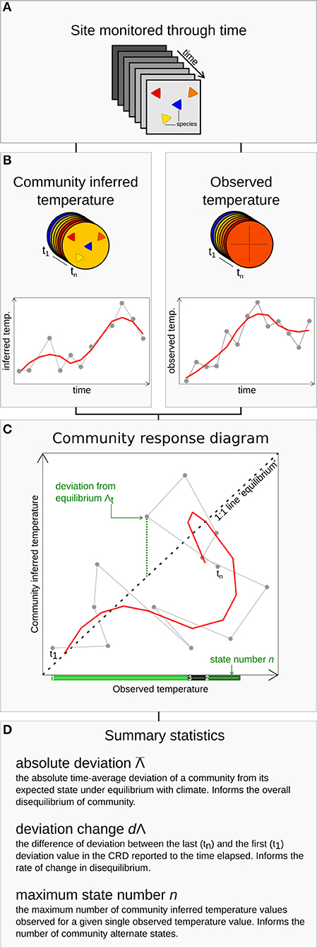
Figure 1. Summary of the community response diagram (CRD) framework. Data on community composition of a given site through time (A) are used to estimate the community-inferred temperature through time (B). Climatic data are used to extract observed temperature of the site through time (C), and the community-inferred temperature through time. These time series are combined in a time-implicit parametric plot to build the CRD (D). For each time bin, deviation from the 1:1 line value and the number of community-inferred value existing for each observed temperature value are used to compute three statistics (E) summarizing different aspects of predictability.

Box 1. Response scenarios between species communities and climatic conditions expected from theory, compiled from Blonder et al. (2017).

1. No-lag scenario

The climate preferences of species in a given community closely match the observed climate. Changes in climate causes an immediate change in community composition so that the climate preference of the present species matches the new climatic conditions.

Expected statistic values : $\bar{\Lambda }$→ 0; dΛ → 0; n = 1

2. Constant-relationship

The community response to climate change has a one-to-one mapping such that the assemblage of species has a unique climatic preference for any observed climate value.

Expected statistic values : $\bar{\Lambda }$ > 0; dΛ → −∞; n = 1

3. Constant-lag

The climate preference of a community follows the observed climate with a fixed time delay. When the response to climate change is linear, this scenario reduce to the constant-relationship scenario. In other cases, the lag could follow a periodic function or the future response of the system might depend on its past history, e.g., via memory effects (hysteresis).

Expected statistic values : $\bar{\Lambda }$ > 0; dΛ → 0; n = 1

4. Alternate unstable states

A generalization of the constant-lag scenario in which the community shows memory effects and the future response to climate depends on the past state of the system. In this scenario, community dynamics follow the observed climate with a variable delay and magnitude. Under such conditions several species assemblages with similar climate preference combinations could occur together with a single value of observed climate. Thus, the future dynamics of the community cannot be predicted only by knowing the current community state.

Expected statistic values : $\bar{\Lambda }$ > 0; dΛ → 0; n = 2

5. Stochastic or chaotic dynamics

Community dynamics are uncorrelated with the observed climate, for example due to stochastic dynamics. As a consequence, many species assemblages with different climate preferences might occur at a given observed climate value.

Expected statistic values : $\bar{\Lambda }$ > 0; dΛ → 0; n > 1

We applied the CRD framework to species community data in two contrasting settings, (i) the long-term dynamics of plant communities during the Late Quaternary climate warming (21 Ka–present) and (ii) the contemporary responses of bird communities to recent temperature changes (1971–2012 C.E.) (Figure S1). We hypothesized that the short-term responses of bird communities to Anthropocene climate change would exhibit a lower predictability than the long-term thermal reshuffling of plant communities during the late Quaternary, for three reasons.

First, short-term variation might be harder to predict than long-term changes because stochasticity is most predominant at fine spatial and temporal scales (Levin, 1992). Second, short-term resistance to unfavorable conditions (Fordham et al., 2016), delayed effect of climate change via indirect effects (e.g., by changing habitats or resource availability, Gaget et al., 2018) and the time needed for species to track climate changes (Alexander et al., 2018) are all expected to increase mismatch in community responses to climate change. In contrast, changes in average temperatures across longer time periods are expected to be balanced with the regional species pools, due to an extended period in which climate induced extinction and colonization could occur (Webb, 1986; Holm and Svenning, 2014). Third, birds might exhibit lower predictability because they are less sensitive to climate change than plants. They have broader thermal tolerances (Araújo et al., 2013), and the relevance of dynamic equilibrium responses as a conceptual model to explain birds responses to climate change is controversial. For example, their realized niche may not necessarily match the observed climate (Beale et al., 2008). Evidence of breeding bird responses to recent climate change are mixed and appear highly idiosyncratic (Stephens et al., 2016; Currie and Venne, 2017).

We also hypothesized that different aspects of community predictability will be structured by environmental and ecological factors, yielding the following predictions:

• More extreme temperature (warm or cold) are linked to stronger disequilibrium in community responses to climate change, with low $\bar{\Lambda }$, negative to null dΛ and n = 1. In the coldest (northern) and warmest (southern) areas of North America, regional species pools might not provide climate-adapted species to local communities (Bertrand et al., 2016) and therefore limit their response to temperature change (Blonder et al., 2015)

• Complex topography is linked to higher predictability, with low $\bar{\Lambda }$, negative to null dΛ and n = 1. In mountainous terrain, we expect strong variation of temperature within small distances to lower the perceived velocity of large scale climate change (Loarie et al., 2009) and therefore increase community thermal response (Bertrand et al., 2011; Gaüzère et al., 2017).

• Human impact is linked to lower predictability, with strong $\bar{\Lambda }$, low dΛ and n > 1. Human impact (i.e., direct exploitation, species introduction, and land conversion) influences community dynamics and also the predictability of community responses to climate change (Maxwell et al., 2016; Bowler and Böhning-Gaese, 2017; Gaget et al., 2018).

Beyond these external factors, we expect biological intrinsic factors to influence community predictability. Assuming that the community mean reflects the local species pool, we predict that:

• Species characteristics increasing dispersal ability are linked to higher predictability, with low $\bar{\Lambda }$, negative to null dΛ and n = 1. Communities consisting of species with a high dispersal potential (lower seed mass, migrant species) respond quickly to climate change (Jenni and Kéry, 2003; Svenning and Skov, 2007).

• Species characteristics increasing persistence in unfavorable environments are linked to lower predictability, with strong $\bar{\Lambda }$, c. null dΛ and n > 1. Life history traits such as longevity, adult height or bodymass increase resistance and persistence to unfavorable climate conditions, therefore decrease the predictability of community.

Methods

Data

Community Data

Plant assemblage composition data across the Late Quaternary and Holocene (21 Ka–present) were compiled from the Neotoma paleoecology database (Goring et al., 2015), relying on the fossil pollen data sets used in Maguire et al. (2016). Sites represent high-quality assemblages and were primarily located in eastern North America. We used Blois et al. (2011) selection of sites and revised chronologies. Pollen assemblages obtained from lake sediments can provide a rough proxy for the composition of communities, despite issues on spatial and taxonomical scale integration, species abundance vs. pollen abundance, and detectability of rare taxa (Birks and Seppä, 2004). These issues might influence the quantification of disequilibrium state because rarer taxa with lower dispersal abilities might be undetected. More details on the data processing, spatial and temporal distributions of site are provided in Figure S1. The overall process yielded a presence/absence dataset comprising 425 sites, 103 plant taxa, and 45 time bins (500 yr each) spanning 21 Ka–present.

Bird assemblage composition across the last 50 years were compiled from the North American Breeding Bird Survey (BBS, Sauer et al., 2013, data and protocol at http://www.pwrc.usgs.gov/bbs/). We used data processed from Barnagaud et al. (2017): first-year observer effects were removed by excluding the first survey performed by a given observer on a given route. The dataset was restricted to 807 routes monitored at least 8 years and once every 5 years during the 1970–2011 period. Coastal, pelagic and species which accounted together for < 1% of the records were not taken into account (87 species). The overall process yielded an abundance dataset comprising 807 routes for up to 435 birds species over 43 years. More details on the data processing, spatial and temporal distributions of the sites are provided in Figure S1.

Temperature Data

Temperature time series in North-America

Paleoclimate time-series data were obtained from SynTraCE-21, a set of transient simulations runs using the CCSM3 model (Liu et al., 2009), with decadal averages stored from 22 Ka to the present. These simulations are reasonably congruent with site-based climate reconstruction (Harrison et al., 2014). Simulations were statistically downscaled to a 0.5° by 0.5° grid cell following the CRU TS 3.20 dataset, and then for every 500 years from 21 to 0 Ka, average maximum temperature was calculated based on a 200 year window centered on the 500 year time step (Lorenz et al., 2016).

Contemporary temperature time-series data were extracted from the Parameter Regression of Independent Slope Model (PRISM) (Oregon Climate Service, Corvallis, OR, USA) for the continental United States (Daly et al., 2000). Both climate datasets were created using point meteorological station data, digital elevation models, and other spatial data sets to generate interpolated gridded estimates of monthly, yearly and event-based climatic parameters. Maps had a spatial resolution of 2.5 arcmin (~3 km cell size at this latitude), as generated by PRISM (Daly et al., 2000).

Global temperature contemporary distribution

Spatial global temperature data used to estimate climate niches (see below) were extracted from WorldClim (http://worldclim.org/version2) raster at 2.5 min of a degree resolution (Fick and Hijmans, 2017). WorldClim rasters at 2.5 min degree provide the best independent descriptors available at global scale, despite the uncertainty and error associated with the values (Hijmans et al., 2005). We used the 2.5 min degree resolution spatial resolution (this is about 4.5 km at the equator) in order to erase micro-climatic variations and local characteristics of the habitat when inferring species thermal niches.

Climate Niches

We inferred realized plant climate niches for mean maximum temperature for each taxon using independent contemporary occurrence data for each species or genus in the paleo-community dataset from the BIEN3 database. We choose maximum temperature as a unique climatic niche axis because it is a strong predictor of the species' responses to temperature increase (Jiguet et al., 2007; Lorenz et al., 2016; Maguire et al., 2016). Note that maximum temperature was strongly correlated with mean temperature and minimum temperature in both paleo and contemporary temperature data (correlation coefficients ranging from 0.89 to 0.98). BIEN3 contains more than 30,000,000 geo-referenced vascular plant observations (Enquist et al., 2009) from a much broader geographic scope than represented by the pollen dataset. Contemporary occurrence data were filtered to include only New World records that did not come from cultivated areas. Genus-level distributions were pooled for taxa with multiple names (e.g., “Ostrya/Carpinus”). For each taxa, we estimated the niche maximum temperature value as the mean of the average monthly maximum temperature values (°C, extracted from the WorldClim raster) over all sites where the taxa was detected. Such realized-niche estimates can be affected by sampling bias, but have the benefit of being estimable from broad-scale and commonly available presence-only data. To ensure that sampling bias does not affect our estimates, we tested the correlation between species' thermal niches estimated from raw data bounded to the 95% confidence interval (i.e., incorporating the density of sampling) with species' thermal niches sampled from a uniform distribution bounded to the 95% confidence interval of real distribution (i.e., without sampling density). A Pearson's product-moment correlation test showed a strong positive correlation between species thermal niches estimated from the different approaches (correlation coefficient ± CI = 0.9967 ± 0.001, t = 120.32, df = 97, p < 0.0001). We concluded that spatial sampling bias is unlikely to affect thermal niche estimates.

We recognize that realized niches for plants may shift over 10³–10⁴ year timescales (Veloz et al., 2012). To check the correlation between paleo and modern niches estimations, we investigated the relationships between paleo-inferred and contemporary-inferred climate niches (Figure S2) and showed that they were closely related (Pearson's correlation coefficient = 0.96, t = 39.9, df = 94, P < 0.0001).

We inferred American bird species' thermal niches by clipping their global extent of occurrence maps onto temperature layers from WorldClim. We used an independent dataset combining global extent-of-occurrence maps for 9,886 bird species (Bird Life International Handbook of the Birds of the World, 2017). BirdLife's species range maps are produced to provide robust, reliable geographic extents of a species range. They are used to present bird distributions on the BirdLife Datazone, the IUCN Red List website and for assessment of individual species Red List status (Bird Life International Handbook of the Birds of the World, 2017). These data have been compiled from multiple sources, including specimens, distribution atlases, survey reports, published literature, and expert opinion, and currently represent the most comprehensive assessment of global bird species occurrences. BirdLife International and HBW endeavor to maintain clean, accurate, and up-to-date data at all times. However, such vector maps do not contain within-range heterogeneity in species' presence, and errors on range margins might be present, especially on ill-sampled avifaunas (Herkt et al., 2017). For each taxon, we estimated the niche maximum temperature value as the breeding-season (May, June, July) average monthly maximum temperature values (°C, extracted from the WorldClim raster) over the breeding distribution range of taxa.

Community Response Diagrams

We used community-inferred temperatures and observed temperatures to build CRDs for the plant and bird datasets, as shown in Figure 1.

First, we computed community-inferred temperature values using the climate niches previously inferred via the species distribution data. For each site monitored at a given time, the community-inferred temperature corresponds to the average climate niche value of all species present in a community. community-inferred temperature was calculated as the average maximum temperature niche value of all species present in a community. We also computed the standard deviation associated with each community-inferred community value.

For birds, we additionally calculated community-inferred temperature based on the abundance-weighted mean of specie's maximum temperature values. This method takes into account the relative abundance of each species in the community and could provide a more sensitive estimation on community-inferred temperature change. Abundance weighted community-inferred temperatures were strongly correlated to estimates based on occurrence only (see Figure S3, Pearson's correlation coefficient = 0.95, t = 540.94, df = 32264, P < 0.0001). We therefore used occurrence-based community-inferred temperature in order to increase the comparability of results between plants and birds.

We then extracted observed maximum temperature for each site and each time bin from paleoclimate and modern time-series data (see Data subsection). In order to reduce the inter-annual variability and temporal stochasticity that might undermine the identification of community and climate dynamics, we smoothed community-inferred and observed temperature times series by using Local Polynomial Regression Fitting (LOESS). LOESS was performed for each time series independently using the loess {stats} R function with an α span of 0.75.

Finally, we built CRDs for each site by sequentially plotting raw and smoothed time series of observed and community-inferred climate values, as shown in Figure 1D. We used CRDs to estimate three complementary statistics depicting predictability of community responses to climate change. For each CRD, the absolute deviation, $\bar{\Lambda }$, was calculated as the absolute value of the average deviation, where the deviation is calculated, for each time value, as the difference between the smoothed value of community-inferred temperature and the smoothed value of observed temperature (Figure 1D). The deviation change, dΛ, was calculated as the difference of deviation between the last and the first time bin of the CRD, divided by the overall timespan of the CRD. The state number, n, was calculated as the number of smoothed community-inferred temperature values (y-axis in CRD) that correspond to a given single value of observed temperature (x-axis in CRD). n counts the number of times a vertical line on the diagram crosses the community-inferred temperature trajectory. Temporal stochasticity and sampling error tend to inflate the state number n through the detection of more than one community state which are statistically not different. To correct for this false detection of n > 1, we tested for the difference between community-inferred temperature values by comparing the difference between 95% confidence interval associated to each community-inferred value. If the 95% confidence interval were overlapping, we inferred that the community-inferred temperature values could not be differentiated, and reduced n by 1 (further called corrected n). More details, formalization, and simulations of CRDs are provided in Blonder et al. (2017). R scripts and functions used to compute these summary statistics and other descriptive metrics can be found at https://github.com/pgauzere/Predictability_CRD.

Predictors

For both plants and birds, we gathered a set of five explanatory variables associated to community responses to changes in temperature: two abiotic variables (i.e., baseline temperature and topography), one variable related to human influence on ecosystems (i.e., paleo human density for plants, contemporary human influence index for birds), and two variables related to species characteristics known to influence tracking and resistance processes (i.e., seed mass and plant height for plants, body mass, and migration for birds). The distributions and mapping of predictors variables are shown in Figure S4. Note that none of our pairs of predictors were strongly correlated (maximum correlation coefficient was 0.41 for baseline climate-topography).

Baseline Temperature

To test for the effect of climate on community predictability, we extracted the baseline maximum temperature of each site as the first observed maximum temperature value recorded for a given site. See Temperature Data section.

Topography

To estimate topography, we extracted digital elevation data (DEMs) from the NASA Shuttle Radar Topographic Mission (SRTM). The NASA SRTM provides elevation as 3 arc second (~90 m) resolution. For each site, we calculated a topography index as the difference between highest and lowest elevation within a 50 km buffer around the site. We tested the influence of the buffer size on our estimate by computing topography on 100 and 150 km buffer and comparing these values to the 50 km buffer.

Human Imprint on Ecosystems

To estimate the human imprint on ecosystems over the Holocene period, we obtained population density data over the Holocene for the period ranging from 21 to 0 Ka from the HYDE 3.2 database (Klein Goldewijk et al., 2011). These data are chosen to provide an approximate proxy for the upper bound of human impacts on communities across the last 21 Ka. We extracted population density value for each site from Neotoma dataset. To estimate the contemporary human imprint on ecosystems, we used the Global Human Influence Index (HII) from the NASA Socioeconomic Data and Applications Center. This index estimates the direct human footprint on ecosystems (Sanderson et al., 2002) as a proxy of recent human pressure on biodiversity. HII incorporates nine global data layers corresponding to population density, human land use, infrastructure, and human access. We extracted HII values for each site from BBS dataset using the raster library.

Species Characteristics

For plants, we computed the community mean seed mass and plant height (Honnay et al., 2002; Matlack, 2005; Normand et al., 2011) using traits values compiled from the TRY database (Kattge et al., 2011). For birds, we used mean body mass and the percent of migrants of each community (Jiguet et al., 2007; Angert et al., 2011) using traits from the Encyclopedia Of Life (http://www.eol.org), the Animal Diversity Web (http://www.animaldiversity.org) and the field guide to North American birds (Sibley, 2014) previously compiled in Barnagaud et al. (2017).

Statistical Analysis

We tested the effect of our set of predictors on each CRD summary statistic by implementing generalized additive models (GAM). We ran six models in which each statistic was the response variable ($\bar{\Lambda }$, dΛ, and n. for both plants and birds) regressed over a set of five predictors (for plants: baseline climate, topography, human density, mean seed mass, means plant height; for birds: baseline climate, topography, human influence index, mean body mass, percent of migrant species). We estimated the linear effect of each predictor, and added a two-dimensional spline based on geographic coordinates in order to account for spatial autocorrelation (Wood, 2006). Because we predicted the effect of baseline climate to occur at coldest and warmest conditions, our models included both linear and quadratic terms for baseline climate. Because state number (n) values take positive integer values, we used Poisson GAMs to analyze these data. Strong outliers corresponding to site with very low number of taxa, or strong variations of number of taxa through time were deleted for the analysis (between one and five points depending on models). P-values reported for parametric and smoothed model terms were based on Wald tests. All analyses were performed using the mgcv library in R statistical software (R Development Core Team, 2013). The code written for data analysis can be accessed at https://github.com/pgauzere/Predictability_CRD.

Results

We found strong support for disequilibrium dynamics in both plant and bird responses to climate change. We described a wide variation in the type of community dynamics, with CRD depicting potential evidence for all scenarios listed in Box 1. CRD for a few representative communities are shown in Figure 2. All CRDs, along with associated time series and statistics values are shown in Figure S5.

FIGURE 2

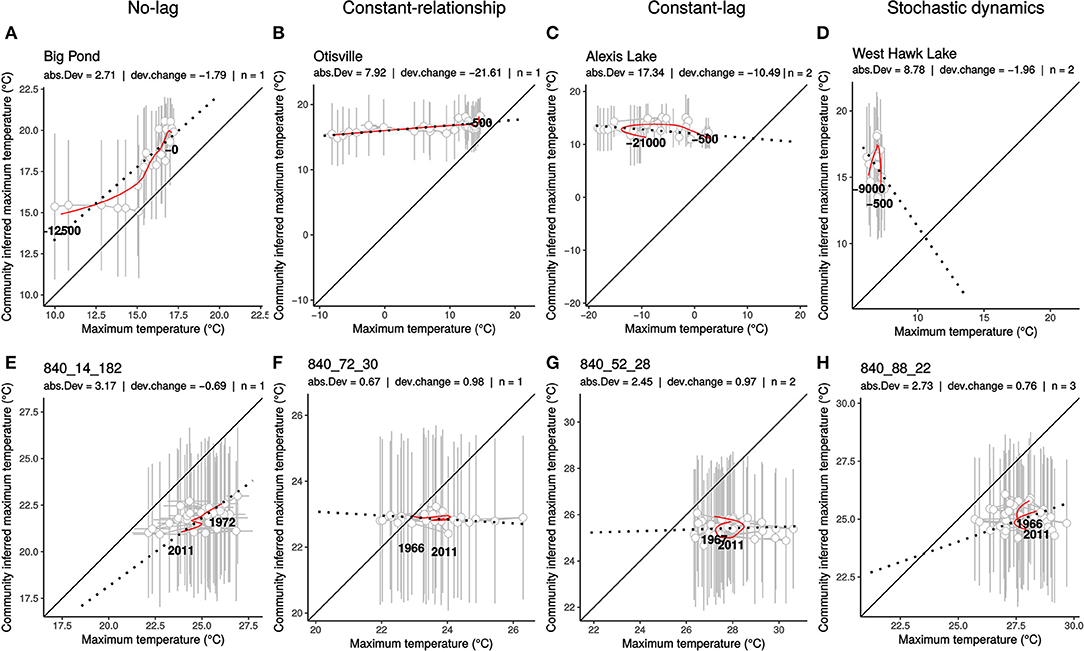
Figure 2. Examples of representative community response diagrams (CRD). Representative CRD from plant community responses during Late Quaternary climate change (top, A–D) and birds community responses between 1966 and 2011 (C,E) (bottom, E–H). For each CRD, community-inferred maximum temperature (y-axis) is plotted over observed maximum temperature in a time-implicit diagram. Gray points and bars are raw mean values with associated standard deviations. Red lines are smoothed values used to compute statistics. Black lines are 1:1 relationship, dotted black lines represent the linear regression of the smoothed values. Name of the site and summary statistics are reported at the top of each panel, abs.Dev = absolute deviation $\bar{\Lambda }$, dev.change = deviation change dΛ, n = maximum state number n.

The main component explaining the three summary statistics from the CRD was baseline climate. In the multivariate models, baseline climate was consistently related to variations of CRD statistics (baseline climate has a significant effect on statistics in five over six GAMs performed, Figure 2). Apart from baseline climate, no clear general pattern emerged from other predictors. The geographic two-dimensional splines smooth terms included in the model substantially increased the fit of the models for the absolute deviation and the deviation change but did not increase the fit of the model for maximum state number. Overall, our set of predictors explained from 20.9 to 80.5% of the deviance (apart from n for birds).

Plants

Scenarios of Responses

Plant communities generally exhibited lagged monotonic and positive relationship between inferred and observed temperatures during the last 21 Ka. A few communities (2.4%) showed no-lag (or low-lag) dynamics, where relationships between inferred community and observed temperature are linear and close to the 1:1 line. These communities were characterized by $\bar{\Lambda }$ < 5°C, −2 < dΛ < 2°C.Ka⁻¹, and n = 1 (Figure 2A). Many communities (60.0%) showed approximately constant-relationship dynamics, where increases in temperature lead to monotonic and non-linear change in community-inferred temperature. These communities were characterized by $\bar{\Lambda }$>5°C, dΛ < 0°C.Ka⁻¹ and n = 1 (Figure 2B). In plant communities, a particular constant-relationship dynamic was commonly observed. It was characterized by communities having strong baseline deviation from climatic equilibrium that did not exhibit substantial variation in community-inferred temperature while observed temperature strongly increased. Such dynamics led to a strong decrease in deviation through time (Figure 2B). Some communities (23.0%) showed approximately constant-lag dynamics with partial or complete loops (Figure 2C) or stochastic dynamics (Figure 2D). These communities were characterized by −2 < dΛ < 2°C.Ka⁻¹ and n >1 (Figure 2C).

Summary Statistics

Generally, plant communities did show a large deviation between observed and inferred climate ($\bar{\Lambda }$ = 8.37 ± 3.4 °C [mean ± sd], Figure 3) and did not follow a 1:1 equilibrium state with climate. $\bar{\Lambda }$ values were structured in space, with high values of $\bar{\Lambda }$ at northern and southern latitudes and lower $\bar{\Lambda }$(< 5°C, see Figure 3) at mid latitudes. Across the study sites this deviance from equilibrium was constant through the last 21 Ka (dΛ = −0.54 ± 0.63 °C.Ka⁻¹). However, ~85% of the communities did show negative dΛ values (suggesting that the amount of climate disequilibrium did decrease at these sites). Low dΛ values did peak at mid latitudes (Figure 3). The maximum state number n ranged from 1 to 4. 24.5% of the sites had more than one state number for a specific observed temperature temperature during the time series. Thus, in a quarter of the communities the inferred temperature value can have multiple values for a single observed temperature. Maximum state number n tended to peak in boreal latitudes.

FIGURE 3

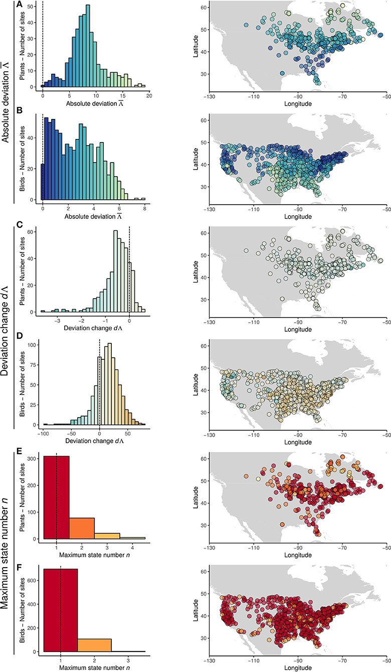
Figure 3. Distributions (left panels) and maps (right panels) of summary statistics (A,B: absolute deviation $\bar{\Lambda }$; C,D: deviation change dΛ; E,F: maximum state number, n) estimated from CRD for plants (A,C,E) and birds (B,D,F). Colors correspond to the statistics value, as shown in distributions. Broken black lines represent expectation from no-lag scenario.

Factors Structuring Equilibrium Dynamics

Absolute deviation $\bar{\Lambda }$ decreased with increasing baseline temperature (Baseline.Climate coefficient = −1.34 ± 0.089 [mean ± Standard Error], z = −15.02, ***P < 0.001, Figure 4A left panel), with saturation on warmest conditions (Baseline Climate² coefficient = 0.49 ± 0.09, z = 5.71, ***P < 0.001, Figure 4A left panel). $\bar{\Lambda }$ also decreased with increasing mean plant height (Plant height coefficient = −0.32 ± 0.10, z = −3.02, **P < 0.001, Figure 4A left panel). The geographic splines smooth terms were significantly improving the fit of the model (edf = 33.8, F = 21.82, ***P < 0.001). The full model (i.e., including a 2-dimensional spline based on geographic coordinates) explained 92.8% of the deviance, excluding the geographical spline reduced the explained deviance to 70.2%. Thus, deviation from equilibrium state was generally higher for plant communities situated in coldest areas and composed of shortest plant species.

FIGURE 4

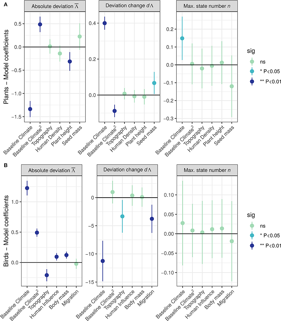
Figure 4. Effect of predictors on plant (A) and bird (B) summary statistics (absolute deviation $\bar{\Lambda }$, left panel; deviation change dΛ, middle panel, maximum state number n, right panel), estimated as linear coefficients (± 95% confidence intervals) from generalized additive mixed models. Topography and Human Density were square-root transformed. All predictors were scaled to mean = 0 and SD = 1 prior to modeling to ease comparisons. Point and bar colors indicate the significance level associated to the test (light green: non-significant; light blue: significant at α = 5%; dark blue: significant at α = 1%).

Deviation change dΛ increased with baseline temperature (Baseline.Climate coefficient = 0.34 ± 0.019 SE, z = 21.45, **P < 0.001, Figure 4A mid panel), with saturation on warmest conditions (Baseline.Climate² coefficient = −0.09 ± 0.09 SE, z = 4.97, ***P < 0.001, Figure 4A mid panel). dΛ also slightly increased with increasing mean seed mass (Seed.mass coefficient = 0.07± 0.03 SE, z = 2.13, *P < 0.05, Figure 4A mid panel). The geographic splines smooth terms were significantly improving the fit of the model (edf = 26.32, F = 6.94, ***P < 0.001). The full model explained 84.1% of the deviance (51.3% without geographical spline). Thus, deviation from equilibrium state increase through time for plant communities situated in warmer areas.

Maximum state number n increased with increasing baseline temperature (Baseline.Climate coefficient = 0.14 ± 0.06, z = 2.39, *P < 0.05, Figure 4A right panel). The geographic splines smooth terms did not improve the fit of the model (edf = 3.59, Chi.sq = 5.076, P = 0.17). The full model explained 34.4% of the deviance (20.9% without geographic splines).

Birds

Scenarios of Responses

Bird communities generally exhibited non-directional and stochastic dynamics in climate responses between 1966 and 2011. A few communities (1.4%) showed no-mismatch or low-mismatch dynamics, where relationships between inferred community and observed temperature are linear and close to the 1:1 line. These communities were characterized by $\bar{\Lambda }$ < 2°C, −20 < dΛ < 20°C.Ka⁻¹, and n = 1 (Figure 2E). A few communities (3.4%) showed approximately constant-relationship dynamics, where increases in temperature lead to monotonic and non-linear change in community-inferred temperature. These communities were characterized by $\bar{\Lambda }$>2°C, dΛ < −20°C.Ka⁻¹ and n = 1 (Figure 2F). A few communities (2%) showed approximately constant-lag or stochastic dynamics with partial or complete loops. These communities were characterized by −20 < dΛ < 20°C.Ka⁻¹, and n >1 (Figure 2G). However, many bird communities (c. 60%) exhibited non-directional and stochastic dynamics of response to observed temperatures (strong absolute deviation and low deviation change) with n = 1 (Figure 2H). Such stochastic dynamics associated with low state number are mainly due to the correction applied to the estimation of n, and are hard to identify (see Figure S4).

Summary Statistics

Bird communities showed a consistent deviation from climate equilibrium ($\bar{\Lambda }$ = 2.41 ± 1.86°C, Figure 3). $\bar{\Lambda }$ was structured in space, with higher values of $\bar{\Lambda }$ in the south-eastern part of North America. On average, equilibrium states did not change in the bird communities between 1966 and 2011 (dΛ = 10.06 ± 19.64°C.Ka⁻¹). However, 73.2% of the sites did show positive dΛ values (e.g., an increase in climatic disequilibrium). The lowest negative values of dΛ were present in Western North America, while positive values were generally distributed in south-eastern North America.

Ninety-eight percent of the sites had a maximum state number n = 1, indicating that predictability is reachable for a large part of the communities. However, over this interval there was limited directional change in climate (see CRD), which would also be consistent with slow but stochastic dynamics. The low n value was mainly due to the correction we applied to take into account the strong stochasticity associated with these dynamics (see sections Methods-Community Response Diagrams and Discussion). On average, the uncorrected n value was strong (mean ± sd = 3.2 ± 0.76), with 99% of sites having n > 1 and 88% of sites having n > 2. The max state number n did not exhibit any spatial pattern.

Factors Structuring Equilibrium Dynamics

Absolute deviation $\bar{\Lambda }$ increased with increasing baseline temperature (Baseline.Climate coefficient = 1.17 ± 0.054 SE, z = 21.51, P < 0.001**, Figure 4B, left panel), with saturation on coldest conditions (Baseline.Climate² coefficient = 0.54 ± 0.0304, z = 14.19, P < 0.001***, Figure 4B, left panel). $\bar{\Lambda }$ increased with decreasing topography (Topography coefficient = −0.16 ± 0.045, z = −3.72, ***P < 0.001) and increasing mean body mass (Body mass coefficient = 0.106 ± 0.0275 SE, z = 4.12, ***P < 0.001). The geographic splines smooth terms were significantly improving the fit of the model (edf = 45.26, F = 26.79, ***P < 0.001). The full model explained 93.4% of the deviance (81.6% without geographical spline). Overall, deviation from equilibrium state was generally higher for bird communities situated in warmer and mountainous areas with high human influence and those composed of larger species.

Deviation change dΛ decreased with increasing baseline temperature (Baseline.Climate coefficient = −8.45 ± 1.62, z = −6.13, ***P < 0.001, Figure 4A, mid panel). Furthermore, dΛ slightly decreased (effect significant at α = 10%) with increasing topography (Topography coefficient = −2.33 ± 1.31, z = −1.77, P = 0.076 ns). The geographic splines smooth terms were significantly improving the fit of the model (edf = 40.97, F = 5.84, ***P < 0.001). The full model explained 44.5% of the deviance (17.7% without geographical spline). Deviation from equilibrium state decreased through time for bird communities situated in warmer, mountainous areas, and composed of higher proportion of migratory birds.

Maximum state number n was not related with any of our predictors (Figure 4B, right panel). The geographic splines smooth terms were not improving the fit of the model (edf = 0, Chi.sq = 0, P = 1). The full model explained 2.3% of the deviance (1% without geographical spline).

Discussion

We explored the limits and the determinants of predictability in community responses to climate change in bird and plant assemblages using CRDs. Currently, anticipatory prediction of biodiversity responses to climate change have considered a limited range of dynamics, relying on predictable relationships between species or community dynamics and climate change. While the no-lag equilibrium hypothesis is the implicit foundation of species distribution modeling (Peterson et al., 2011), only recent extensions of this method has successfully considered constant lag or constant relationship by incorporating dispersal limitation and/or properties of species assemblages (Guisan and Rahbek, 2011; Zurell et al., 2016). We here provided potential evidence for all types of community dynamics (see Box 1), including unpredictable dynamics (e.g., alternate states and stochastic dynamics) which are often not considered in current modeling approaches. Our work suggests that the current understanding of community dynamics in relation to climate change is oversimplified. Among the responses described in our study, equilibrium dynamics were the exception rather than the norm. This result challenges the equilibrium dynamic as the fundamental concept for predictive models of biodiversity response to climate change.

Along with the equilibrium dynamics hypothesis, the space-for-time substitution approach has often been used to predict the effects of climate change on biodiversity. Although this assumed equivalence may be relevant in situations where equilibrium dynamics prevails (Walker et al., 2010), many studies have emphasized substantial differences between spatial and temporal responses (Johnson and Miyanishi, 2008). Our work suggests that because many community dynamics are diverging from equilibrium, the space-for-time substitution approach should be used with caution to infer future community state. Temporal dynamics might provide fundamentally different insights than spatial patterns (Bonthoux et al., 2013; Bjorkman et al., 2018). While ecology is undergoing a major transformation to leverage and synthesize more spatial datasets (Hampton et al., 2013), time-series data and analysis are more than ever needed to reach a better understanding and predictability of non-equilibrium biodiversity responses to climate change.

For plants, the most common type of dynamics reported were constant-relationship scenarios. Such dynamics were impaired with strong lagged responses. The current distribution of North American plants are heavily affected by climatic conditions at the Last Glacial Maximum (Ordonez, 2013), and plants are known to show dispersal lags in post-glaciated areas (Normand et al., 2011). This explains the persistence of deviation in responses between observed and inferred climate in North American plant communities across the last 21 Ka. Constant-relationship scenarios responses might be predictable by modeling approaches considering dispersal and community assembly rules (Guisan and Rahbek, 2011). However, almost a quarter of the plant communities exhibited unpredictable dynamics such as constant-lag and alternate stable states.

Bird communities mainly exhibited unpredictable dynamics. Community dynamics appeared stochastic, and often uncorrelated with the observed climate. Despite the fact that maximum temperature change was generally not strong or directional (see Figure S5), the complex disequilibrium observed in bird communities compared to the plant communities is in line with our expectations. Two reasons can explain the stochasticity observed in bird responses to modern climate change. Firstly, climatic determinism of northern hemisphere bird communities is questionable (Beale et al., 2008; Currie and Venne, 2017). For example, broad thermal tolerances (Araújo et al., 2013) and phenological responses (Stenseth et al., 2002; Dunn and Winkler, 2010) might buffer the impact of moderate temperature changes on communities dynamics (Gaüzère et al., 2015). Moreover, bird sensitivity to habitat changes probably influences community-inferred temperatures (Clavero et al., 2011; Barnagaud et al., 2013) and overrides the direct effect of climate warming on community dynamics (Eglington and Pearce-Higgins, 2012; Gaget et al., 2018).

Secondly, short-term variation might be harder to predict than long-term changes because stochastic variability is predominant at fine spatial and temporal scales (Levin, 1992). However, consistent short-term directional changes in bird community-inferred temperature have been reported at continental (Devictor et al., 2012; Princé and Zuckerberg, 2015), national (Devictor et al., 2008), and landscape scales (Gaüzère et al., 2015). Our results showed that local-scale changes in community-inferred temperature were not consistently related to observed temperature change. The scale of effect is defined as the scale at which an environmental attribute has the strongest effect on inferred species-environment relationship. While it is known as a strong determinant of explanatory predictions (Holland et al., 2004; de Knegt et al., 2010), many empirical studies might not be conducted at the appropriate spatial scales (Jackson and Fahrig, 2015). Hence, we can hypothesize that the low predictability exhibited by breeding bird communities might be due to the weak climatic determinism of bird community dynamics at local scale. This suggest that using equilibrium dynamics hypothesis as a conceptual model to predict biodiversity responses to climate change requires caution. We argue that a careful assessment of climate determinism focused on the taxon and the scale of study is a prerequisite for successful anticipatory predictions.

We also showed that some aspects of predictability—absolute deviation from climate equilibrium and deviation change—were structured by environmental or ecological factors, while others—number of alternate states—were not. We expected community predictability to decrease with thermal severity. Our results showed that absolute deviation of plant communities was decreasing with temperature, with a curvilinear relationship showing a plateau on warmest values. Conversely, absolute deviation for birds was increasing with increasing temperature before reaching a plateau. This apparent discrepancy between plants and birds is linked to the distribution of Neotoma and BBS sites. Neotoma sites are distributed in northwestern Nearctic margin and are therefore colder than BBS sites distributed in southern Nearctic margin. Merging the BBS and Neotoma estimates showed a quadratic relationship between absolute deviation and baseline temperature (Figure S6). As expected, overall absolute deviation increased with coldest and warmest temperature. The consistent effect of baseline climate between taxa and spatial scale suggest a strong regional-scale determinism of predictability, structured by the diversity of realized thermal niches in the regional species pool. In France, Bertrand et al. (2016) already reported a strong effect of baseline temperature on deviation from equilibrium state, in link with the absence of climate-adapted species in the regional pool. Climate severity is expected to have an even stronger effect in North America. The distribution of land masses constrains Neartic species' distribution range in their northern and southern boundaries. These geometric constraints on species distribution, also called “mid-domain effect,” are known to shape latitudinal richness gradient (Colwell and Lees, 2000). While its application to non-spatial domains is scarce (but see Letten et al., 2013), the “thermal mid-domain effect” probably have a strong influence on the species' thermal tolerance present in regional species pools (Brayard et al., 2005; Beaugrand et al., 2013). This suggest that long-term biogeographic history and macro-scale processes have a strong influence on community predictability. Further investigations of the thermal mid-domain effect and its consequence on regional pools should clarify its implication in the predictability of community responses to climate change.

Our analysis showed that plant communities composed of taller plants exhibited lower absolute deviation from climate equilibrium. This result is in line with our predictions. No-lag dynamics and predictable responses are thought to occur when species exhibit low persistence through rapid extinction at trailing range edges (Hampe and Petit, 2005), and/or efficient niche tracking through long-distance dispersal. Conversely, disequilibrium responses are thought to occur when species' responses in these domains are opposite (Svenning and Sandel, 2013). In turn, the importance of these processes is linked to species' dispersal ability and life-history traits. For example, species traits related to weak dispersal ability decrease species' niche tracking (Svenning and Skov, 2007) while persistence processes are enhanced by survival of long-lived individuals (Eriksson, 1996; Holt, 2009; Jackson and Sax, 2010). However, we did not find support for the effect of seed mass on the predictability. While lower seed mass is generally considered as a proxy for longer dispersal distance, empirical evidence is mixed (Thomson et al., 2011). Plant height might even be better predictor for seed dispersal distance (Muller-Landau et al., 2008; Thomson et al., 2011). Because dispersal limitation is expected to be a major driver of climate disequilibrium for plants (Svenning and Skov, 2007, but see Bertrand et al., 2016), the improved dispersal of taller plants supported our result.

For birds we showed that, as predicted, communities composed of larger birds exhibited stronger absolute deviation. Despite the fact that body mass is an integrative species characteristic correlated with many life-history traits, this result confirms that life history traits can influence birds responses through niche tracking and persistence processes (Jiguet et al., 2007). Note that side analyses incorporated the percent of insectivorous birds species as a potential determinant of predictability (Figure S7). This predictor was removed from our final model to keep consistency between plant and bird analyses.

Nevertheless, the influence of species characteristics was generally weak, and not consistent across taxa and CRD statistics. While trait might be good predictors for population responses to climate change (e.g., Julliard et al., 2003; Jiguet et al., 2007), there is weak support for their effect on species' distribution range shifts (Angert et al., 2011; Tingley et al., 2012; Smith et al., 2013). Different reasons such as the stochastic nature of colonization events, novel species interactions and extrinsic effects of habitat availability and fragmentation might explain these weak effects. Moreover, the properties of species assemblages and assembly rules might be more important for community scale dynamics (Guisan and Rahbek, 2011).

Our set of predictors failed to explain variation in maximum state number. This statistic is a key component of predictability. However, accounting for sampling error challenges a straightforward interpretation of n-values when applied to stochastic dynamics. Without sampling error, stochastic dynamics are expected to cause high n values associated with low predictability. For birds, the uncorrected n values were, indeed, high (99% of the sites having n > 1 and 88% of the sites having n > 2), but the necessary correction starkly reduced this estimate (14% of the sites having n > 1 after correcting for sampling uncertainty).

Conclusion

A better understanding of the limits to predictability is a crucial step for predictive modeling and applied ecology (Mouquet et al., 2015). Our study showed that the equilibrium dynamic hypothesis to infer community responses to climate change is only sometimes applicable. In many cases, a straightforward application of the equilibrium dynamic hypothesis to predict biodiversity responses to future climate changes may lead to misleading predictions. Equilibrium dynamics across different taxa and scales should be assumed cautiously. We argue that robust anticipatory predictions will require detailed knowledge of the taxa considered, along with the spatial and temporal scales at which key processes are expected to drive biodiversity response to climate change.

Author Contributions

PG and BB designed the study and performed the analysis. PG wrote the first draft of the manuscript. All authors contributed substantially to the conceptual aspect of the study, and to the writing and revisions of the manuscript.

Conflict of Interest Statement

The authors declare that the research was conducted in the absence of any commercial or financial relationships that could be construed as a potential conflict of interest.

Acknowledgments

We sincerely and warmly thank the NEOTOMA database group and the thousands of dedicated volunteers who took part in the North American Breeding Bird Survey (BBS) to collect the valuable data used in our analysis. We also thanks Jessica Blois for providing the paleo datasets, Carolyn Flower for kindly editing the English, all the Macrosystems Ecology Lab (http://benjaminblonder.org/research/) for their insights on the project, and reviewers and editor Giovanni Rapacciuolo for their valuable comments. J-CS considers this work a contribution to his VILLUM Investigator project Biodiversity Dynamics in a Changing World funded by VILLUM FONDEN (grant 16549). LI was supported by the Carlsberg Foundation (grant CF17-0155).

Supplementary Material

The Supplementary Material for this article can be found online at: https://www.frontiersin.org/articles/10.3389/fevo.2018.00186/full#supplementary-material

References

Alexander, J. M., Chalmandrier, L., Lenoir, J., Burgess, T. I., Essl, F., Haider, S., et al. (2018). Lags in the response of mountain plant communities to climate change. Glob. Chang. Biol. 24, 563–579. doi: 10.1111/gcb.13976

PubMed Abstract | CrossRef Full Text | Google Scholar

Angert, A. L., Crozier, L. G., Rissler, L. J., Gilman, S. E., Tewksbury, J. J., and Chunco, A. J. (2011). Do species' traits predict recent shifts at expanding range edges? Ecol. Lett. 14, 677–689. doi: 10.1111/j.1461-0248.2011.01620.x

PubMed Abstract | CrossRef Full Text | Google Scholar

Araújo, M. B., Ferri-Yáñez, F., Bozinovic, F., Marquet, P. A., Valladares, F., and Chown, S. L. (2013). Heat freezes niche evolution. Ecol. Lett. 16, 1206–1219. doi: 10.1111/ele.12155

PubMed Abstract | CrossRef Full Text | Google Scholar

Ash, J. D., Givnish, T. J., and Waller, D. M. (2017). Tracking lags in historical plant species' shifts in relation to regional climate change. Glob. Chang. Biol. 23, 1305–1315. doi: 10.1111/gcb.13429

PubMed Abstract | CrossRef Full Text | Google Scholar

Barnagaud, J. Y., Barbaro, L., Hampe, A., Jiguet, F., and Archaux, F. (2013). Species' thermal preferences affect forest bird communities along landscape and local scale habitat gradients. Ecography 36, 1218–1226. doi: 10.1111/j.1600-0587.2012.00227.x

CrossRef Full Text | Google Scholar

Barnagaud, J. Y., Gaüzère, P., Zuckerberg, B., Princé, K., and Svenning, J. C. (2017). Temporal changes in bird functional diversity across the United States. Oecologia 185, 737–748. doi: 10.1007/s00442-017-3967-4

PubMed Abstract | CrossRef Full Text | Google Scholar

Beale, C. M., Lennon, J. J., and Gimona, A. (2008). Opening the climate envelope reveals no macroscale associations with climate in European birds. Proc. Natl. Acad. Sci. U.S.A. 105, 14908–14912. doi: 10.1073/pnas.0803506105

PubMed Abstract | CrossRef Full Text | Google Scholar

Beaugrand, G., Rombouts, I., and Kirby, R. R. (2013). Towards an understanding of the pattern of biodiversity in the oceans. Glob. Ecol. Biogeogr. 22, 440–449. doi: 10.1111/geb.12009

CrossRef Full Text | Google Scholar

Bertrand, R., Lenoir, J., Piedallu, C., Riofrío-Dillon, G., de Ruffray, P., Vidal, C., et al. (2011). Changes in plant community composition lag behind climate warming in lowland forests. Nature 479, 9–12. doi: 10.1038/nature10548

PubMed Abstract | CrossRef Full Text | Google Scholar

Bertrand, R., Riofrío-Dillon, G., Lenoir, J., Drapier, J., de Ruffray, P., Gégout, J. C., et al. (2016). Ecological constraints increase the climatic debt in forests. Nat. Commun. 7:12643. doi: 10.1038/ncomms12643

PubMed Abstract | CrossRef Full Text | Google Scholar

Bird Life International Handbook of the Birds of the World (2017). Bird Species Distribution Maps of the World. Bird species Distrib. maps world Version 2017.2. Available online at: http://datazone.birdlife.org/species/requestdis

Birks, H. H., and Ammann, B. (2000). Two terrestrial records of rapid climatic change during the glacial-Holocene transition (14,000- 9,000 calendar years B.P.) from Europe. Proc. Natl. Acad. Sci. U.S.A. 97, 1390–1394. doi: 10.1073/pnas.97.4.1390

PubMed Abstract | CrossRef Full Text | Google Scholar

Birks, H. J. B., and Seppä, H. (2004). Pollen-based reconstructions of late-Quaternary climate in Europe - Progress, problems, and pitfalls. Acta Palaeobot. 44, 317–334.

Google Scholar

Bjorkman, A. D., Myers-Smith, I., Elmendorf, S., Normand, S., Rüger, N., Beck, P. S. A., et al. (2018). Change in plant functional traits across a warming tundra biome. Nature 562, 57–62. doi: 10.1038/s41586-018-0563-7

CrossRef Full Text | Google Scholar

Blois, J. L., Williams, J. W. J., Grimm, E. C., Jackson, S. T., and Graham, R. W. (2011). A methodological framework for assessing and reducing temporal uncertainty in paleovegetation mapping from late-Quaternary pollen records. Quat. Sci. Rev. 30, 1926–1939. doi: 10.1016/j.quascirev.2011.04.017

CrossRef Full Text | Google Scholar

Blois, J. L. J. L., Williams, J. W. J. W., Fitzpatrick, M. C. M. C., Jackson, S. T., and Ferrier, S. (2013). Space can substitute for time in predicting climate-change effects on biodiversity. Proc. Natl. Acad. Sci. U.S.A. 110, 9374–9379. doi: 10.1073/pnas.1220228110

PubMed Abstract | CrossRef Full Text | Google Scholar

Blonder, B., Enquist, B. J., Graae, B. J., Kattge, J., Maitner, B. S., Morueta-Holme, N., et al. (2018). Late Quaternary climate legacies in contemporary plant functional composition. Glob. Chang. Biol. 24, 4827–4840. doi: 10.1111/gcb.14375

PubMed Abstract | CrossRef Full Text | Google Scholar

Blonder, B., Moulton, D. E., Blois, J., Enquist, B. J., Graae, B. J., Macias-Fauria, M., et al. (2017). Predictability in community dynamics. Ecol. Lett. 20, 293–306. doi: 10.1111/ele.12736

PubMed Abstract | CrossRef Full Text | Google Scholar

Blonder, B., Nogués-bravo, D., Borregaard, M. K., John, C., Ii, D., Jørgensen, P. M., et al. (2015). Linking environmental filtering and disequilibrium to biogeography with a community climate framework. Ecology 96, 972–985. doi: 10.1890/14-0589.1

PubMed Abstract | CrossRef Full Text | Google Scholar

Bonthoux, S., Barnagaud, J. Y., Goulard, M., and Balent, G. (2013). Contrasting spatial and temporal responses of bird communities to landscape changes. Oecologia 172, 532–574. doi: 10.1007/s00442-012-2498-2

PubMed Abstract | CrossRef Full Text | Google Scholar

Bowler, D., and Böhning-Gaese, K. (2017). Improving the community-temperature index as a climate change indicator. PLoS ONE 12:e0184275. doi: 10.1371/journal.pone.0184275

PubMed Abstract | CrossRef Full Text | Google Scholar

Brayard, A., Escarguel, G., and Bucher, H. (2005). Latitudinal gradient of taxonomic richness: combined outcome of temperature and geographic mid-domains effects? J. Zool. Syst. Evol. Res. 43, 178–188. doi: 10.1111/j.1439-0469.2005.00311.x

CrossRef Full Text | Google Scholar

Clark, J. S., Carpenter, S. R., Barber, M., Collins, S., Dobson, A., Foley, J. A., et al. (2001). Ecological forecasts: an emerging imperative. Science 293, 657–661. doi: 10.1126/science.293.5530.657

PubMed Abstract | CrossRef Full Text | Google Scholar

Clavero, M., Villero, D., and Brotons, L. (2011). Climate change or land use dynamics: do we know what climate change indicators indicate? PLoS ONE 6:e18581. doi: 10.1371/journal.pone.0018581

PubMed Abstract | CrossRef Full Text | Google Scholar

Colwell, R. K., and Lees, D. C. (2000). The mid-domain effect: geometric constraints on the geography of species richness. Trends Ecol. Evol. 15, 70–76. doi: 10.1016/S0169-5347(99)01767-X

PubMed Abstract | CrossRef Full Text | Google Scholar

Currie, D. J., and Venne, S. (2017). Climate change is not a major driver of shifts in the geographical distributions of North American birds. Glob. Ecol. Biogeogr. 26, 333–346. doi: 10.1111/geb.12538

CrossRef Full Text | Google Scholar

Daly, C., Taylor, G. H., Gibson, W. P., Parzybok, T. W., Johnson, G. L, and Pasteris, P. A (2000). High-quality spatial climate data sets for the united states and beyond. Trans. ASAE 43, 1957–1962. doi: 10.13031/2013.3101

CrossRef Full Text | Google Scholar

De Frenne, P., Rodriguez-Sanchez, F., Coomes, D. A., Baeten, L., Verstraeten, G., Vellend, M., et al. (2013). Microclimate moderates plant responses to macroclimate warming. Proc. Natl. Acad. Sci. U.S.A. 110, 18561–18565. doi: 10.1073/pnas.1311190110

PubMed Abstract | CrossRef Full Text | Google Scholar

de Knegt, H. J., van Langevelde, F., Coughenour, M. B., Skidmore, A. K., de Boer, W. F., Heitkönig, I. M. A., et al. (2010). Spatial autocorrelation and the scaling of species — environment relationships. Ecology 91, 2455–2465. doi: 10.1890/09-1359.1

PubMed Abstract | CrossRef Full Text | Google Scholar

Devictor, V., Julliard, R., Couvet, D., and Jiguet, F. (2008). Birds are tracking climate warming, but not fast enough. Proc. R. Soc. B Biol. Sci. 275, 2743–2748. doi: 10.1098/rspb.2008.0878

CrossRef Full Text | Google Scholar

Devictor, V., van Swaay, C., Brereton, T., Brotons, L., Chamberlain, D., Heliölä, J., et al. (2012). Differences in the climatic debts of birds and butterflies at a continental scale. Nat. Clim. Chang. 2, 121–124. doi: 10.1038/nclimate1347

CrossRef Full Text | Google Scholar

Dunn, P. O. P., and Winkler, D. (2010). “Effects of climate change on timing of breeding and reproductive success in birds,” in Effects of Climate Change on Birds (Oxford University Press), 113–126. Available online at: http://books.google.com/books?hl=en&lr=&id=EhVwombWTpcC&oi=fnd&pg=PA113&dq=Effects+of+climate+change+on+timing+of+breeding+and+reproductive+success+in+birds&ots=NrQRX80JVm&sig=J7Ue8N7lvIJxY2kLbZnEMre_eqM (Accessed March 5, 2013).

Google Scholar

Eglington, S. M., and Pearce-Higgins, J. W. (2012). Disentangling the relative importance of changes in climate and land-use intensity in driving recent bird population trends. PLoS ONE 7:e30407. doi: 10.1371/journal.pone.0030407

PubMed Abstract | CrossRef Full Text | Google Scholar

Ellenberg, D., and Mueller-Dombois, D. (1974). Aims and Methods of Vegetation Ecology. New York, NY: Wiley. Available online at: http://www.geobotany.org/library/pubs/Mueller-Dombois1974_AimsMethodsVegEcol_ch5.pdf

Google Scholar

Enquist, B. J., Condit, R., Peet, R. K., Schildhauer, M., and Thiers, B. (2009). The Botanical Information and Ecology Network (BIEN): Cyberinfrastructure for an Integrated Botanical Information Network to Investigate the Ecological Impacts of Global Climate Change on Plant Biodiversity.

Eriksson, O. (1996). Regional dynamics of plants: a review of evidence for remnant, source-sink and metapopulations. Oikos 77, 248–258. doi: 10.2307/3546063

CrossRef Full Text | Google Scholar

Fick, S. E., and Hijmans, R. J. (2017). WorldClim 2: new 1-km spatial resolution climate surfaces for global land areas. Int. J. Climatol. 37, 4302–4315. doi: 10.1002/joc.5086

CrossRef Full Text | Google Scholar

Fordham, D. A., Brook, B. W., Hoskin, C. J., Pressey, R. L., VanDerWal, J., and Williams, S. E. (2016). Extinction debt from climate change for frogs in the wet tropics. Biol. Lett. 12:20160236. doi: 10.1098/rsbl.2016.0236

PubMed Abstract | CrossRef Full Text | Google Scholar

Gaget, E., Galewski, T., Jiguet, F., and Le Viol, I. (2018). Waterbird communities adjust to climate warming according to conservation policy and species protection status. Biol. Conserv. 227, 205–212. doi: 10.1016/j.biocon.2018.09.019

CrossRef Full Text | Google Scholar

Gaüzère, P., Jiguet, F., and Devictor, V. (2015). Rapid adjustment of bird community compositions to local climatic variations and its functional consequences. Glob. Chang. Biol. 21, 3367–3378. doi: 10.1111/gcb.12917

PubMed Abstract | CrossRef Full Text | Google Scholar

Gaüzère, P., Princé, K., and Devictor, V. (2017). Where do they go? The effects of topography and habitat diversity on reducing climatic debt in birds. Glob. Chang. Biol. 23, 2218–2229. doi: 10.1111/gcb.13500

PubMed Abstract | CrossRef Full Text | Google Scholar

Goring, S., Dawson, A., Simpson, G. L., Ram, K., Graham, R. W., Grimm, E. C., et al. (2015). neotoma: a programmatic interface to the neotoma paleoecological database. Open Quat. 1, 1–17. doi: 10.5334/oq.ab

CrossRef Full Text | Google Scholar

Guisan, A., and Rahbek, C. (2011). SESAM – a new framework integrating macroecological and species distribution models for predicting spatio-temporal patterns of species assemblages. J. Biogeogr. 38, 1433–1444. doi: 10.1111/j.1365-2699.2011.02550.x

CrossRef Full Text | Google Scholar

Hampe, A., and Petit, R. J. (2005). Conserving biodiversity under climate change: the rear edge matters. Ecol. Lett. 8, 461–467. doi: 10.1111/j.1461-0248.2005.00739.x

PubMed Abstract | CrossRef Full Text | Google Scholar

Hampton, S. E., Strasser, C. A., Tewksbury, J. J., Gram, W. K., Budden, A. E., Batcheller, A. L., et al. (2013). Big data and the future of ecology. Front. Ecol. Environ. 11, 156–162. doi: 10.1890/120103

CrossRef Full Text | Google Scholar

Harrison, S. P., Bartlein, P. J., Brewer, S., Prentice, I. C., Boyd, M., Hessler, I., et al. (2014). Climate model benchmarking with glacial and mid-Holocene climates. Clim. Dyn. 43, 671–688. doi: 10.1007/s00382-013-1922-6

CrossRef Full Text | Google Scholar

Herkt, K. M. B., Skidmore, A. K., and Fahr, J. (2017). Macroecological conclusions based on IUCN expert maps: A call for caution. Glob. Ecol. Biogeogr. 26, 930–941. doi: 10.1111/geb.12601

CrossRef Full Text | Google Scholar

Hijmans, R. J., Cameron, S. E., Parra, J. L., Jones, P. G., and Jarvis, A. (2005). Very high resolution interpolated climate surfaces for global land areas. Int. J. Climatol. 25, 1965–1978. doi: 10.1002/joc.1276

CrossRef Full Text | Google Scholar

Holland, J. D., Bert, D. G., and Fahrig, L. (2004). Determining the spatial scale of species' response to habitat. Bioscience 54, 227–233. doi: 10.1641/0006-3568(2004)054[0227:DTSSOS]2.0.CO;2

CrossRef Full Text | Google Scholar

Holm, S. R., and Svenning, J. C. (2014). 180,000 Years of climate change in Europe: avifaunal responses and vegetation implications. PLoS ONE 9:e94021. doi: 10.1371/journal.pone.0094021

PubMed Abstract | CrossRef Full Text | Google Scholar

Holt, R. D. (2009). Bringing the Hutchinsonian niche into the 21st century: ecological and evolutionary perspectives. Proc. Natl. Acad. Sci. U.S.A. 106, 19659–19665. doi: 10.1073/pnas.0905137106

PubMed Abstract | CrossRef Full Text | Google Scholar

Honnay, O., Verheyen, K., Butaye, J., Jacquemyn, H., Bossuyt, B., and Hermy, M. (2002). Possible effects of habitat fragmentation and climate change on the range of forest plant species. Ecol. Lett. 5, 525–530. doi: 10.1046/j.1461-0248.2002.00346.x

CrossRef Full Text | Google Scholar

Jackson, H. B., and Fahrig, L. (2015). Are ecologists conducting research at the optimal scale? Glob. Ecol. Biogeogr. 24, 52–63. doi: 10.1111/geb.12233

CrossRef Full Text | Google Scholar

Jackson, S. T., and Overpeck, J. T. (2000). Responses of plant populations and communities to environmental changes of the late quaternary. Paleontol. Soc. 26, 194–220. doi: 10.1666/0094-8373(2000)26[194:ROPPAC]2.0.CO;2

CrossRef Full Text | Google Scholar

Jackson, S. T., and Sax, D. F. (2010). Balancing biodiversity in a changing environment: extinction debt, immigration credit and species turnover. Trends Ecol. Evol. 25, 153–160. doi: 10.1016/j.tree.2009.10.001

PubMed Abstract | CrossRef Full Text | Google Scholar

Jenni, L., and Kéry, M. (2003). Timing of autumn bird migration under climate change: advances in long-distance migrants, delays in short-distance migrants. Proc. R. Soc. Lond. 270, 1467–1471. doi: 10.1098/rspb.2003.2394

PubMed Abstract | CrossRef Full Text | Google Scholar

Jiguet, F., Gadot, A. S., Julliard, R., Newson, S. E., and Couvet, D. (2007). Climate envelope, life history traits and the resilience of birds facing global change. Glob. Chang. Biol. 13, 1672–1684. doi: 10.1111/j.1365-2486.2007.01386.x

CrossRef Full Text | Google Scholar

Johnson, E. A., and Miyanishi, K. (2008). Testing the assumptions of chronosequences in succession. Ecol. Lett. 11, 419–431. doi: 10.1111/j.1461-0248.2008.01173.x

PubMed Abstract | CrossRef Full Text | Google Scholar

Julliard, R., Jiguet, F., and Couvet, D. (2003). Common birds facing global changes: what makes a species at risk? Glob. Chang. Biol. 10, 148–154. doi: 10.1111/j.1365-2486.2003.00723.x

CrossRef Full Text | Google Scholar

Kattge, J., Díaz, S., Lavorel, S., Prentice, I. C., Leadley, P., Bönisch, G., et al. (2011). TRY - a global database of plant traits. Glob. Chang. Biol. 17, 2905–2935. doi: 10.1111/j.1365-2486.2011.02451.x

CrossRef Full Text | Google Scholar

Klein Goldewijk, K., Beusen, A., Van Drecht, G., and De Vos, M. (2011). The HYDE 3.1 spatially explicit database of human-induced global land-use change over the past 12,000 years. Glob. Ecol. Biogeogr. 20, 73–86. doi: 10.1111/j.1466-8238.2010.00587.x

CrossRef Full Text | Google Scholar

Krauss, J., Bommarco, R., Guardiola, M., Heikkinen, R. K., Helm, A., Kuussaari, M., et al. (2010). Habitat fragmentation causes immediate and time-delayed biodiversity loss at different trophic levels. Ecol. Lett. 13, 597–605. doi: 10.1111/j.1461-0248.2010.01457.x

PubMed Abstract | CrossRef Full Text | Google Scholar

La Sorte, F. A., and Jetz, W. (2012). Tracking of climatic niche boundaries under recent climate change. J. Anim. Ecol. 81, 914–925. doi: 10.1111/j.1365-2656.2012.01958.x

PubMed Abstract | CrossRef Full Text | Google Scholar

Lenoir, J., Graae, B. J., Aarrestad, P. A., Alsos, I. G., Armbruster, W. S., Austrheim, G., et al. (2013). Local temperatures inferred from plant communities suggest strong spatial buffering of climate warming across Northern Europe. Glob. Chang. Biol. 19, 1470–1481. doi: 10.1111/gcb.12129

PubMed Abstract | CrossRef Full Text | Google Scholar

Leroux, S. J., Larrivee, M., Boucher-Lalonde, V., Hurford, A., Zuloaga, J., Kerr, J. T., et al. (2013). Mechanistic models for the spatial spread of species under climate change. Ecol. Appl. 23, 815–828. doi: 10.1890/12-1407.1

PubMed Abstract | CrossRef Full Text | Google Scholar

Letten, A. D., Kathleen Lyons, S., and Moles, A. T. (2013). The mid-domain effect: It's not just about space. J. Biogeogr. 40, 2017–2019. doi: 10.1111/jbi.12196

CrossRef Full Text | Google Scholar

Levin, S. (1992). The problem of pattern and scale in ecology: the Robert H. MacArthur award lecture. Ecology 73, 1943–1967. doi: 10.2307/1941447

CrossRef Full Text | Google Scholar

Liu, Z., Otto-Bliesner, B. L., He, F., Brady, E. C., Tomas, R., Clark, P. U., et al. (2009). Transient simulation of last deglaciation with a new mechanism for bølling-aller ød warming. Science 325, 310–314. doi: 10.1126/science.1171041

CrossRef Full Text | Google Scholar

Loarie, S., Duffy, P., Hamilton, H., and Asner, G. (2009). The velocity of climate change. Nature 462, 1052–1055. doi: 10.1038/nature08649

PubMed Abstract | CrossRef Full Text | Google Scholar

Lorenz, D. J., Nieto-Lugilde, D., Blois, J. L., Fitzpatrick, M. C., and Williams, J. W. (2016). Downscaled and debiased climate simulations for North America from 21,000 years ago to 2100AD. Sci. Data 3:160048. doi: 10.1038/sdata.2016.48

PubMed Abstract | CrossRef Full Text | Google Scholar

Maguire, K. C., Nieto-Lugilde, D., Blois, J. L., Fitzpatrick, M. C., Williams, J. W., Ferrier, S., et al. (2016). Controlled comparison of species- and community-level models across novel climates and communities. Proc. R. Soc. B Biol. Sci. 283:20152817. doi: 10.1098/rspb.2015.2817

CrossRef Full Text | Google Scholar

Maiorano, L., Cheddadi, R., Zimmermann, N. E., Pellissier, L., Petitpierre, B., Pottier, J., et al. (2013). Building the niche through time: using 13,000 years of data to predict the effects of climate change on three tree species in Europe. Glob. Ecol. Biogeogr. 22, 302–317. doi: 10.1111/j.1466-8238.2012.00767.x

CrossRef Full Text | Google Scholar

Matlack, G. R. (2005). Slow plants in a fast forest: local dispersal as a predictor of species frequencies in a dynamic landscape. J. Ecol. 93, 50–59. doi: 10.1111/j.1365-2745.2004.00947.x

CrossRef Full Text | Google Scholar

Maxwell, S. L., Fuller, R. A., Brooks, T. M., and Watson, J. E. M. (2016). Biodiversity: the ravages of guns, nets and bulldozers. Nature 536, 143–145. doi: 10.1038/536143a

PubMed Abstract | CrossRef Full Text | Google Scholar

Mosbrugger, V., and Utescher, T. (1997). The coexistence approach - A method for quantitative reconstructions of Tertiary terrestrial palaeoclimate data using plant fossils. Palaeogeogr. Palaeoclimatol. Palaeoecol. 134, 61–86. doi: 10.1016/S0031-0182(96)00154-X

CrossRef Full Text | Google Scholar

Mouquet, N., Lagadeuc, Y., Devictor, V., Doyen, L., Duputié, A., Eveillard, D., et al. (2015). Predictive ecology in a changing world. J. Appl. Ecol. 52, 1293–1310. doi: 10.1111/1365-2664.12482

CrossRef Full Text | Google Scholar

Muller-Landau, H. C., Wright, S. J., Calderón, O., Condit, R., and Hubbell, S. P. (2008). Interspecific variation in primary seed dispersal in a tropical forest. J. Ecol. 96, 653–667. doi: 10.1111/j.1365-2745.2008.01399.x

CrossRef Full Text | Google Scholar

Normand, S., Ricklefs, R. E., Skov, F., Bladt, J., Tackenberg, O., and Svenning, J. C. (2011). Postglacial migration supplements climate in determining plant species ranges in Europe. Proc. R. Soc. B Biol. Sci. 278, 3644–3653. doi: 10.1098/rspb.2010.2769

PubMed Abstract | CrossRef Full Text | Google Scholar

Ordonez, A. (2013). Realized climatic niche of North American plant taxa lagged behind climate during the end of the Pleistocene. Am. J. Bot. 100, 1255–1265. doi: 10.3732/ajb.1300043

PubMed Abstract | CrossRef Full Text | Google Scholar

Parmesan, C. (2006). Ecological and evolutionary responses to recent climate change. Annu. Rev. Ecol. Evol. Syst. 37, 637–669. doi: 10.1146/annurev.ecolsys.37.091305.110100

CrossRef Full Text | Google Scholar

Parmesan, C., Ryrholm, N., Stefanescu, C., Hill, J. K., Thomas, C. D., Descimon, H., et al. (1999). Polewardshifts in geographical ranges of butterfly species associated with regional warming. Nature 399, 579–583. doi: 10.1038/21181

CrossRef Full Text | Google Scholar

Pearman, P. B., Randin, C. F., Broennimann, O., Vittoz, P., Knaap, W. O., Engler, R., et al. (2008). Prediction of plant species distributions across six millennia. Ecol. Lett. 11, 357–369. doi: 10.1111/j.1461-0248.2007.01150.x

PubMed Abstract | CrossRef Full Text | Google Scholar

Petchey, O. L., Pontarp, M., Massie, T. M., Kéfi, S., Ozgul, A., Weilenmann, M., et al. (2015). The ecological forecast horizon, and examples of its uses and determinants. Ecol. Lett. 18, 597–611. doi: 10.1111/ele.12443

PubMed Abstract | CrossRef Full Text | Google Scholar

Peterson, A. T., Soberón, J., Pearson, R. G., Anderson, R. P., Martínez-Meyer, E., Nakamura, M., et al. (2011). Ecological Niches and Geographic Distributions. Princeton, NJ: Princeton University Press. doi: 10.5860/choice.49-6266

CrossRef Full Text | Google Scholar

Pinsky, M. L., Worm, B., Fogarty, M. J., Sarmiento, J. L., and Levin, S. A. (2013). Marine taxa track local climate velocities. Science 341, 1239–1242. doi: 10.1126/science.1239352

PubMed Abstract | CrossRef Full Text | Google Scholar

Prentice, I. C., Bartlein, P. J., and Webb, T. (1991). Vegetation and climate change in eastern North America since the last glacial maximum. Ecology 72, 2038–2056. doi: 10.2307/1941558

CrossRef Full Text | Google Scholar

Princé, K., and Zuckerberg, B. (2015). Climate change in our backyards: the reshuffling of North America's winter bird communities. Glob. Chang. Biol. 21, 572–585. doi: 10.1111/gcb.12740

PubMed Abstract | CrossRef Full Text | Google Scholar

R Development Core Team (2013). R Software. Vienna: R A Lang. Environ. Stat. Comput.

Sanderson, E. W., Jaiteh, M., Levy, M. A., Redford, K. H., Wannebo, A. V., and Woolmer, G. (2002). The human footprint and the last of the wild. Bioscience 52, 891–904. doi: 10.1641/0006-3568(2002)052[0891:THFATL]2.0.CO;2

CrossRef Full Text | Google Scholar

Sauer, J. R., Link, W. A., Fallon, J. E., Pardieck, K. L., and Ziolkowski, D. J. (2013). The north american breeding bird survey 1966–2011: summary analysis and species accounts. North Am. Fauna 79, 1–32. doi: 10.3996/nafa.79.0001

CrossRef Full Text | Google Scholar

Sibley, D. A. (2014). The Sibley Guide to Birds, 2nd Edn. New York, NY: Knopf.

Google Scholar

Smith, A. B., Santos, M. J., Koo, M. S., Rowe, K. M. C., Rowe, K. C., Patton, J. L., et al. (2013). Evaluation of species distribution models by resampling of sites surveyed a century ago by Joseph Grinnell. Ecography 36, 1017–1031. doi: 10.1111/j.1600-0587.2013.00107.x

CrossRef Full Text | Google Scholar

Steinbauer, M. J., Grytnes, J. A., Jurasinski, G., Kulonen, A., Lenoir, J., Pauli, H., et al. (2018). Accelerated increase in plant species richness on mountain summits is linked to warming. Nature 556, 231–234. doi: 10.1038/s41586-018-0005-6

PubMed Abstract | CrossRef Full Text | Google Scholar

Stenseth, N. C., Mysterud, A., Ottersen, G., Hurrell, J. W., Chan, K. S., and Lima, M. (2002). Ecological effects of climate fluctuations. Science 297, 1292–1296. doi: 10.1126/science.1071281

PubMed Abstract | CrossRef Full Text | Google Scholar

Stephens, P. A., Mason, L. R., Green, R. E., Gregory, R. D., Sauer, J. R., Alison, J., et al. (2016). Consistent response of bird populations to climate change on two continents. Science 352, 84–87. doi: 10.1126/science.aac4858

PubMed Abstract | CrossRef Full Text | Google Scholar

Svenning, J. C., and Sandel, B. (2013). Disequilibrium vegetation dynamics under future climate change. Am. J. Bot. 100, 1266–1286. doi: 10.3732/ajb.1200469

PubMed Abstract | CrossRef Full Text | Google Scholar

Svenning, J. C., and Skov, F. (2007). Could the tree diversity pattern in Europe be generated by postglacial dispersal limitation? Ecol. Lett. 10, 453–460. doi: 10.1111/j.1461-0248.2007.01038.x

PubMed Abstract | CrossRef Full Text | Google Scholar

Thomson, F. J., Moles, A. T., Auld, T. D., and Kingsford, R. T. (2011). Seed dispersal distance is more strongly correlated with plant height than with seed mass. J. Ecol. 99, 1299–1307. doi: 10.1111/j.1365-2745.2011.01867.x

CrossRef Full Text | Google Scholar

Thuiller, W., Lavergne, S., Roquet, C., Boulangeat, I., Lafourcade, B., and Araújo, M. B. (2011). Consequences of climate change on the tree of life in Europe. Nature 470, 531–534. doi: 10.1038/nature09705

PubMed Abstract | CrossRef Full Text | Google Scholar

Tingley, M. W., Koo, M. S., Moritz, C., Rush, A. C., and Beissinger, S. R. (2012). The push and pull of climate change causes heterogeneous shifts in avian elevational ranges. Glob. Chang. Biol. 18, 3279–3290. doi: 10.1111/j.1365-2486.2012.02784.x

CrossRef Full Text | Google Scholar

Tingley, M. W., Monahan, W. B., Beissinger, S. R., and Moritz, C. (2009). Birds track their Grinnellian niche through a century of climate change. Proc. Natl. Acad. Sci. U.S.A. 106(Suppl.), 19637–19643. doi: 10.1073/pnas.0901562106

PubMed Abstract | CrossRef Full Text | Google Scholar

Veloz, S. D., Williams, J. W., Blois, J. L., He, F., Otto-Bliesner, B., and Liu, Z. (2012). No-analog climates and shifting realized niches during the late quaternary: implications for 21st-century predictions by species distribution models. Glob. Chang. Biol. 18, 1698–1713. doi: 10.1111/j.1365-2486.2011.02635.x

CrossRef Full Text | Google Scholar

Walker, L. R., Wardle, D. A., Bardgett, R. D., and Clarkson, B. D. (2010). The use of chronosequences in studies of ecological succession and soil development. J. Ecol. 98, 725–736. doi: 10.1111/j.1365-2745.2010.01664.x

CrossRef Full Text | Google Scholar

Webb, T. (1986). Is vegetation in equilibrium with climate? how to interpret late-quaternary pollen. Vegetation 67, 75–91. doi: 10.1007/BF00037359

CrossRef Full Text | Google Scholar

Wiens, J. J., Ackerly, D. D., Allen, A. P., Anacker, B. L., Buckley, L. B., Cornell, H. V., et al. (2010). Niche conservatism as an emerging principle in ecology and conservation biology. Ecol. Lett. 13, 1310–1324. doi: 10.1111/j.1461-0248.2010.01515.x

PubMed Abstract | CrossRef Full Text | Google Scholar

Wisz, M. S., Pottier, J., Kissling, W. D., Pellissier, L., Lenoir, J., Damgaard, C. F., et al. (2013). The role of biotic interactions in shaping distributions and realised assemblages of species: implications for species distribution modelling. Biol. Rev. Camb. Philos. Soc. 88, 15–30. doi: 10.1111/j.1469-185X.2012.00235.x

PubMed Abstract | CrossRef Full Text | Google Scholar

Wood, S. N. (2006). Generalized Additive Models: an Introduction With R. Boca Raton,FL: Chapman and Hall/CRC Available at: http://onlinelibrary.wiley.com/doi/10.1002/wics.10/full%5Cnhttp://books.google.com/books?hl=en&lr=&id=GbzXe-L8uFgC&oi=fnd&pg=PP1&dq=Generalized+Additive+Models:+An+Introduction+with+R&ots=BLOErV3m12&sig=fy8ER03EKVqUrVRWRdrhQkliAbA. doi: 10.1201/9781420010404

CrossRef Full Text | Google Scholar

Zhu, K., Woodall, C. W., and Clark, J. S. (2012). Failure to migrate: lack of tree range expansion in response to climate change. Glob. Chang. Biol. 18, 1042–1052. doi: 10.1111/j.1365-2486.2011.02571.x

CrossRef Full Text | Google Scholar

Zurell, D., Thuiller, W., Pagel, J., Cabral, J. S., Münkemüller, T., Gravel, D., et al. (2016). Benchmarking novel approaches for modelling species range dynamics. Glob. Chang. Biol. 22, 2651–2664. doi: 10.1111/gcb.13251

PubMed Abstract | CrossRef Full Text | Google Scholar