Scaling Contagious Disturbance: A Spatially-Implicit Dynamic Model

Introduction

Disturbances pose a fundamental scaling problem as they both create and respond to spatial heterogeneity in the environment (Turner, 2010). Seminal theoretical and experimental work in scaling explore how disturbances introduce heterogeneity into ecosystem at varying scales: the patch-dynamics of Pickett and White, the “shifting-mosaic” of Bormann and Likens, and Turner's landscape equilibrium, all attempt to resolve the issue of how disturbances on a range of scales interact to create ecosystem-level patterns (Bormann and Likens, 1979; White and Pickett, 1985; Turner et al., 1993).

Among disturbance types, contagious disturbances, such as fire, are particularly important ecologically as they are not only large in total area, but can have large impacts on spatial pattern, process, and heterogeneity. Contagious disturbances mediate biogeochemical fluxes, are drivers of landscape ecology, and contribute uncertainty to understanding consequences of anthropogenic climate change. At the end of the twentieth century on average, 608 Mha of land burned per year globally, affecting nutrient cycles, community composition, and altering local energy budgets (Mouillot and Field, 2005; Marlon et al., 2012; Parks et al., 2016; Dannenmann et al., 2018). Anthropogenic land-use-change also often follows a contagious pattern, beyond its total area and carbon impact, it is a major driver of habitat fragmentation, with 75% of forests globally located <1 km from an edge (Haddad et al., 2015). Forest insects and pathogens also frequently spread as a spatially contagious process and impact a greater area in North America than fire and forestry combined (Hicke et al., 2012). Similarly, the spread of invasive species can alter nutrient cycling and change ecosystem composition by outcompeting local populations (Vitousek et al., 1996). Many of the disturbances listed here interact with one another, for example invasive plants and forest pests can alter the flammability of an ecosystem (D'Antonio and Vitousek, 1992), while land use creates breaks that alter fire regimes and other contagious disturbances (Carmo et al., 2011). In addition, most contagious disturbances are sensitive to climate—suggesting that anthropogenic climate change could cause novel behavior or interactions (Mitchell et al., 2014; Harris et al., 2016). Contagious disturbances are a central component of understanding an ecosystem, and to understand how ecosystems will behave in the future we need an understanding of how to predict contagious disturbances.

Contagious disturbances pose a particular challenge to scaling, as they not only create and respond to heterogeneity at a local scale, but they also respond to heterogeneity in neighboring locations, and in the process create a larger scale spatial pattern. To date, most efforts at modeling contagious disturbance have focused on spatially-explicit simulations (Seidl et al., 2011). In such models, rules are implemented that govern when and where a disturbance is initiated and whether it spreads contagiously to adjacent locations. Such rules are easy to formulate, typically invoking properties of the disturbance (e.g., fire intensity), adjacent locations (e.g., fuel load), and some degree of stochasticity, and are well-known for their ability to generate complex spatial pattern and temporal dynamics (Keane et al., 2004; Wolfram, 2017). While such simulation models have provided considerable insight into contagious disturbance, they have two critical limitations when it comes to scaling up disturbance. First, there are basic computational challenges to simulation at large scales. While contagious disturbance processes are common in landscape-scale models, they are absent from dynamic global vegetation models (DGVMs) because it is not currently possibly to run global models at the fine spatial resolution required to represent contagion, which has impacts on estimates of the carbon sink (Melton and Arora, 2014). Second, simulation models do not provide the same general theoretical insight found in analytical models.

The goal of this paper is to explore the development of a general, analytically-tractable, and spatially-implicit approach to modeling the scaling of contagious disturbance. This framework is general in the sense that it aims to capture a wide range of different disturbance types (including non-spreading disturbance as a special case) to provide a common framework for understanding their emergent scaling behaviors. It is spatially-implicit because we make the simplifying assumption that, when viewed from a large scale, the exact spatial locations of disturbances do not matter but rather their aggregate statistical properties. In moving up scales we are not focusing on the spread of individual disturbance events, but the broader distribution of disturbance size and shape that characterizes a disturbance regime spatially.

In developing this approach, we separate the problem of spatial scaling into two components, heterogeneity and spatial arrangement. Problems characterized by spatial heterogeneity are conceptually easier to scale. If an ecological process is only responding to its local environment, then even if those responses are non-linear, the emergent “whole” behavior at a larger scale is just the sum of all the local “parts.” In this case spatial arrangement does not matter, just the frequency distribution of the different environmental conditions. This approach has been applied successfully to the upscaling of many key ecological processes, such as carbon and water fluxes, even when the heterogeneity of the process (e.g., distribution of vegetation stand ages) is evolving dynamically through time (Moorcroft et al., 2001; Fisher et al., 2018). In practice such approaches are typically modeled discretely, e.g., a finite number of age classes each with some fractional area on the landscape.

Ecological processes that depend on spatial arrangement are conceptually harder to scale, however we argue that not all spatial arrangement problems have to be spatially-explicit, as many only depend on relative spatial context. Herein we take the approach of focusing specifically on approximating the well-established landscape ecology concept of spatial adjacency, which is a key driver of many spatial processes. Similar to how we represent heterogeneity with a probability distribution, at a large scale we can likewise represent spatial adjacency with the probability that any two conditions will be adjacent to each other. And like with heterogeneity, this will typically be modeled discretely, in this case with a spatial adjacency matrix. If a vector of fractional abundances provides a first-order approximation of spatial variability, the combination of a vector of abundances and matrix of adjacencies thus provides a second-order model. Not all spatial processes can be approximated via adjacency, as sometimes higher-order shape and arrangement does matter, but we posit that this is a useful framework for considering contagious disturbance and spatial processes of adjacency or of dynamically evolving adjacency.

For processes where the heterogeneity in the landscape is fixed on ecological timescales (e.g., elevation, soils), fractional area and adjacency are likewise fixed and can be pre-computed (e.g., in GIS). Spatial processes, such as movement across a landscape, can then be approximated based on adjacency (e.g., what is the probability of moving from class A to class C directly vs. indirectly via B). The challenge with contagious disturbance arises because it not only responds to heterogeneity and adjacency, but it also alters both dynamically. Therefore, a successful approach to scaling contagious disturbance requires a means of updating both fractional areas and adjacencies in response to disturbances.

This paper examines three questions: First, how do we take advantage of adjacency to approximate spatial disturbance spread? Second, given that disturbance, how do we update the fractional areas and adjacencies (i.e., how do we make it dynamic)? Finally, given our ability to simulate disturbances in a spatially implicit manner, how does this theory compare to observations? Specifically, our spatially implicit disturbances model suggests that different disturbance regimes can be characterized by two metrics: (1) the size distribution of disturbances; and (2) the relationship between disturbance size and disturbance interior adjacency scaling. These two metrics were examined for different disturbance types and ecoregions for two contrasting locations, the states of Florida and Oregon, USA. We hypothesize: (1) that our metrics will distinguish between different disturbance types and different states; (2) our metrics will reflect the nested structure of the ecoregions, with ecoregions from the same state being more similar than comparisons across states. While many different configuration-based landscape metrics and indices exist and are used in management, evaluation of landscape change, and habitat analysis (Uuemaa et al., 2009), the strength of our metrics is that they are derived directly from a theoretical understanding of contagious disturbances, thus giving us an ability to predict how changes in either metric will translate into changes in future ecosystem processes, heterogeneity, and adjacency in both the short and long term.

Methods

Simulating Disturbance Spread

Before diving into how to approximate spatially-explicit models of contagious disturbance analytically, we first illustrate simple versions of these spatial models so as to clarify their key features. Arguably the simplest disturbance process is gap dynamics (e.g., mortality of individual canopy trees), which is often approximated as a stochastic process disturbing individual patches on a grid at random. If we simulate this process through time (Figure 1 top left), keeping track of the age of each patch (time since disturbance), and running the simulation until the stand age distribution reaches steady state, we see that this age distribution converges to a geometric (discrete exponential) distribution (Figure 1 mid left). Furthermore, since disturbance is random and does not depend on patch age or neighborhood, the spatial neighborhood of each patch is just a sample from this same geometric distribution. This can be shown by calculating an adjacency matrix, which tallies the probability that one age class is adjacent to another (Figure 1 bottom left).

FIGURE 1

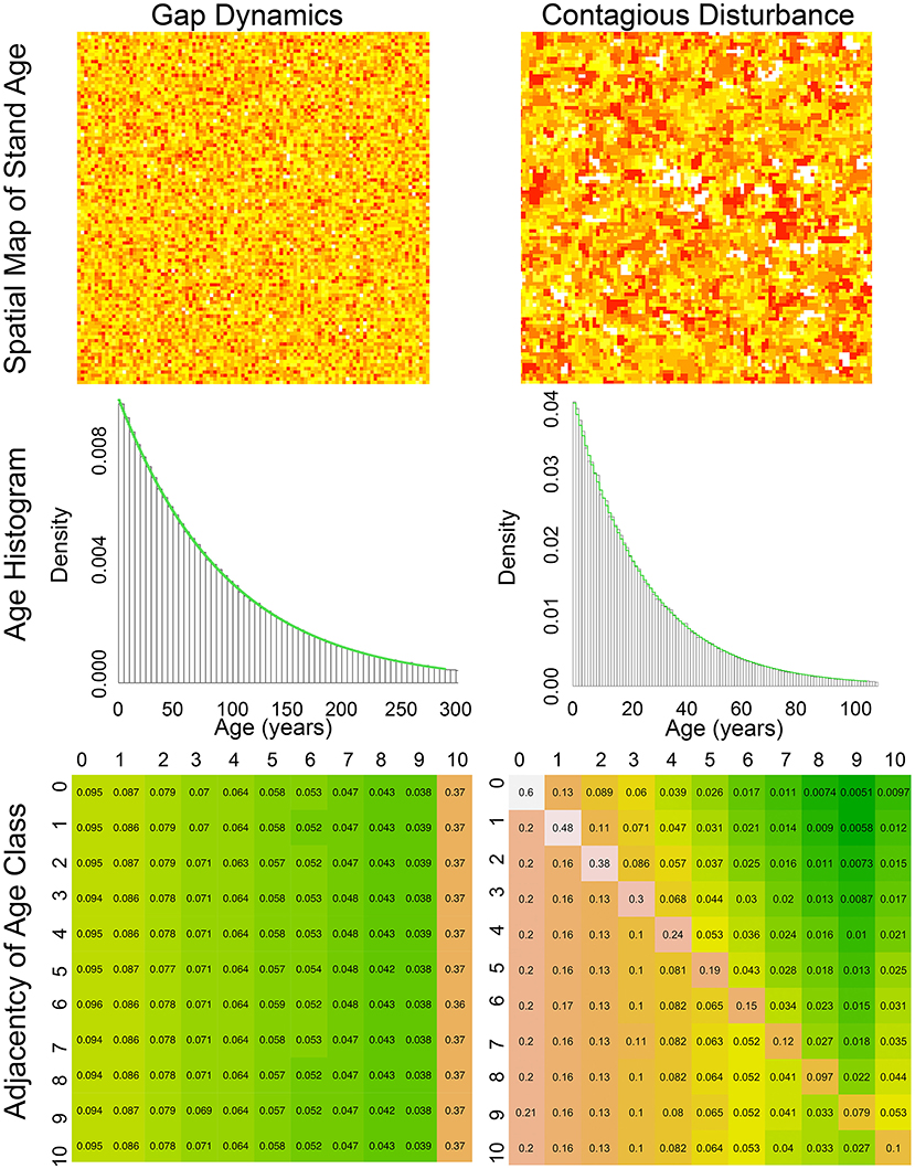
Figure 1. Comparison of Gap dynamics Contagious disturbance simulation. (Left column) Gap dynamic simulation. (Right column) Contagious disturbance simulation. (Top left) spatial map of stand age, with color on a log scale from youngest (red) to oldest (yellow), (Top right) spatial map of stand age for contagious disturbance, with color on a log scale from young (red) to old (yellow) and with new disturbances (age = 0) in white. (Middle left) simulated stand age distribution (black) when disturbance probability is 1% compared to geometric expectation (green), (Middle right) simulated stand age distribution (black) when disturbance probability is 1% and spread probability is 25% compared to geometric expectation (green), (Bottom) spatial adjacency matrix by age class aggregated into 10 year bins ([0−9] = 0, [10−19] = 1, etc.) with all patches 100 year or older in bin 10. Matrices are colored from white (highest adjacency) through orange to green (lowest adjacency).

Compare this gap dynamics model with a simple model of a contagious disturbance (e.g., fire, insects, land use), which is described first by a probability of disturbance initiation and second, conditional on initiation, a probability of spread to adjacent patches. In more complex versions of such models both these probabilities can vary with age and environmental conditions (Mann et al., 2012). However, even in the simplest case, when both probabilities are fixed and disturbances are random, the model generates much more complex spatial patterns characterized by larger, contiguous disturbance patches (Figure 1 right). As before, the overall stand age distribution remains geometric (Figure 1 mid right), however the pattern of spatial adjacency is more complicated (Figure 1 bottom right). First, most newly disturbed patches (age class 0) are adjacent to other newly disturbed patches (60% in the example simulation). As we move along the diagonal of the adjacency matrix, patches in a given age class continue to remain adjacent to other patches of the same age through time (i.e., larger even-aged patches remain), but this adjacency decays geometrically as new disturbances chip away at even aged patches, leaving them adjacent to younger disturbances. Above the diagonal we see a pattern similar to gap dynamics, where each age class has some probability of being adjacent to newly disturbed patches (which in this simple class is equal for all age classes) and then this adjacency decays equally for each age class. Matrix elements that are below the diagonal, which represent the probability that a patch is adjacent to a patch older than it, age classes likewise decay geometrically, but each age class is along a different curve because of the different cumulative probabilities. In other words, because the elements along the diagonal differ for each age class, and because the cumulative probabilities must sum to 1, the remaining cumulative probability is different for each age class.

Armed with a basic understanding of the patterns that spatially explicit simulations can produce, let us next consider how to develop a spatially implicit model to approximate the spread of contagious disturbance. As in the simulation, let us start by assuming an age or stage structured approach with n discrete age classes. Next, let us assume that the disturbance has some initiation probability, p₀, that is a vector with the same length as the number of age classes, n. In other words, the initiation probability could vary by age class. In this general derivation, our timestep or “t” represents any discrete timestep (annually, monthly, etc.). Because disturbance is simulated discretely in time, the probabilities map to that timestep and can be time varying (e.g., functions of environmental conditions) without loss of generality.

Given this initiation probability, the initial disturbance area (for disturbances with size = 1 patch) is given by I₁ = p₀°a, where a is a vector of the fractional areas of each age class and ° denotes element-wise Hadamard multiplication. Next, let us assume that we know the current adjacency matrix, A_t, that describes the probability that a patch of a given age/stage class is adjacent to patches of the same or other age/stage classes at time t. Individual elements within A_t are probabilities, and thus must be between 0 and 1, and all patches must be adjacent to some other patch so each row represents a discrete probability distribution whose elements must sum to 1. However, A_t does not need to be symmetric (e.g., Figure 1 bottom right). In practice the specification of these probabilities will depend on the spatial grain of the analysis (i.e., patch size) but this does not affect the mathematical derivation. Also, in practice the initial adjacency, A₀, would need to be derived from some sort of empirical GIS analysis or some steady-state assumption but this does not affect the derivation. Finally, except when deriving the dynamics of updating A_t+1 given A_t we will drop the time subscript for simplicity, as we are not considering changes in A during a disturbance event.

To allow contagious disturbances to spread we also need to introduce a probability of spread, p_s, given initiation, which similar to I₁ is grain and timestep dependent and could be time varying. In the general case we will assume p_s is a n×n matrix describing the probability of spreading from one class into any other class, but in practice p_s could be a scalar or set to only vary by row (dependent on the class the disturbance is spreading from) or column (dependent on the class being spread into). It should also be noted that p_s does not need to be symmetric—the probability of spreading from one patch type into another (e.g., new regeneration into old-growth) need not be the same as the probability of spreading back. Given this framework we can next derive the probability of a disturbance spreading to a second patch as depending on initiation, probability of spread, and adjacency:

$I_2=(p_s\circ A)I_1$

Furthermore, we can see that I₃ = (p_s°A)I₂ and so on, leading to the more general recursion describing the probability of spreading to h + 1 patches, given that the disturbance has already spread to h patches.

$I_{h+1}=(p_s\circ A)I_h=S{I}_h=S^h{I}_1$

Where S = p_sA. Note that in this derivation the matrix A is fixed as it describes the adjacencies among the undisturbed age classes; the ongoing disturbance is not an explicit row/column in A and thus spread only occurs outward into undisturbed area, and there is no need to account for the spread of a disturbance backward into patches that were just disturbed. We also make the simplifying assumption that we are operating on a sufficiently larger scale that no single disturbance event changes the adjacency among undisturbed patches enough to invalidate this approximation (and require updating A during a disturbance event). That said, adjacency does need to be updated on our coarser model timestep as what we generally see is small year-to-year changes that gradually accumulate to appreciable landscape-scale adjacency shifts over longer time (e.g., decades).

Accumulating the spread over different disturbance sizes leads to an overall disturbance rate of

$\begin{array}{l}D={\displaystyle \sum _{h=1}^{\infty }}{I}_h\end{array}$

where D is a vector by class. Overall, while there is slight underestimation of disturbance extent at high spread probabilities (Figure 2), the analytical approximation performs well and incurs a tiny computational cost relative to spatially explicit models. Also note that this general forward model has an important special case, p_s = 0, which corresponds to non-contagious disturbances, such as our initial gap dynamics simulation.

FIGURE 2

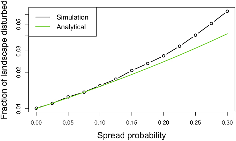
Figure 2. Validation of the analytical model's ability to predict disturbance area as a function of spread probability (disturbance initiation probability of 1%). Simulations run on a 4-sided grid so, for example, a 0.25 spread probability corresponds to four independent chances, each 25%, to spread. The analytical approximation appears to underestimate disturbance at high spread probabilities.

In practice an infinite sum is not actually computable, but the result will asymptotically approach the analytical result and thus can be approximated with a finite sum. Furthermore, the relative proportions of the different age/stage classes within the ith iteration in the sum (i.e., disturbance of size i), I_i, will rapidly approach a steady-state distribution. If $I_i/\sum I_i\approx \frac{I_{i+1}}{\sum I_{i+1}}$ then we approximate I_i+1 = I_iS with I_i+1 = I_iλ where λ is the dominant eigenvalue of A. The remainder of the summation $\sum _{h=i+1}^{\infty }{I}_h$can thus be approximated as $I_i\sum _{h=i+1}^{\infty }{\lambda }^{h-i}$. This is just a geometric series, which has the analytical solution $I_i\lambda {(1-\lambda )}^{-1}$. Therefore, our strategy is to solve the first i terms explicitly and analytically approximate the tail of the distribution

$\begin{array}{l}D={\displaystyle \sum _{h=1}^i}{I}_h+I_i\lambda {(1-\lambda )}^{-1}\end{array}$

As seen in Figure 3, this allows the full analytical model to be accurately approximated with only a small number of matrix multiplications (~5 in this scenario)

FIGURE 3

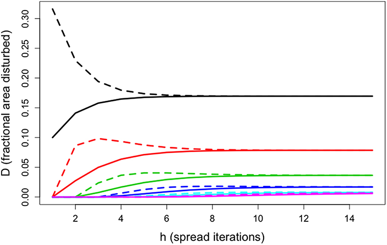
Figure 3. In this scenario, disturbance was initiated in one class (black) at 10%, and then spread to other classes (spread probability of 25%) based on differing probabilities of adjacency between classes (50% self-adjacency, 50% adjacent to the next class). Solid and dashed lines are a comparison of how cumulative area disturbed increased with disturbance size for both the full model and the tail approximation (estimator).

Dynamic Updating

Fractional Areas

Once the overall disturbance rate, D, has been calculated we need to update both the fractional areas describing the landscape and the adjacency matrix between those fractional areas. First, let us assume that a_t = [a₀a₁…a_n−1a_n] is a vector describing the fractional areas of each of our age classes. Let us also assume that all disturbances reset patches to age class 0, which is the conventional assumption in cohort-based vegetation demography models (Moorcroft et al., 2001; Fisher et al., 2018; VDMS). Note that we are not assuming that disturbance removes all of the vegetation and that age class 0 is bare ground, but rather we are using age 0 to semantically indicate 0 years since last disturbance. Following this assumption, the new fractional area in age class 0 at time t+1 is simply the sum of the disturbance rates in each age class times the current fractional area in each of those age classes, $a_{0,t+1}=\sum _{k=0}^n{a}_{k,t}{D}_{k,t}$. Next, for all other age classes, each age class ages by 1 year and is reduced by the amount of disturbance that occurred in that class

$\begin{array}{l}{a}_{k,t+1}=a_{k-1,t}(1-D_{k-1,t})\end{array}$

Finally, the oldest age class is a special case, representing all stand equal or greater than the specified age, and thus is created by fusing the existing area in that class with the next youngest age class, minus the disturbance occurring in each

$\begin{array}{l}{a}_{n,t+1}=a_{n-1,t}(1-D_{n-1,t})+a_{n,t}(1-D_{n,t})\end{array}$

Adjacency of Newly Disturbed Patches

In addition to updating the fractional areas in different age classes we also need to be able to update their adjacencies. This updating is done after the disturbance events of a given time-step, not as part of the disturbance simulation itself. This distinction means that the adjacency at a timestep (A_t) is not tied to a disturbance but rather represents the cumulative effects of disturbance on the landscape over a timestep.

Let us start by focusing on the adjacency of the newly disturbed age class, a₀, with itself, which we will denote as A₀₀. If we were assessing this adjacency in a spatially-explicit gridded dataset or simulation, we would estimate the probability of adjacency in terms of the frequency with which disturbed patches are adjacent to other disturbed patches vs. non-disturbed patches. For example, for a disturbance of size 1, all four edges are facing non-disturbed patches, so the adjacency is 0/4 = 0 (Figure 4). With a disturbance of size 2, the two patches have a total of eight edges, two of which are on the interior of the disturbance (disturbed patch adjacent to disturbed patch) and six external edges that are along the perimeter of the disturbance, giving an adjacency of 2/8 = 0.25. At size 3 there are two possible disturbance configurations (in a line or an L), but both cases have a total of four interior edges and eight external edges, giving an adjacency of 4/12. At size 4 there are five possible configurations, and the different configurations do not all have the same perimeter—the square configuration has an adjacency of 8/16 while all other configurations have an adjacency of 6/16. If disturbance shapes are completely random then we could work through the combinatorics of how often each shape is likely to occur (squares occur 20% of the time) and calculated a weighted average (0.4). More generally, if we look at the whole map across disturbances of different sizes the overall mean adjacency of disturbed patches will be

$\begin{array}{l}{A}_{00}=\frac{\sum Int}{\sum Int+\sum Ext}\end{array}$

where Int are interior edges and Ext are external edges.

FIGURE 4

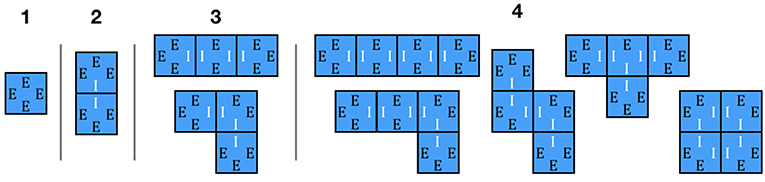
Figure 4. Adjacency for small disturbances. Edges are labeled as (E)xterior and (I)interior. For size 1, there is 0 probability of self-adjacency (disturbed patches adjacent to other disturbed patches). For size 2 and 3 it is 1/4 and 1/3, respectively, while for size 4 the adjacency is either 1/2 (square configuration) or 3/8 (all other configurations).

Thus, far we have seen that the adjacency (interior/total edges) has tended to increase as the size of the disturbance increases. We could continue calculating this pattern to larger disturbances with more complex shapes and harder combinatorics (e.g., for a size 5 disturbance there are 372 possible spread scenarios that produces thirteen possible shapes). However, at this point it is worth noting that different types of disturbances may be more likely to produce certain disturbance shapes than others. For example, some disturbances may tend to produce shapes that tend to be round (wildfire) while others might tend to be linear or dendritic (urban development, riverine systems). These different shapes tend to produce different characteristic interior/total ratios (i.e., different adjacencies). However, it is not the overall mean adjacency (interior/total) that characterizes a disturbance, nor any of the many other landscape metrics in use (e.g., Maximillian et al., 2019), but the functional relationship between disturbance size and adjacency, adj (size). For example, Figure 5 shows the adjacency/size curves for three important cases: random spread (purple), the minimum adjacency (blue) achieved through linear disturbances, and the maximum adjacency (red) achieved by circular disturbances that minimize the interior:total ratio.

FIGURE 5

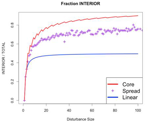
Figure 5. Self-adjacency as a function of disturbance size for different disturbance shapes. Core and Linear are the bounding cases of disturbance shapes that maximize and minimize self-adjacency (respectively). Spread is a single realization of the stochastic contagious spread model (Figure 2).

To get the overall A₀₀ for the spatially implicit model, we next replace

$\begin{array}{l}{A}_{00}=\frac{\sum Int}{\sum Int+\sum Ext}\end{array}$

which sums over individual disturbances, with

$A_{00}=\frac{{\displaystyle {\sum }_{size}Int(size)p(size)}}{{\displaystyle {\sum }_{size}Int(size)p(size)+{\displaystyle {\sum }_{size}Ext(size)p(size)}}}$

which instead sums over each disturbance size. In this approximation, Int(size) and Ext(size) returns the expected number of interior and exterior edges while p(size) is the probability of a disturbance of that size. In the denominator we can combine terms as $\sum _{size}(Int(size)+Ext(size))p(size)=\sum _{size}4·size·p(size)$ where the 4 arises from the assumption that patches are 4 sided. The size distribution itself can be calculated from the series of I_k, p(h) = (I_h−I_h+1)·h, because I_h represents the probability of observing a disturbance of size greater or equal to size h+1. Differencing gives us the probability of a disturbance size h occurring, which is then multiplied by the disturbance size to give us the probability of encountering a disturbance of that size (e.g., the disturbances that stayed size 1 are the subset of disturbances that were initiated but did not spread to another grid cell). Finally, just as we truncated the calculation of D in section Simulating Disturbance Spread, the tails of this distribution can be approximated by noting that the geometric series implies a geometric PDF with rate λ. In the numerator we can use our previously discussed relationship between adjacency and size class, adj(size) to calculate Int(size) = 4·size·adj(size). Putting these together we see that the assumption about the number of sides to a patch cancels out leaving us with just the mean adjacency weighted by disturbance size and the disturbance size probability distribution

$A_{00}=\frac{{\displaystyle {\sum }_{size}adj(size)\cdot size\cdot p(size)}}{{\displaystyle {\sum }_{size}size\cdot p(size)}}$

This derivation makes sense because large disturbances should contribute more to the adjacency, but usually occur at lower probabilities. Our derivation states that the second-order spatial scaling of any disturbance regime can thus be understood in terms of its size distribution and adj(size). In the analysis of empirical disturbances section, we will evaluate these two components empirically for different disturbance types and ecoregions in Florida and Oregon. In evaluating this approach against simple simulation models, we discovered an important inconsistency in the model, as independent disturbances do sometimes end up adjacent to each other by chance. Consider again our earlier example of simulating gap disturbance (p_s = 0). In this case there is no spread, and thus our adjacency-based model makes the prediction that all disturbances are size = 1, and thus A₀₀ = 0, but in practice we find adjacent disturbances. To correct our model, we thus added an additional term in the numerator that accounts for the adjacency between independent disturbances. The simplest such correction is to assume that other disturbances are encountered randomly at the overall disturbance rate, a₀.

$\begin{array}{l}{A}_{00}=\frac{{\displaystyle {\sum }_{size}Int(size)p(size)+{\displaystyle {\sum }_{size}{a}_{0}Ext(size)p(size)}}}{{\displaystyle {\sum }_{size}Int(size)p(size)+{\displaystyle {\sum }_{size}Ext(size)p(size)}}} \\ A_{00}=\frac{{\displaystyle {\sum }_{size}\left[adj(size)+a_0(1-adj\left(size\right))\right]·size·p(size)}}{{\displaystyle {\sum }_{size}s}ize·p(size)} \end{array}$

The adjacency predictions corrected to account for this random self-adjacency performed well (Figure 6).

FIGURE 6

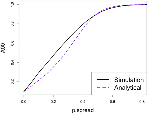
Figure 6. Validation of the ability of the analytical approximation to predict self-adjacency of newly-disturbed patches as a function of disturbance spread probability (disturbance initiation probability set to 10%).

Adjacency of Non-disturbed Patches

In addition to needing to update the adjacency of disturbed patches to each other, there are three other cases that need to be considered: the adjacency of newly disturbed patches to non-disturbed, the adjacency of non-disturbed to newly disturbed, and the adjacency of non-disturbed to each other. For these cases we are going to make the simplifying assumption that the adjacency in each age class changes in proportion to the disturbance rate in that age class, D_k. This assumption is likely reasonable when spread rates are similar among age classes, but very large differences in spread rates, or large asymmetries in spread direction, could be tested through a detailed accounting of the adjacency, A, and spread, p_s, at every disturbance size, I, and age class, k. Doing so would come at the expense of considerably more complicated accounting and notational complexity, and thus this is left to future work.

For the first case of disturbances adjacent to non-disturbances, we want to normalize D by its sum to generate the probability that the disturbance was in that age class. As with the age-class distribution, we also want to shift the age classes by 1, to account for aging, and sum the final two elements in this vector to account for age-class fusion. Next, because rows sum to zero this vector of probabilities needs to be reduced by 1−A₀₀, giving

$\begin{array}{l}{A}_{0k,t+1}=\frac{D_{k-1}}{\sum D}(1-A_{00,t+1})\end{array}$

Next, consider the case of non-disturbed patches adjacent to other non-disturbed patches. Here the adjacency should be reduced by the amount of disturbance in that age class, which is the disturbance rate normalized by the fractional area.

$\begin{array}{l}{A}_{j,k,t+1}=A_{j-1,k-1,t}(1-D_{j-1}/a_{j-1})\end{array}$

As before, age classes are shifted by 1 and the final two classes are merged, however in this case the merge is an average (weighted by fractional area), rather than a sum.

Finally, because rows sum to 1, the adjacency of non-disturbed to newly disturbed patches are one minus the sum of the other elements in the row

$\begin{array}{l}{A}_{j,0,t+1}=1-{\displaystyle \sum _{k=1}}{A}_{j,k,t+1}\end{array}$

To test the performance of the analytical adjacency approximation, we compared the adjacency matrix predicted by this model to that generated by a fully spatial stochastic simulation, analogous to the one shown in the right column of Figure 1 but with a disturbance initiation probability of 1% and a spread probability of 10%. In both the analytical model and stochastic simulation, we initiated the landscape from bare ground (age = 0) and ran the model for 1,000 years to reach a steady-state.

Analysis of Empirical Disturbances

Data Description

Our analysis looked at disturbances in Oregon and Florida from the LANDFIRE Disturbance product (Earth Resources Observation and Science Center, U.S. Geological Survey) for 2014, the most recent year available. Florida and Oregon were chosen as contrasting disturbance regimes because they are both areas with fire-based disturbance regimes and a large timber industry (Fox et al., 2007; Marlon et al., 2012; Mitchell et al., 2014). The LANDFIRE disturbance product is a 30 × 30 m resolution gridded raster covering the entire US, with each disturbed cell assigned one of twenty different disturbance types. Disturbances were determined by a combination of LANDSAT satellite imagery, MODIS satellite imagery, vegetation change detection techniques, and a database of disturbance events detected by other federal agencies (Rollins, 2009; Vogelmann et al., 2011). Specifically, the 2014 LANDFIRE Disturbance dataset was constructed with best-pixel composite imagery, other composite imagery, or majority focal filling to account for missing data after the decommissioning of LANDSAT 5. In our analysis we treated the LANDFIRE Disturbance product as given, and did not consider associated levels of uncertainty within different disturbance types and pixels.

We downloaded US state data from the LANDFIRE repository, available at https://landfire.cr.usgs.gov/disturbance_2.php. The authors then subset Disturbance dataset for each US state based on and Environmental Protection Agency level II Ecoregion boundaries (Ecoregions; McMahon et al., 2001). Subsetting was done using with the R raster and rgdal packages (Hijmans, 2017; Bivand et al., 2018). We subset the US state-level rasters to focus on the two forested level II ecoregions within each state: Mississippi Alluvial and Southeast Coastal Plains (8.5) and the Southeastern USA Plains (8.3) in Florida; and the Western Cordilleras (6.2) and Marine West Coast Forest (7.1) in Oregon. In Oregon we excluded the Cold Deserts ecoregion (10.1) and in Florida we excluded the Everglades (15.4) (Figure 7). The resulting four rasters then had adjacency calculations done on all of the disturbance clumps within each raster (see below).

FIGURE 7

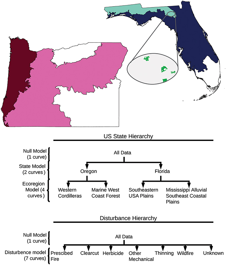
Figure 7. Visualization of data subsetting and model hierarchies. Colored regions show what portions of Oregon and Florida were used in analyses. Cutouts show a sample of LANDFIRE raster file with disturbances in green. Model hierarchies show the different models compared, and the data used to make each curve.

Calculation of Metrics

The analysis of empirical disturbances focused on the two metrics that emerged from our theoretical model: disturbance size distribution and the relationship between interior ratio and disturbance size. The analysis began by identifying individual disturbances that were surrounded on all sides by non-disturbance pixels. Adjacency was determined using the four cardinal “Rook's Case” pixels (for two pixels to be adjacent they had to share a side). For each disturbance we then identified the disturbance class and calculated the disturbance area and interior ratio (number of interior edges/total number of edges, Figure 4). After processing the four rasters, we ended up with a table of each disturbance event in Florida and Oregon, with a record of its type, size, interior/total ratio, eco region, and US state. This table is the basis of all further empirical calculations and is publicly available along with the scripts used to generate it on Github at https://github.com/mccabete/SpatialAdjacency. This analysis has no way of distinguishing distinct but adjacent disturbance events that occurred at different times within a year, therefore these distinct but adjacent disturbance events were considered the same clump. This analysis also did not account for relative area of different disturbance types mixed within a single clump. Clumps of mixed disturbance types accounted for a small number of disturbance events (1%), but a large fraction of disturbance area (56%) (Figure 9; Supplemental Table 1). We treated Mixed disturbance as a separate class of disturbance in our comparison of size distributions. To calculate interior ratio curves these mixed disturbances were removed. Many of the disturbances most frequently co-occurring within mixed disturbances are represented in our curve fits (Supplemental Figure 2).

Assessing Statistical Significance

We used two different statistical tests for the two different disturbance metrics. For the size distributions, we compared the size distributions of disturbance type, US states, and ecoregions using a two-sided Kolmogorov–Smirnov test. We corrected the P-values using a Bonferroni correction (Massey, 1951; Bland and Altman, 1995). We compared size distributions of all disturbance types present within Florida and Oregon that had 20 or more disturbance events. This excluded biological and disease disturbance classes (N = 4, N = 6; Supplemental Table 1). We made 66 pairwise comparisons among 12 disturbance types, and three comparisons among state and two ecoregions. After correction, our alpha value was 0.000725 (Supplemental Table 2).

For the interior to total ratio, we fit and statistically compared curves corresponding to null models and different hierarchy levels. The curves were fitted using a modified Michaelis-Menten curves of the form $y=\frac{a{x}^c}{b+x^c}$ using a maximum-likelihood approach assuming Gaussian error (Michaelis and Menten, 1913). The form was chosen based on visual agreement with the data and maximum likelihood after comparison with six other functional forms (Supplemental Figure 1; Supplemental Table 3). Different curves were compared using a likelihood ratio test. Comparing the curves meant comparing different hierarchical levels (Figure 7). We fit two hierarchies, one starting at the US state level, and one at the disturbance-type level (Figure 7). In the US state hierarchy, an all-data null model was compared to a model where Oregon and Florida were fit separately. The US state-model was then compared to a model where each ecoregion was fit separately. In the second hierarchy, an all-data null model was compared to a model where each disturbance type was fit separately. The disturbance-model was then compared to a disturbance-by- US state model (Figure 7; Supplemental Table 4). We also separately compared a one-curve-Florida model to a two-curve-ecoregion model, and a one-curve-Oregon model to a two-ecoregion-curve model. We did this to see if the differences between ecoregions within Florida would be significant in isolation of the differences between Oregonian ecoregions (Supplemental Table 4). Because all single-pixel, double-pixel, and triple-pixel configurations produce the same interior ratio (Figure 4), curves were fit only to disturbances over 3 pixels (0.27 ha) large. To meet requirements of likelihood ratio tests, the data was subset to include only the disturbance types that were common amongst all ecoregions. Disturbance types included: clearcut, herbicide, other mechanical disturbances, prescribed fire, thinning, wildfire, and unknown. The distinction between wildfire, and prescribed fire is that a wildfire is an unplanned fire, prescribed fires are intentionally set and managed fires (LANDFIRE Disturbance, 2016). To contextualize modeled curves, we included hexagonal density plots, representing the spread and overall shape of all the data used to generate curves (ggplot2, 3.0.0; Wickham, 2016). To aid in interpretation, the upper and lower bounds for the interior ratio were also visualized based on calculations of the theoretical minimum (linear disturbance) and maximum (round disturbance) interior ratios for a given disturbance size. All analyses were performed in R (3.5.0; R Core Team, 2018) with adjacency calculations performed using the raster library (2.6-7; Hijmans, 2017).

Results

Dynamic Adjacency Updating

The analytical model for calculating disturbance spread and dynamically updating landscape adjacency was assessed by comparing the analytical model to a spatially-explicit stochastic simulation. In both cases the landscape was initiated from bare ground (age = 0) and run 1,000 years to reach a steady-state. Figure 8 shows that the steady-state adjacency predicted by both models had the same structural features, as summarized in section Simulating Disturbance Spread: patches within an age class tended to be more self-adjacent, but that self-adjacency decays geometrically with age; there is also a geometric decay along rows, but with greater adjacency above the diagonal. Numerically, the predicted adjacencies were also very similar, though with the analytical model slightly overpredicting A_{0, 0}. Because so many of the other rates in the adjacency matrix decay from A_{0, 0}, there are slight biases elsewhere. However, the error propagation from A_{0, 0} is consistent with the underlying structure for updating the matrix being correct, because it means that structural elements are preserved as the landscape ages.

FIGURE 8

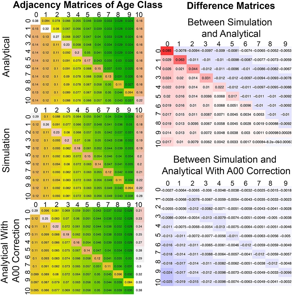
Figure 8. Comparison between adjacency matrices for a stochastic spatial simulation (simulation from Figure 2, middle) analytical approximation (top), and analytical approximation where a correction was applied to A00. All adjacency matrices are after 1,000 years (steady state). To the right are difference matrices between the simulation matrix and the two analytical matrices. Age class aggregated into 10 year bins ([0−9] = 0, [10−19] = 1, etc.) with all patches 100 year or older in bin 10. The 10th column of the error matrices was removed because of a summing to 1 constraint.

This impact of errors in A_{0, 0} on the overall adjacency calculation was tested with a third model (Figure 8 bottom left), where the analytical model was run using the A_{0, 0} derived from the numerical simulation. Overall this model improved the overall pattern in the adjacency matrix, especially along the main diagonal. The remaining error (Figure 8 bottom right) is largely concentrated in two places. First, there is greater adjacency with the oldest “absorbing” age class than observed in the simulation (left hand column). Second, because of this the bottom left corner (adjacency of old age classes to young classes) is a bit lower than observed. Matrix rows have a sum-to-one constraint, so some of these errors are inevitable compensating errors. It is also worth noting that in nudging A_{0, 0} directly we are not nudging the underlying terms used to calculate A_{0, 0} (I, D, a), which are also used in update the rest of A, meaning this test is not strictly internally consistent. An open question is how much of the remaining error in the adjacency matrix updating, is in the underlying analytical simulation of disturbance spread (I, D, a) vs. approximations in the updating of A? This is something we hope to investigate further in the future.

Disturbance Size Distribution

Our Kolmogorov–Smirnov pairwise comparison of disturbance type size distributions found that the majority of disturbance types had significantly distinct distributions (p < < 0.001) (Figure 9; Supplemental Table 2). The three exceptions were clearcut, wildland fire, and harvest, which had non-significant differences with roughly half of the disturbance classes. Finally, mastication had no significant difference between wildfire and chemical (Supplemental Table 2). The size distributions of Florida and Oregon were significantly different, as well as the two ecoregions nested within Oregon (p < 0.001; Supplemental Table 4). The two ecoregions size distributions nested within Florida were not found to be significantly different. However, in other size distributions significant differences were found despite visual similarity in part due to large sample sizes. The size distributions have a large range in sample sizes. US state-level size distributions were based on very large sample sizes (Oregon N = 27,137, Florida N = 20,329). Disturbance sample sizes range from harvest with N = 22 to unknown N = 34,560 (Supplemental Table 1). Unknown disturbances accounted for the majority of disturbance events in the overall dataset, and a large proportion of the area (20%). All four ecoregions had a similarly shaped size distribution, with peaks at single-pixel (0.09 ha) disturbances and at 7 ha disturbances. The 7-ha peak aligns with disturbance peaks in the disturbance categories unknown, thinning, wildland fire, mixed, harvest and wildfire. Within Oregon, the Western Cordillera ecoregion has more small and mid-level size disturbances than the Marine West Coast Forest, the Western Cordillera also had both considerably more disturbance events than the Marine West Coast Forest, and a larger area of disturbance (75%). Disturbance plots show more varied patterns, Wildfire and prescribed fire have a long tails, reflecting the influence of rare but large disturbances. In contrast, thinning and mastication have distinct peaks and sharper drop-offs, suggesting more standardized anthropogenic disturbances and smaller sizes. Mixed disturbance has the longest tail, and no peak at small disturbances. Herbicide and other mechanical disturbances have visually similar distributions but were found to be significantly different (Herbicide N = 4,655, Other Mechanical N = 3,546). Within mixed disturbances, herbicide and other mechanical disturbances co-occurred most frequently (Supplemental Figure 2).

FIGURE 9

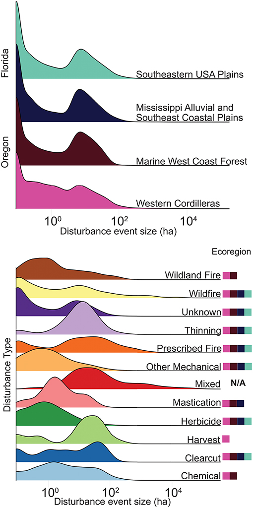
Figure 9. Size density plots showing the contrasts between ecoregion/state and disturbance type. Colored boxes next to disturbance size density curves show what ecoregion contains the respective disturbance. Sample sizes associated with density plots can be found in Supplemental Table 1.

Disturbance Interior Ratio Curves

We found a significant effect of US state (p < 0.001) and ecoregion nested within states (p < 0.01). Oregon had a wider range of interior ratios, with a higher occurrence of linear disturbances than Florida (Figure 10). Florida and Oregon have similar numbers of overall disturbance occurrence, but Oregon disturbances have a larger proportion of the total area of disturbances (%79). Within Oregon, small disturbances were more compact in Marine West Coast forests than in the Western Cordillera small disturbances, but this relationship crosses, such that Marine West Coast disturbances were less round at large disturbance sizes. The curves fit for the two ecoregions in Florida are nearly identical (Figure 10). Despite visual similarity, the two ecoregion curves were found to be significantly different even when compared to just a Florida curve model. Best fit parameters for all curves are provided in Supplemental Table 5.

FIGURE 10

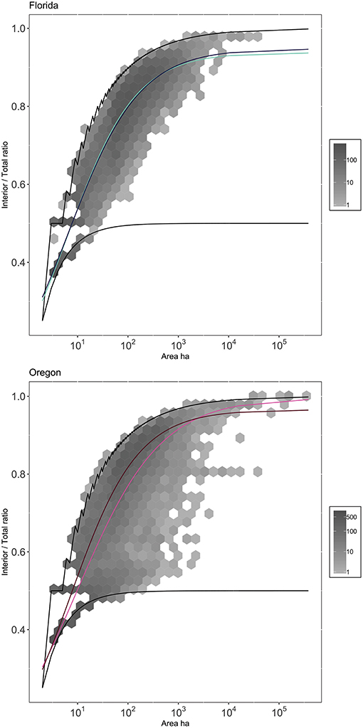
Figure 10. Mean trends of Ecoregion within State. Curves match Ecoregion model curves referenced in Figure 7. Gray hexes correspond to binned-counts of number of disturbance events. Black lines correspond to core and linear bounding cases. Parameter values associated with curves can be found in Supplementary Table 5.

In our second hierarchy, there was a significant effect of disturbance type (p < 0.0001), but not US state nested within disturbance (p > 0.1). Herbicide is the most distinctively linear, followed by other mechanical disturbances, and then unknown disturbances. Fire disturbance types (prescribed and wildfire) were closer to the maximum interior ratio curve, suggesting that fires tend to be compact and burned pixels were predominantly adjacent to other burned pixels (Figure 11). Disturbance-level curves show that prescribed fires are less compact at smaller sizes and larger sizes than natural fires, but at the most frequent size is similarly shaped. Thinning resembles other compact disturbances, but begins to become more linear at large sizes relative to wildfire. Clearcut follows a similarly compact pattern to wildfire. Individual disturbance curves and data plots can be found in the supplement (Supplemental Figure 3).

FIGURE 11

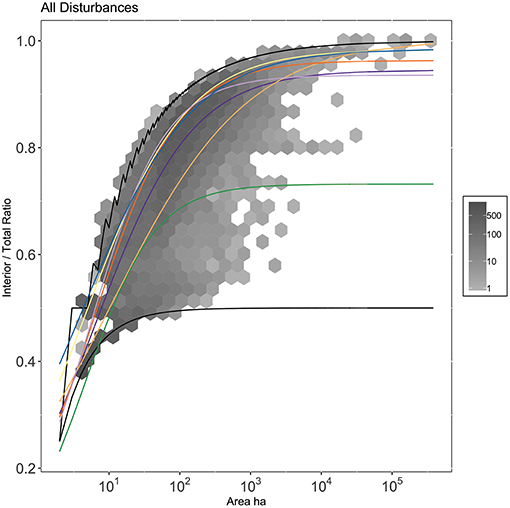
Figure 11. Mean trends of disturbance type. Curves match Disturbance model curves referenced in Figure 7. Gray hexes correspond to binned-counts of number of disturbance events. Black lines correspond to linear bounding cases. Parameter values associated with curves can be found in Supplementary Table 5. Plots of individual curves against data can be found in Supplementary Figure 3.

Discussion

Theoretical Framework

Our framework for scaling spatially-implicit contagious disturbances is reasonably accurate, computationally efficient, and theoretically provocative. Our framework was able to estimate the fraction of the landscape that was disturbed as a function of disturbance initiation, adjacency, and spread probabilities (Figure 2). We were able to show that disturbance initiated in one age class would spread into stands of different ages based on their relative adjacencies (Figure 3). We demonstrated not only the ability to predict the self-adjacency of newly-disturbed areas (Figure 6), but also the adjacency of newly-disturbed areas to non-disturbed areas and the ability to update the adjacency of non-disturbed areas to each other in light of new disturbance. While the corrected self-adjacency predictions perform well (Figure 8), improving this correction is a useful area for future research, for example by accounting for the size of disturbed patches in calculating the probability that they will merge. In addition, it is important to note that when simulating disturbance using empirical adj functions that this correction term does not need to be included unless distinct, but adjacent, disturbances occurring during the same time step, were separated in the original data (usually this is not possible). We were able to successfully update adjacency over 1,000 years within a reasonable level of accumulated error, and capture the major emergent features of contagious disturbance adjacency (Figure 8), such as the geometric decay of self-adjacency as even-aged stands mature and the geometric decay of adjacency within an age class (greater probability of being adjacent to newer disturbances) with greater adjacency above the diagonal (young) than old. That said, if older age classes are aggregated (bottom row) then considerable self-adjacency among old-growth stands can develop.

There are a number of important applications where this modeling framework can be immediately applied and expanded upon. At the top of this list is improving the incorporation of sub-grid scale disturbance processes within regional and global scale models, such as Dynamic Global Vegetation Models (DGVMs), Vegetation Demographic Models (VDMs, Fisher et al., 2018), and coupled Earth System Models. These models operate at a scale where spatially-explicit approaches are not computationally feasible– a typical landscape model operating at LANDSAT (30 × 30 m) resolution would require simulating hundreds of billions of grid cells to capture the Earth's land surface. As a result, disturbances that we know to be spatially contagious are either absent from these models altogether (Hicke et al., 2012; Dietze and Matthes, 2014; e.g., insects and pathogens) or represented using much simpler zeroth-order (spatially homogeneous) or first-order (fractional area) approximations (e.g., fire, land use). By using these simpler approximations, existing models miss important ecological phenomena, such as the spread of disturbance initiated in one age class or vegetation type into other vegetation within that grid cell. Depending on whether these models assume fractional areas are completely independent or randomly-distributed, these approaches will systematically either over- or underestimate (respectively) the degree of spatial adjacency occurring on the landscape. This will potentially bias estimates of dispersal limitation, lateral shading, microclimate, and lateral hydrologic and biogeochemical fluxes (Melton and Arora, 2014).

Even where spatially-explicit models are computable (e.g., landscape-scale models of vegetation communities and biogeochemistry), there is often considerable uncertainty in the initial conditions. Spatially explicit models require state variables to be estimated at a fine spatial resolution (Shifley et al., 2008), which is very data intensive and frequently underconstrained. Furthermore, the errors in spatial maps of initial conditions are not independent, so the uncertainties do not simply average out with the number of grid cells. In contrast, with spatially-implicit models we can often generate estimates of the probability distributions of age classes and their adjacency with much greater confidence (law of large numbers) than we can map explicitly. For example, one may be able to estimate the fraction of a landscape that is a certain age class (e.g., 10 to 20-years-old) much more precisely than one can estimate the age of a specific 30 × 30 m pixel. Because of this, the total predictive uncertainty in a spatially explicit model could be larger than a spatially-implicit approximation, for example if the initial condition uncertainties of the spatial model outweigh the approximation errors of the implicit model (Dietze, 2017). Without detailed inventory data, initializing a spatially explicit model presents a trade-off between feasibility and accuracy.

Beyond the global and vegetation modeling communities, our derivation can act as a null model for spatial processes like arrangement, location dependence, and absolute distance dependence. Arrangement can have an effect on certain contagious disturbances: for example, corridors can differentially affect seed dispersal dependent on angle relative to prevailing wind direction (Damschen et al., 2014). Habitat fragmentation can correlate with overall abundance of habitat, raising questions about the separability of configuration from size in occupancy modeling (Fahrig, 2002; Prugh et al., 2008; With and King, 2018). Absolute distance dependence is common in invasion ecology, where rare dispersal events over long distances can have a large effect on the subsequent colonization rates (Nathan et al., 2003). While some processes have spatial dependence that cannot be captured in our framework, the assumptions of our approach allow it to act as a non-trivial null-model to separate those effects (Rosindell et al., 2011). Explicitly accounting for size with adjacency is useful for disentangling the effects of size and arrangement, which often co-occur and can lead to misattribution (Prugh et al., 2008).

Empirical Analysis

In this analysis we characterized Oregon's and Florida's disturbance regimes based on their size distributions and the relationship between disturbance size and interior ratio. We hypothesized that these metrics would differentiate between contrasting US state-wide disturbance regimes and disturbance types, and would reflect the nested structure of ecoregions. Broadly, we found this to be true. Our interior ratio curves were able to significantly differentiate between US state, ecoregion, and disturbance types (Supplemental Table 4). In particular, different disturbances had characteristic interior ratio curves. Fire disturbances had compact configurations while several anthropogenically controlled classes (herbicide and other mechanical disturbances) spread dendritically. Relative to other mechanical disturbances and herbicide thinning spread in a compact way, but notably spread more dendritically at large disturbance sizes. This could indicate that thinning management strategies are fragmenting landscapes compared to natural disturbances. That said, the hierarchical structure of our analysis did not capture all possible permutations of lumping and splitting disturbance types, so similar curves (i.e., Clearcut and Wildfire; Figure 11) might have been lumped if evaluated independent of other disturbance classes. Overall, these results suggest that our metric captures the major features of the regions' disturbance regimes, and highlights the effects of anthropogenically mediated disturbances.

Size distributions of disturbances were generally distinct, but not sufficient to differentiate all disturbance types. That said, ecoregion-level size distributions had similar shapes (Figure 9). The consistent shape of the size distributions could be an artifact of the LANDFIRE disturbance attribution (Unknowns were the largest class of disturbance events) and could reflect the dominance of fire and thinning in both Florida and Oregon. Visually and statistically, the ecoregion size distributions support the nesting structure of the ecoregions: Florida ecoregions are more similar to each other than they are to the Oregon ecoregions (Figure 9; Supplemental Table 2). Disturbances reflect that high spreading probability creates larger disturbances: prescribed fire, wildland fire, and wildfire are the most long-tailed distributions (Figure 9).

Overall, a strength of this empirical analysis is that it describes disturbances in terms of size and of configuration separately, which contrasts with many spatial metrics which convolve the two (e.g., mean interior/total). That different sources of disturbance have different spatial patterns in disturbances alone is not an unexpected result. Intuitively, different disturbance mechanisms have different spatial signatures. A roadway-construction is smaller and narrower than a typical commercial thinning. These findings take that intuition a step farther and explore the patterns that emerge at larger scales. When an ecosystem's disturbance regime is changing, that change will manifest as changes to disturbance size, or disturbance configuration (the interior ratio curve), or both. In the future, if we characterize more disturbance regimes in terms of these metrics, and better understand what factors drive their variability in time and across large spatial scales, it should be possible to use these relationships to forecast the spatial scaling of changing disturbance.

As an example, consider a shift in disturbance regime that does not change the disturbance size, but shifts the shape from dendritic to compact. Dendritic disturbances create corridors through the landscape, which affects the demography of the ecosystem by changing migration, favoring certain dispersal mechanisms, and increasing the propagule pressure of certain areas. Size and shape of patch plays a role in the success of invaders (McConnaughay and Bazzaz, 1987; Fahrig, 2002). Dendritic disturbances alter the abiotic properties of a system through the creation of edges. Edge-effects have been found in forest systems to increase carbon uptake, increase available light, and increase nutrient deposition (Reinmann and Hutyra, 2017). At the other extreme, more compact disturbances could cause more evenly aged composition and introduce more within-patch homogeneity by having a larger fraction of the disturbed pixels “sheltered” from surrounding areas.

Many contagious disturbances are projected to change in magnitude, severity, and location with climate change (Flannigan et al., 2000; Bradley et al., 2010; Mitchell et al., 2014; Parks et al., 2016). Ultimately, these metrics will help us make concrete predictions of how to scale up these disturbances' regime changes. To be able to do this the variability within these metrics needs to be explored: How do they change year-to-year and place-to-place? How is this variability related to changes in weather, climate, and characteristics of the biotic and abiotic environment? This analysis demonstrates that interior ratio curves have the potential to communicate unique information about contagious processes and we encourage evaluating its utility in future work.

Opportunities and Challenges in Future Implementation

Implementing this spatially-implicit framework in real-world models requires that a number of inputs be derived through empirical analysis. First, the initial condition for adjacency, A_{t = 0}, needs to be estimated for every large-scale grid cell. Given maps of current vegetation, this is computationally intensive but a relatively straightforward operation either within GIS or scripting languages with geospatial libraries (e.g., R). Next, users need to then decide whether to forward simulate disturbances and interior ratios based on initiation probability and spread probability (section Simulating Disturbance Spread), or to rely on empirically observed size distributions and interior ratios (sections Disturbance Size Distribution and Disturbance Interior Ratio Curves). For short-term simulations, relying on empirically-derived statistics, such as those derived here for Florida and Oregon, is probably the easiest way to implement a wide range of different disturbance types. The empirical analyses conducted here could be further broken down using empirical covariates, such as weather, to capture changes interannual variability in disturbance size and shape (Hu et al., 2010). For longer-term simulation, forward simulations have the advantage of being able to extrapolate to new conditions. In the simplest simulations explored so far, the initiation and spread probabilities were typically held constant through time, for different age classes, and as a function of disturbance size, but as discussed earlier, all of these can be made to vary based on either mechanistic models (e.g., fire ignition and spread; Kitzberger et al., 2012) or empirical observations. In these cases, there is a well-established body of literature deriving such relationships for spatially-explicit landscape models that should be directly translatable to inform spatially-implicit approaches (Seidl et al., 2011; Mann et al., 2012).

Once the concept of dynamic adjacency is in place within large-scale models, this opens the door for improving the representation of many other ecological processes within large-scale models. First and foremost is probably the addition of edge effects, such as lateral light penetration vs. shading, as 75% of forests globally located < 1 km from an edge (Haddad et al., 2015). Depending on the default assumption, which varies from model to model, current approaches are either massively underestimating how bright large disturbances are, or treating small disturbances as receiving full sun. Edge effects are known to have large impacts on microclimate (temperature, humidity, wind, etc.), which will have impacts on all aspects of modeled ecosystem function (productivity, biogeochemistry, hydrology, carbon storage, etc.). In addition to edges, adjacency can also be used to improve representations of dispersal limitation within large scale models, which typically assume seed is equally available at all points within a large grid cell, using the same approach of iterative multiplication of an adjacency matrix that we used here to simulate contagious spread. This could also be particularly useful for representing invasive species in large-scale models. Finally, adjacency could also be used to improve the representation of other lateral fluxes, such as hydrologic or nutrient flows.

We have argued that our size distribution and interior/total ratio metrics describe disturbance regimes in a way that forwards our fundamental understanding of disturbances. However, for a metric to be useful it has to be practical to measure. How difficult are these metrics to estimate empirically? Potential challenges arise depending on the scale of interest. At scales where spatial data is common (remote-sensing products, GIS analyses) calibration is straightforward. More work needs to be done to see how these metrics vary with environmental variable and time to clarify exactly how much data is required to fully characterize a disturbance regime. However, our results suggest that these metrics capture nuanced information about a disturbance regime. Measuring these metrics across landscapes presents the dual opportunity to model disturbance and probe theoretical implications of these metrics.

Conclusion

In this paper we lay out a theoretical derivation for the spatially implicit scaling of disturbances and explore the descriptive capacity of metrics that emerge from our derivation. We found that we were able to capture how different spread probabilities alter a landscape, and could update adjacency dynamically with new disturbances and stand age. We note the implications of this technique apply widely to multiple problems in scaling, through the improvement of ecosystem models, development of null models and the characterization of disturbance regimes.

Data Availability

The publicly available LANDFIRE Disturbance dataset used in this study can be found at the LANDFIRE host website https://www.landfire.gov/disturbance_2.php. All code used to generate intermediate measures and analysis is publicly available at https://github.com/mccabete/SpatialAdjacency.

Author Contributions

MD contributed to the conception of the study and mathematical derivation. TM implemented the simulation tools and MD ran the simulations. TM performed the empirical analysis. TM and MD both wrote sections of the manuscript. All authors contributed to manuscript revision, read, and approved the submitted version.

Funding

This work was made possible by a grant from the Department of Defense's Strategic Environmental Research and Development Program (SERDP) # RC-2636.

Conflict of Interest Statement

The authors declare that the research was conducted in the absence of any commercial or financial relationships that could be construed as a potential conflict of interest.

Acknowledgments

The authors would like to thank members of the Dietze lab for reviewing the manuscripts and Dennis Milechin for his help in optimizing the scripts used for analyses.

Supplementary Material

The Supplementary Material for this article can be found online at: https://www.frontiersin.org/articles/10.3389/fevo.2019.00064/full#supplementary-material

References

Bivand, R., Keitt, T., and Rowlingson, B. (2018). rgdal: Bindings for the ‘Geospatial’ Data Abstraction Library. R package version 1.3-3. Available online at: https://CRAN.R-project.org/package=rgdal

Bland, J,. M., and Altman, D. G. (1995). Multiple significance tests: the Bonferroni method. BMJ 310:170. doi: 10.1136/bmj.310.6973.170

PubMed Abstract | CrossRef Full Text | Google Scholar

Bormann, F. H., and Likens, G. E. (1979). Pattern and Process in a Forested Ecosystem: Disturbance, Development and the Steady State Based on the Hubbard Brook Ecosystem. New York, NY: Springer-Verlag. doi: 10.1007/978-1-4612-6232-9

CrossRef Full Text | Google Scholar

Bradley, B. A., Wilcove, D. S., and Oppenheimer, M. (2010). Climate change increases risk of plant invasion in the Eastern United States. Biol. Invasions 12, 1855–1872. doi: 10.1007/s10530-009-9597-y

CrossRef Full Text | Google Scholar

Carmo, M., Moreira, F., Casimiro, P., and Vaz, P. (2011). Land use and topography influences on wildfire occurrence in northern Portugal. Landscape and Urban Planning. 100, 169–176. doi: 10.1016/j.landurbplan.2010.11.017

CrossRef Full Text | Google Scholar

Damschen, E. I., Baker, D. V., Bohrer, G., Nathan, R., Orrock, J. L., Turner, J. R., et al. (2014). How fragmentation and corridors affect wind dynamics and seed dispersal in open habitats. Proc Natl Acad Sci U.S.A. 111, 3484–3489. doi: 10.1073/pnas.1308968111

PubMed Abstract | CrossRef Full Text | Google Scholar

Dannenmann, M., Díaz-Pinés, E., Kitzler, B., Karhu, K., Tejedor, J., Ambus, P., et al. (2018). Post-fire nitrogen balance of Mediterranean shrublands: direct combustion losses versus gaseous and leaching losses from the post-fire soil mineral nitrogen flush. Glob. Change Biol. 24, 4504–4520. doi: 10.1111/gcb.14388

CrossRef Full Text | Google Scholar

D'Antonio, C. M., and Vitousek, P. M. (1992). Biological invasions by exotic grasses, the grass/fire cycle, and global change. Ann. Rev. Ecol. Syst. 23, 63–87. doi: 10.1146/annurev.es.23.110192.000431

CrossRef Full Text | Google Scholar

Dietze, M. C. (2017). Prediction in ecology: A first-principles framework. Ecol. Appl. 27, 2048–2060. doi: 10.1002/eap.1589

PubMed Abstract | CrossRef Full Text | Google Scholar

Dietze, M. C., and Matthes, J. H. (2014). A general ecophysiological framework for modelling the impact of pests and pathogens on forest ecosystems. Ecol. Lett.17, 1418–1426. doi: 10.1111/ele.12345

PubMed Abstract | CrossRef Full Text | Google Scholar

Fahrig, L. (2002). Effect of habitat fragmentation on the extinction threshold: a synthesis. Ecol. Appl. 12, 346–353. doi: 10.2307/3060946

CrossRef Full Text | Google Scholar

Fisher, R. A., Koven, C. D., Anderegg, W. R. L., Christoffersen, B. O., Dietze, M. C., Farrior, C. E., et al. (2018). Vegetation demographics in earth system models: a review of progress and priorities. Global Chang. Biol. 24, 35–54. doi: 10.1111/gcb.13910

PubMed Abstract | CrossRef Full Text | Google Scholar

Flannigan, M., Stocks, B., and Wotton, B. (2000). Climate change and forest fires. Sci Total Env. 262, 221–229. doi: 10.1016/S0048-9697(00)00524-6

PubMed Abstract | CrossRef Full Text | Google Scholar

Fox, T. R., Jokela, E. J., and Allen, H. L. (2007). The development of pine plantation silviculture in the Southern United States. J Forestry 105, 337–347. doi: 10.1093/jof/105.7.337

CrossRef Full Text | Google Scholar

Haddad, N. M., Brudvig, L. A., Clobert, J., Davies, K. F., Gonzalez, A., Holt, R. D., et al. (2015). Habitat fragmentation and its lasting impact on Earth's ecosystems. Sci. Adv. 1, e1500052. doi: 10.1126/sciadv.1500052

PubMed Abstract | CrossRef Full Text | Google Scholar

Harris, R. M. B., Remenyi, T. A., Williamson, G. J., Bindoff, N. L., and Bowman, D. M. J. S. (2016). Climate–vegetation–fire interactions and feedbacks: trivial detail or major barrier to projecting the future of the Earth system? Wiley Interdisciplinary Rev. Clim. Change 7, 910–931. doi: 10.1002/wcc.428

CrossRef Full Text | Google Scholar

Hicke, J. A., Allen, C. D., Desai, A. R., Dietze, M. C., Hall, R. J., Hogg, E. H. T., et al. (2012). Effects of biotic disturbances on forest carbon cycling in the United States and Canada. Global Chang. Biol. 18, 7–34. doi: 10.1111/j.1365-2486.2011.02543.x

CrossRef Full Text | Google Scholar

Hijmans, R. J. (2017). raster: Geographic Data Analysis and Modeling. R package version 2.6-7. Available online at: https://CRAN.R-project.org/package=raster

Hu, F. S., Higuera, P. E., Walsh, J. E., Chapman, W. L., Duffy, P. A., Brubaker, L. B., et al. (2010). Tundra burning in Alaska: Linkages to climatic change and sea ice retreat. J. Geophys. Res. Biogeosci. 115, 1–8. doi: 10.1029/2009JG001270

CrossRef Full Text | Google Scholar

Keane, R. E., Cary, G. J., Davies, I. D., Flannigan, M. D., Gardner, R. H., Lavorel, S., et al. (2004). A classification of landscape fire succession models: spatial simulations of fire and vegetation dynamics. Ecol. Model. 179, 3–27. doi: 10.1016/j.ecolmodel.2004.03.015

CrossRef Full Text | Google Scholar

Kitzberger, T., Aráoz, E., Gowda, J. H., Mermoz, M., and Morales, J. M. (2012). Decreases in fire spread probability with forest age promotes alternative community states, reduced resilience to climate variability and large fire regime shifts. Ecosystems 15, 97–112. doi: 10.1007/s10021-011-9494-y

CrossRef Full Text | Google Scholar

Mann, D. H., Scott Rupp, T., Olson, M. A., and Duffy, P. A. (2012). Is Alaska's boreal forest now crossing a major ecological threshold? Arctic, Antarctic, Alpine Res. 44, 319–331. doi: 10.1657/1938-4246-44.3.319

CrossRef Full Text | Google Scholar

Marlon, J. R., Bartlein, P. J., Gavin, D. G., Long, C. J., Anderson, R. S., Briles, C. E., et al. (2012). Long-term perspective on wildfires in the western USA. Proc. Natl. Acad. Sci. U.S.A. 109, E535–43. doi: 10.1073/pnas.1112839109

PubMed Abstract | CrossRef Full Text | Google Scholar

Massey, F. J. (1951). The Kolmogorov-Smirnov Test for Goodness of Fit. J. Am. Stat. Assoc. 46, 68–78. doi: 10.1080/01621459.1951.10500769

CrossRef Full Text | Google Scholar

Maximillian, H. K., Hesselbarth, M. S., Nowosad, J., and Hanss, S. (2019). Landscapemetrics: Landscape Metrics for Categorical Map Patterns. R package version 0.3.1. Available online at: https://CRAN.R-project.org/package=landscapemetrics

McConnaughay, K. D. M., and Bazzaz, F. A. (1987). The relationship between gap size and performance of several colonizing annuals. Ecology 68, 411–416. doi: 10.2307/1939272

CrossRef Full Text | Google Scholar

McMahon, G., Gregonis, S. M., Waltman, S. W., Omernik, J. M., Thorson, T. D., Freeouf, J. A., et al. (2001). Developing a spatial framework of common ecological regions for the conterminous United States. Env. Manag. 28, 293–316. doi: 10.1007/s0026702429

PubMed Abstract | CrossRef Full Text | Google Scholar

Melton, J. R., and Arora, V. K. (2014). Sub-grid scale representation of vegetation in global land surface schemes: Implications for estimation of the terrestrial carbon sink. Biogeosciences 11, 1021–36. doi: 10.5194/bg-11-1021-2014

CrossRef Full Text | Google Scholar

Michaelis, L., and Menten, M. L. (1913). Die Kinetik der Invertinwirkung. Biochem. Zeitschr. 49, 333–369.

Google Scholar

Mitchell, R. J., Liu, Y., O'Brien, J. J., Elliott, K. J., Starr, G., Miniat, C. F., et al. (2014). Future climate and fire interactions in the southeastern region of the United States. For. Ecol. Manage. 327, 316–326. doi: 10.1016/j.foreco.2013.12.003

CrossRef Full Text | Google Scholar

Moorcroft, P. R., Hurtt, G. C., and Pacala, S. W. (2001). A method for scaling vegetation dynamics: the ecosystem demography model (ED). Ecol. Monogr. 71, 557–586. doi: 10.1890/0012-9615(2001)071[0557:AMFSVD]2.0.CO;2

CrossRef Full Text | Google Scholar

Mouillot, F., and Field, C. B. (2005). Fire history and the global carbon budget: a 1° × 1° fire history reconstruction for the 20th century. Glob. Change Biol. 11, 398–420. doi: 10.1111/j.1365-2486.2005.00920.x

CrossRef Full Text | Google Scholar

Nathan, R., Cronin, J. T., Strand, A. E., and Cain, M. L. (2003). Methods for estimating long-distence dispersal. Oikos 103, 390–399. doi: 10.1034/j.1600-0706.2003.12146.x

CrossRef Full Text | Google Scholar

Parks, S. A., Miller, C., Abatzoglou, J. T., Holsinger, L. M., Parisien, M. A., and Dobrowski, S. Z. (2016). How will climate change affect wildland fire severity in the western US? Env. Res. Lett. 11:035002. doi: 10.1088/1748-9326/11/3/035002

CrossRef Full Text | Google Scholar

Prugh, L. R., Hodges, K. E., Sinclair, A. R. E., and Brashares, J. S. (2008). Effect of habitat area and isolation on fragmented animal populations. Proc. Natl. Acad. Sci. U.S.A. 33, 1279–1296. doi: 10.1073/pnas.0806080105

CrossRef Full Text | Google Scholar

R Core Team (2018). R: A Language and Environment for Statistical Computing. Vienna: R Foundation for Statistical Computing. Available online at: https://www.R-project.org/

Reinmann, A. B., and Hutyra, L. R. (2017). Edge effects enhance carbon uptake and its vulnerability to climate change in temperate broadleaf forests. Proc. Natl. Acad. Sci. U.S.A. 114, 107–112. doi: 10.1073/pnas.1612369114

PubMed Abstract | CrossRef Full Text | Google Scholar

Rollins, M. G. (2009). LANDFIRE: A nationally consistent vegetation, wildland fire, and fuel assessment. Int. J. Wildland Fire 18, 235–249. doi: 10.1071/WF08088

CrossRef Full Text | Google Scholar

Rosindell, J., Hubbell, S. P., and Etienne, R. S. (2011). The unified neutral theory of biodiversity and biogeography at age ten. Trends Ecol. Evol. 26, 340–348. doi: 10.1016/j.tree.2011.03.024

PubMed Abstract | CrossRef Full Text | Google Scholar

Seidl, R., Fernandes, P. M., Fonseca, T. F., Gillet, F., Jönsson, A. M., Merganičová, K., et al. (2011). Modelling natural disturbances in forest ecosystems: a review. Ecol. Model. 222, 903–924. doi: 10.1016/j.ecolmodel.2010.09.040

CrossRef Full Text | Google Scholar

Shifley, S. R., Thompson, F. R., Dijak, W. D., and Fan, Z. (2008). Forecasting landscape-scale, cumulative effects of forest management on vegetation and wildlife habitat: A case study of issues, limitations, and opportunities. Forest Ecol. Manag. 254, 474–483. doi: 10.1016/j.foreco.2007.08.030

CrossRef Full Text | Google Scholar

Turner, M. G. (2010). Disturbance and landscape dynamics in a changing world. 91, 2833–2849. doi: 10.1890/10-0097.1

PubMed Abstract | CrossRef Full Text | Google Scholar

Turner, M. G., Romme, W. H., Gardner, R. H., and Kratz, T. K. (1993). A revised concept of landscape equilibrium: disturbance and stability on scaled landscapes. Landsc. Ecol. 8, 213–227. doi: 10.1007/BF00125352

CrossRef Full Text

Uuemaa, E., Antrop, M., and Marja, R. (2009). Landscape metrics and indices : an overview of their use in landscape research imprint/terms of use. Living Rev. Landscape Res.3, 1–28. doi: 10.12942/lrlr-2009-1

CrossRef Full Text | Google Scholar

Vitousek, P. P. M., Antonio, C. M. V., Loope, L. L., Westbrooks, R., D'Antonio, C., Loope, L. L., et al. (1996). Biological invasions as global environmental change our mobile society is redistributing the species on the earth at a pace that challenges ecosystems, threatens human health and strains economies. Sigma Xi, Scientific Res. Soc. 84, 468–478.

Google Scholar

Vogelmann, J. E., Howard, S., Rollins, M. G., Kost, J. R., Tolk, B., Short, K., et al. (2011). Monitoring landscape change for LANDFIRE using multi-temporal satellite imagery and ancillary data. IEEE J. Selected Topics Appl. Earth Observ. Remote Sensing, 4, 252–264. doi: 10.1109/JSTARS.2010.2044478

CrossRef Full Text | Google Scholar

White, P. S., and Pickett, A. (1985). Natural disturbance and patch dynamics: an introduction. Ecol. Natural Dist. Patch Dyn. 1, 371–383. doi: 10.1016/B978-0-12-554520-4.50006-X

CrossRef Full Text | Google Scholar

Wickham, H. (2016). ggplot2: Elegant Graphics for Data Analysis. New York, NY: Springer-Verlag.

Google Scholar

With, K. A., and King, A. W. (2018). Nordic society oikos the use and misuse of neutral landscape models in ecology linked references are available on JSTOR for this article : MI' TNI Minireviews provides an be opportunity. 79, 219–229. doi: 10.2307/3546007

CrossRef Full Text | Google Scholar

Wolfram, S. (2017). A new kind of science: A 15-year view. Complex Syst. 1, 1–1197 doi: 10.25088/ComplexSystems.26.3.197

CrossRef Full Text | Google Scholar