Assessing the Causes Behind the Late Quaternary Extinction of Horses in South America Using Species Distribution Models

1. Introduction

Two genera of horses are recognized for the Pleistocene of South America: Equus and Hippidion. The genus Equus is also present in the fossil record of North America, Eurasia, and Africa, and corresponds to the only genus with living representatives of the family Equidae. Hippidion, on the other hand, is endemic to South America and it is not known if it originated in this continent or somewhere else (Prado and Alberdi, 2017). Hoffstetter (1950) established the subgenus Equus (Amerhippus), based mainly on morphological characteristics of the skull, to denote a different clade for the South American lineage of the genus. The validity of this subgenus has been questioned in more recent times based on morphological (Eisenmann, 1979; Alberdi and Prado, 2004; Prado and Alberdi, 2017) and genetic studies (Orlando et al., 2008), therefore, the subgenus category will not be used here. Historically, several species for both genera have been established from the study of South American fossils. For Equus, Prado and Alberdi (2017) propose, based on the morphology of cranial and postcranial elements, the presence of three species: E. neogeus, E. andium, and E. insulatus. This classification has been challenged by more recent studies that suggest a single species of Equus for South America, which shows a gradient of morphological variation following different environmental conditions (Machado et al., 2018). Less debated at the moment is the presence of three species of Hippidion: H. saldiasi, H. devillei and H. principale (Prado and Alberdi, 2017).

The recorded occurrences from the fossil record of the different species of horses suggests that they occupied different habitats in the continent (Figure 1 for the species used here). Equus neogeus is the most broadly distributed species of the genus occupying environments both in the Atlantic and Pacific coasts of the continent, the Andes and the interior, from the subtropics to the north and even reaching the Caribbean (Prado and Alberdi, 2017). The smaller forms, E. insulatus and E. andium are exclusively found in the western side of the Andes, from southern Chile to the north (Prado and Alberdi, 2017). The largest form of Hippidion, H. principale, is mainly distributed in the eastern part of the continent from the subtropics to north east Brazil (but there is one late Pleistocene finding of H. principale in central Chile Alberdi and Frassinetti, 2000). Hippidion devillei is found in the Andean region, Pampas and eastern Brazil, while H. saldiasi is the horse with the southernmost distribution in the continent which is restricted to the southern cone, ranging from the tropics to Tierra del Fuego (Prado and Alberdi, 2017). All the representatives of the two genera became extinct at the end of the Pleistocene as part of the Late Quaternary Extinction event (LQE) that affected South America and almost every other continent in the planet (Koch and Barnosky, 2006). In South America, this event was particularly severe and around an 83% of all the genera considered megafauna (over 44kg) in the continent disappeared during the late Pleistocene and the beginning of the Holocene (Brook and Barnosky, 2012). As for most of the taxa that became extinct during the LQE, the debate about the causes behind the extinction of horses revolves around the role of climate changes happening at the end of the last ice age, the role of humans entering the continent and combinations of both drivers of extinction.

FIGURE 1

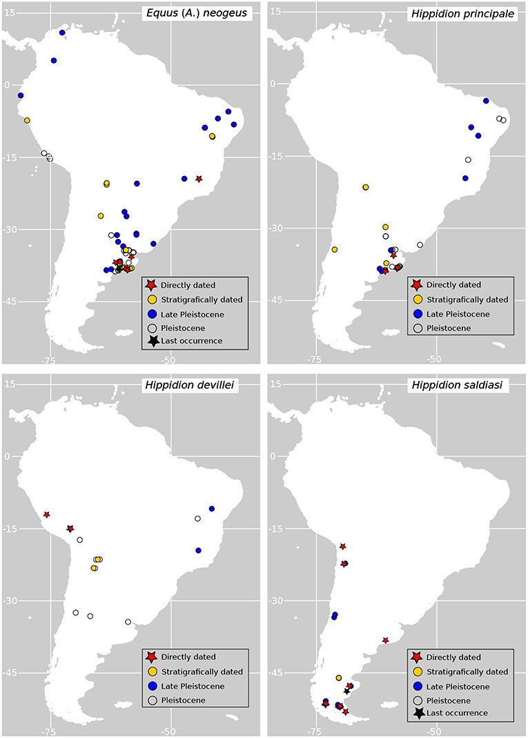
Figure 1. Geographic distribution of fossil records of horses used in this study. Directly dated records (red stars) are those corresponding to fossil specimens directly dated using radiocarbon dating; stratigraphically dated records (yellow dots) are those dated according to associated radiometric dates (i.e., ¹⁴C, ²³⁴U/²³⁰Th) on sediments or other stratigraphic features; Late Pleistocene (blue dots) and Pleistocene records (empty dots) are those fossil specimens which are tentatively assigned to the Pleistocene epoch or Late Pleistocene times according to the literature.

1.1. Horse Extinction in South America: Human vs. Environmental Drivers

Until now, what we know about the possible causes behind the extinction of horses in South America comes from regional analyses. In these studies (Prado et al., 2015; Barnosky et al., 2016; Villavicencio et al., 2016; Villavicencio and Werdelin, 2018) the radiocarbon chronology of megafaunal extinction is compared to the chronology of human presence and to the timing of major environmental changes in the areas under study, giving an idea of the possible role of the different factors in driving some of these extinctions. The most complete radiocarbon record for the presence and demise of Equus neogeus comes from the Pampas region of Argentina, Uruguay and Southern Brazil, and shows spatial coexistence between humans and horses for around 3,000 yr, dismissing a scenario of rapid overkill or “blitzkrieg” scenario [rapid extinction; Mosimann and Martin (1975)] in the area. At around 12 kyr BP (calendar years before present), E. neogeus disappears from the record, during a time of major vegetation changes in the Pampas (Prado et al., 2015; Barnosky et al., 2016). A similar situation is observed for the area of Última Esperanza in Southern Patagonia where the radiocarbon record for the presence of Hippidion saldiasi, the only horse inhabiting this region, shows at least 2,000 yr of spatial coexistence between humans and this species. This coexistence is followed by the disappearance of H. saldiasi from the record during a time of vegetation changes in the landscape from a grass steppe to Nothofagus forests (Villavicencio et al., 2016). A different situation is observed from a less robust chronology coming from the Andean Altiplano that records the existence in this area of Hippidion devillei during the late Pleistocene (Villavicencio and Werdelin, 2018). This record shows little evidence of temporal overlap between humans and horses in the area, with H. devillei disappearing from the record during a time of drying conditions. In summary, the chronology of horse disappearance in different regions shows no evidence of overkill of members of this group by human hunters, although it does not discard a more protracted role of humans in the process of extinction. At the same time, it shows a temporal coincidence of changes in the environment and the demise of horses, suggesting a possible important role for climatic changes in driving their extinction.

To explore the role of environmental changes in driving extinctions, we use paleo species distribution models (PSDM) to explore the dynamics of the climatic niche and the potential range of distribution of different species of horses as South America was transitioning from the Last Glacial Maximum (LGM) to the Holocene. Species distribution models have proven to be useful for determining the current distribution of common and rare species (Peterson et al., 2011; González-Salazar et al., 2013; Breiner et al., 2015), forecasting future distributions of species (Peterson et al., 2018; Raghavan et al., 2019), hindcasting the past distribution of extinct and extant species (Nogués-Bravo, 2009), predicting the yield of crops (Hannah et al., 2013; Raḿırez-Gil et al., 2018) among other applications. Niche modeling, and PSDM in particular, is a powerful tool for the study of the potential distribution (its spatial and temporal dynamics) of extinct horses in South America, which will allow us to assess the role of environmental changes in the extinction of South American horses.

2. Materials and Methods

Occurrence data of the species of Hippidion and Equus was compiled from the literature and the Paleobiology Database (https://paleobiodb.org/). The compilation consists of direct radiocarbon dates on different specimens as well as stratigraphically dated specimens. All the data was checked in the pertinent references and cleaned to avoid repetitions in the data. Only presences occurring from 21 kyr BP onwards and species with more than 5 records available were used to build the models. Even when species distribution models can be developed with a lower limit of three presences, we decided to be conservative and place a minimum of five occurrences to run the models (van Proosdij et al., 2016). Following these criteria, we were able to develop models for four taxa: Equus neogeus (26 presences), Hippidion principale (10 presences), Hippidion devillei (6 presences) and Hippidion saldiasi (23 presences). The geographic distribution of the fossil data used is presented in Figure 1 and Data Sheet 1, along with occurrences assigned tentatively to the late Pleistocene and the Pleistocene in the literature. Most of the occurrences used are assigned in the literature to the species level. Just three occurrences for Hippidion saldiasi are assigned to the species level with some uncertainty. This information is specified in the Data Sheet 1.

2.1. Climatic Layers

We generated downscaled (2.5 min) bioclimatic layers based on the layers from the software PaleoView (Fordham et al., 2017). We use average high and low monthly temperature and average monthly precipitation represented as a difference from present conditions, and for the period from 21 kyr BP to 8 kyr BP, between the latitudes of 15 degrees north to 60 degrees south, and between longitudes 87.5 degrees west to 27.5 degrees west. These layers were then used to apply the delta method modified to consider the changes in sea level (Schmatz et al., 2015). Past sea levels were estimated from previous publications (Fleming et al., 1998; Milne et al., 2005), coupled with the Gebco database for bathymetry and topography (Weatherall et al., 2015) and using the Worldclim 1.4 as current conditions for the delta method (Hijmans et al., 2005). We used Worldclim 1.4 instead of 2.0 since version 1.4 uses 1975 as reference to calculate differences in climate, the same as Paleoview and unlike Worldclim 2.0 (Fick and Hijmans, 2017). After generating the downscaled average high and low monthly temperature and average monthly precipitation, we used the biovars function from the dismo package (Hijmans et al., 2017) to generate the 19 biolcimatic variables usually used for Species Distribution Models. We used all the bioclimatic variables to build the species distribution models following (Phillips et al., 2006; Elith et al., 2011), using the regularization method to avoid overfitting (Allouche et al., 2006; Hastie et al., 2009; Merow et al., 2013). This method allows machine learning algorithm techniques to decide which biolclimatic variables are important to model the distribution of the different species analyzed. The variable selected for each of the species we used in this study can be found in the Supplementary Material section.

2.2. Modeling

The Maxnet package was used to model the distributions of all species (Phillips et al., 2004, 2017; Merow et al., 2013). For each species the bioclimatic conditions of the presences in each time slice plus the bioclimatic conditions of a thousand random background points were extracted. As mentioned above, only species with more than five presences were modeled. We used 5-fold cross validation to fit the models when they had more than 10 presences a three fold cross-validation if they had 10 or less presences. After the models were fit, True Skill Statistic (henceforth TSS) was used to select the threshold criteria (Allouche et al., 2006).

In order to get a confidence interval for the size of the geographic distribution, we used the TrinaryMaps package (Merow, 2019) to get high and low confidence interval on the threshold. This method detected the areas where the sensitivity is prioritized and thus detects most of the presences giving a larger distribution (Low confidence interval), and areas where the specificity is prioritized (High Confidence Interval) which means it will detect most of the false negatives resulting in a smaller range (Merow, 2019).

The predictive capacity of the models was evaluated using AUC (Area https://www.overleaf.com/3886381414dchghrxpdvrw Under the Curve) values obtained from the ROC curves (Fawcett, 2006).

3. Results

The predictive capacity of our models was high with values of AUC close to 0.9 (Table 1). The potential distributions for the four species analyzed here are presented as trinary maps (Figures 2–5, see section 2 Materials and Methods for more details) where blue represents areas of 0 probability of finding the species, white represents the potential distribution calculated using the low confidence interval (LCI, Table 1) of the threshold and red represents areas calculated from the high confidence interval (HCI, Table 1) of the threshold. These last are places with the highest probability of finding the species.

TABLE 1

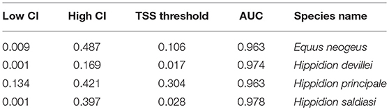
Table 1. Model evaluation parameters.

FIGURE 2

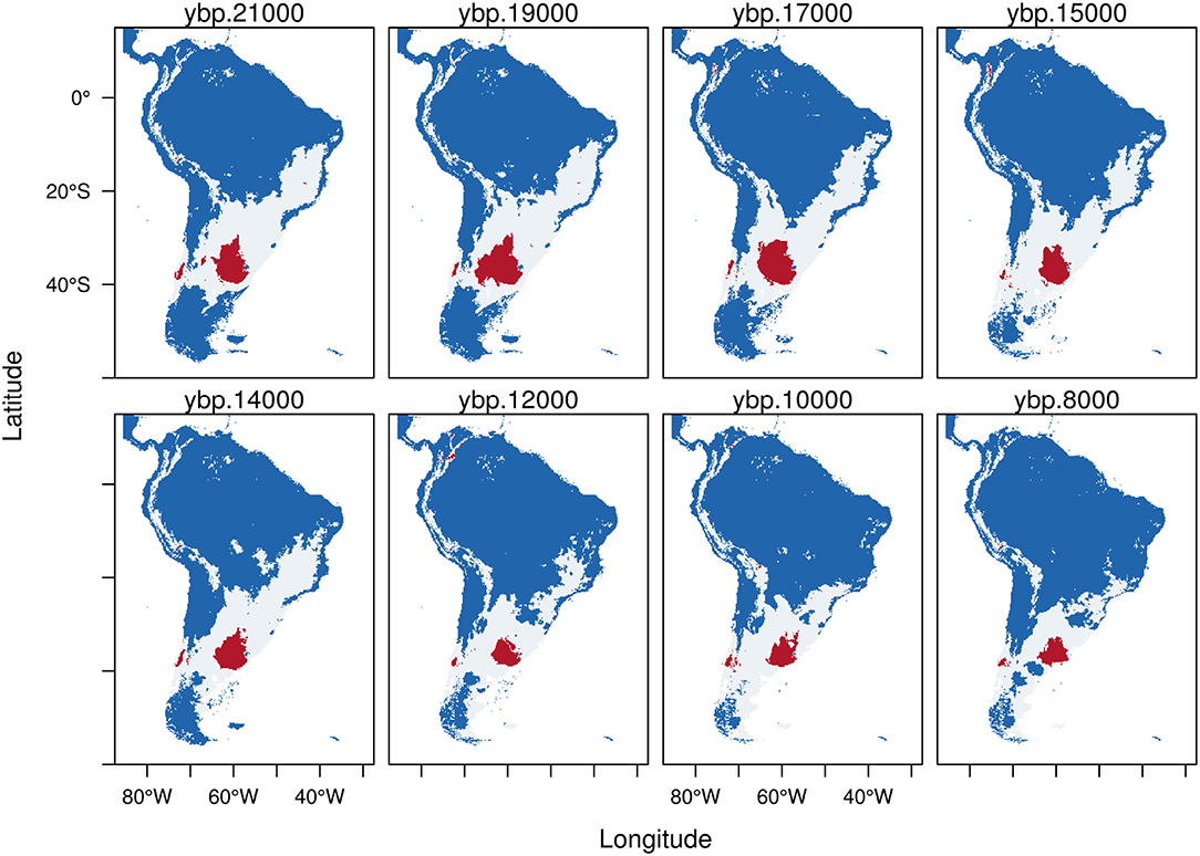
Figure 2. Trinary maps showing the potential distribution of Equus neogeus, calculated from the Last Glacial Maximum (LGM, 21 kyr BP) to the early Holocene (8 kyr BP). The different colors represent blue: areas where E. neogeus is not present; white: potential distribution of E. neogeus calculated from the low confidence interval of the threshold and red: potential distribution of E. neogeus calculated from the high confidence interval of the threshold. See methods for more details.

During the LGM (21 kyr BP), the predicted potential distribution of Equus neogeus (Figure 2) shows the highest probability of occurrence (red) in the Pampas region, central Chile and some very small patches in south-east Brazil and the northern Altiplano. The potential distribution estimated from the LCI (white area) shows a great potential extension of the area inhabited by E. neogeus covering from the Santa Cruz province in southern Argentina to the southern portion of north-east Brazil and forming a corridor to the west through central Chile. It is also present in the high Andes, going from the eastern Cordillera in Bolivia all the way north until the end of the Andean mountain range in Colombia. From the LGM through the early Holocene there is a reduction in both, areas calculated from the HCI (red) and the ones calculated from the LCI (white) of the potential distribution. Interesting is to notice that as the highly suitable areas of the Pampas became clearly reduced, the smaller one in central Chile persisted and some small patches became available in the Altiplano, eastern Bolivia and the northernmost portion of the Andean cordillera. At the same time, suitable environments suffer a southward shift during the early Holocene, reaching the southernmost portion of the continent in the Atlantic coast.

Hippidion principale exhibits a potential distribution mainly restricted to the southern cone during the LGM (Figure 3). The potential distribution estimated from HCI (red) goes from the Pampas extending south to the Santa Cruz province of Argentina. Hippidion principale also has an Andean distribution mostly situated in the high and western side of the Andes from north to south Chile. Further, between 17-15 kyr BP the model predicts the existence of a large pocket of potential area of distribution in the Amazon basin, which becomes an area of high probability of presence for H. principale. As we approach the transition to the Holocene, the potential distribution of H. principale becomes reduced and more displaced to the southern portion of the continent, as well as more fragmented. During the early Holocene, the remaining area of potential distribution estimated from the HCI (red) of the model calculations is located in the Pampas and extended to the adjacent western Andes. Some small portion remain in Southern Brazil and Southern Chile.

FIGURE 3

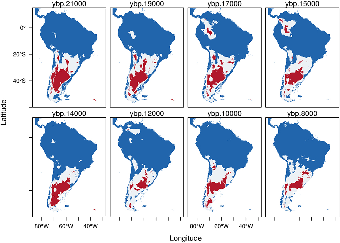
Figure 3. Trinary maps showing the potential distribution of Hippidion principale, calculated from the Last Glacial Maximum (LGM, 21 kyr BP) to the early Holocene (8 kyr BP). The different colors represent blue: areas where H. principale is not present; white: potential distribution of H. principale calculated from the low confidence interval of the threshold and red: potential distribution of H. principale calculated from the high confidence interval of the threshold. See methods for more details.

Hippidion devillei and H. saldiasi exhibit a small potential distribution during the time lapse analyzed, especially when we only consider the areas calculated from the HCI denoted in red (Figures 4, 5).

FIGURE 4

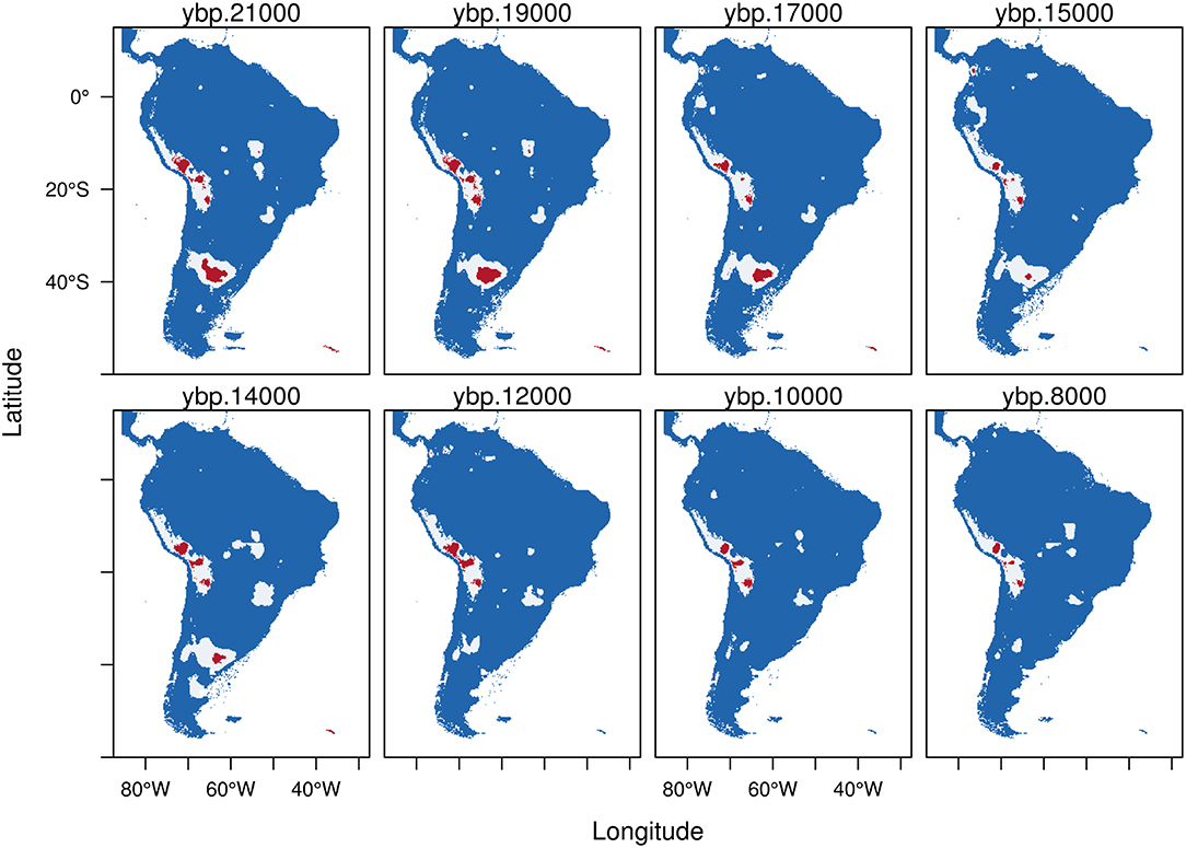
Figure 4. Trinary maps showing the potential distribution of Hippidion devillei, calculated from the Last Glacial Maximum (LGM, 21 kyr BP) to the early Holocene (8 kyr BP). The different colors represent blue: areas where H. devillei is not present; white: potential distribution of H. devillei calculated from the low confidence interval of the threshold and red: potential distribution of H. devillei calculated from the high confidence interval of the threshold. See methods for more details.

FIGURE 5

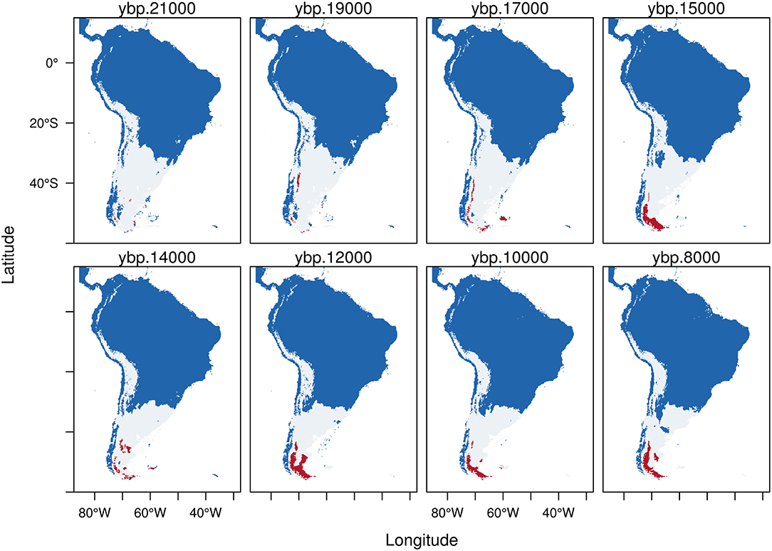
Figure 5. Trinary maps showing the potential distribution of Hippidion saldiasi, calculated from the Last Glacial Maximum (LGM, 21 kyr BP) to the early Holocene (8 kyr BP). The different colors represent blue: areas where H. saldiasi is not present; white: potential distribution of H. saldiasi calculated from the low confidence interval of the threshold and red: potential distribution of H. saldiasi calculated from the high confidence interval of the threshold. See methods for more details.

Hippidion devillei (Figure 4) during the LGM presents a fragmented distribution which includes a small portion of central Argentina and patches located in the Altiplano and central Peru. Some areas of the Amazon basin and south east Brazil are also assigned as places of potential distribution (red). All of these areas became reduced as we approach the Holocene and the last remnants that persist until 8 kyr BP are some patches in the Altiplano and in western Brazil.

Hippidion saldiasi (Figure 5) during the LGM has a potential distribution calculated from the LCI (white) located in the southern portion of the continent from Tierra del Fuego, covering all Argentina, central and northern Chile, and extending in the high Andes as far as northern Ecuador. There are very few areas of potential distribution estimated from the HCI during the LGM, which becomes bigger after about 16 kyr BP in southern Patagonia, reaching its highest extension between 13 and 11 kyr BP. While the rest of the potential area of distribution (white) becomes smaller as we approach the early Holocene, the areas of potential distribution estimated from the HCI (red) persist up to 8 kyr BP in the southern portion of the continent.

The dynamics of the potential area of distribution (in km²) calculated for the four different taxa using the TSS threshold through time is shown in Figure 6. Equus neogeus and Hippidion principale are the ones with the broadest distribution during the LGM with an estimated area close to 2.7 million km² for both of these taxa, while H. saldiasi potentially occupied an area of 1.4 million km² and H. devillei an area 7.9 thousand km². For all species there is a reduction in the potential areas of occupancy through time, and by 8 kyr BP Equus neogeus has lost a 61% of its potential area of distribution, H. principale a 36%, H. devillei a 55%, and H. saldiasi a 35%.

FIGURE 6

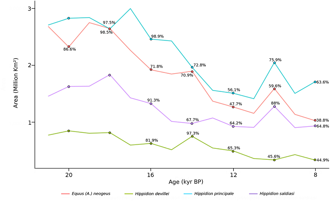
Figure 6. Estimated potential area (km²) of Equus (Amerhippus) neogeus, Hippidion principale, Hippidion devillei and Hippidion saldiasi, calculated from the LGM (21 kyr BP) to the early Holocene (8 kyr BP), every 1,000 yr interval. Percentage from the initial area calculated at 21 kyr are indicated at 20, 18, 16, 14, 12, 10, and 8 kyr BP. Percentages representing more area than the initial area omitted. This values are calculated from the TSS estimation. For the other values, see Data Sheet 2.

The diversity of horses at different times is shown in Figure 7. From the LGM to 14 kyr BP, it is possible to observe areas in central Argentina and the Pampas where the four species of horses potentially coexisted. The potential distribution of the four species together has its greatest extension at around 18 kyr BP. After 13 kyr BP, only a small area with a diversity of three species of horses is located in the southern portion of the Pampas, which remains until the end of our analyses at 8 kyr BP. By 10 kyr BP, new potential areas with a diversity of three species appear in the Altiplano and in portions of Southern Patagonia, disappearing by 8 kyr BP. An estimation of the change in biodiversity through time was calculated by subtracting the diversity at 8 kyr BP from the one calculated at 21 kyr BP (Δ Diversity in Figure 7). From this analysis we can see how the diversity is reduced in areas of central Argentina, the Pampas and Central Chile while increases in the southern portion of the continent and in some areas of the high Andes, north east Argentina and south east Brazil.

FIGURE 7

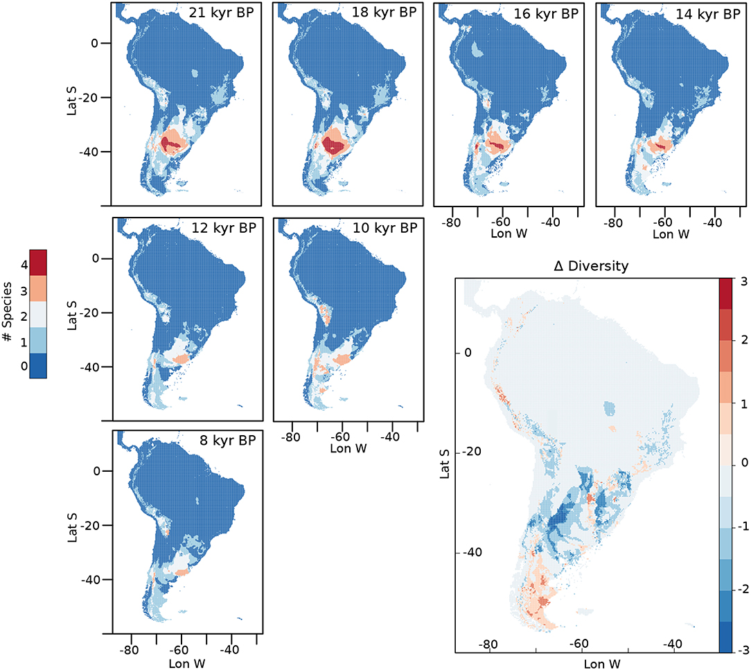
Figure 7. Diversity calculated for different moments from the LGM to 8 kyr BP. Delta diversity was calculated by subtracting the summed diversity at 8 kyr BP from the one calculated at 21 kyr BP.

4. Discussion

We have shown that the potential distribution of the analyzed species drastically decreased from the late Pleistocene through the Holocene and, according to the PSDM, no one was evidently driven to extinction due to changes in climate, suggesting that climate alone is not enough to explain the extinction of these taxa.

The PSDMs presented in this work correspond to presence only climatic models which use climatic information to establish the set of abiotic conditions that determine where the modeled species potentially could be present. Since only climatic variables are considered to model the potential distribution of these taxa, this model is suitable to assess the contribution of climate in affecting the potential distribution. But other contributing factors,associated to biotic interactions, for example, cannot be ruled out.

According to the above, what is being modeled by the PSDMs could be interpreted as the fundamental niche of the species; the set of abiotic conditions that determine the area where the species potentially could be present (Soberón and Peterson, 2005). In reality, however, at least two other major drivers can impact the distribution of a species, migration and biotic interactions (Soberón and Peterson, 2005). The idea that what is being modeled is the fundamental niche, instead of the realized niche, possibly leads to an overestimation of the potential area of distribution calculated by the models (Peterson et al., 2011). However, Varela et al. (2011) suggest that, due to the low number of presences commonly available to produce paleo species distribution models, it would be more common to underestimate the potential area of distribution of a species, due to the fact that fewer recorded occurrences imply a more sparse sampling of the conditions where the species was actually present according to the fossil record. Fortunately both potential biases compensate each other. However, further analyses with a larger dataset of species and of occurrences by species are required.

In order to take into account possible over estimation and under estimation of the potential areas of distribution calculated in this study we employ the trinary maps package (Merow, 2019). With the use of trinary maps, we were able to obtain scenarios where the sensitivity was prioritized (using the LCI of the threshold) which gave larger distributions, and scenarios where the specificity was prioritized (using the HCI of the threshold), which resulted in a smaller ranges. Having two scenarios is important in the case of study presented here, where taphonomic and preservation issues can introduce an important bias especially in the form of false negatives.

As it is expected in a scenario of global warming, like the one experienced during the transition from the LGM to the current interglacial, the potential distribution calculated for the late Pleistocene horses in South America became reduced in tropical and subtropical latitudes and persisted or shifted toward geographic areas where cooler conditions persisted longer. In this context, for example, the potential distribution of E. neogeus, which initially extended toward north-east Brazil, appears to be more shifted toward Patagonia and persistent in the high part of the Andes at 8 kyr BP (Figure 2). Hippidion devillei, which exhibits a small potential distribution during the LGM in the Pampas and the high Andes, persisted only in the last one at 8 kyr BP and disappeared from more tropical latitudes (Figure 4). Along this same line of argument, less evident are the changes observed for the distribution of H. principale and H. saldiasi as none of them experienced great shifts in the entire range of its potential distribution (Figures 3, 5). One main observation that can be drawn however, is that by the last time slice of our analysis only the areas located in the southernmost part of the calculated distributions and in the high Andes persisted.

Changes in diversity from the LGM to the early Holocene show a significant reduction in biodiversity in subtropical and tropical areas and an increase in Patagonia and some high Andean places, which also reflects a preference toward the areas of the continent where cooler conditions persisted longer (Figure 7, Δ Diversity).

It is important to acknowledge that the displacement and the changes in size of the potential distribution of horses could be related to more variables than just temperature (see Supplementary Material). In this sense, vegetation changes that were happening all over the continent during the Pleistocene Holocene transition could have had an important role in driving some of the changes in distribution observed in this study. These vegetation re-configurations, in turn, are ultimately related to changes in precipitation and temperature patterns.

4.1. Potential Distribution and Ecological Preferences of South American Horses

The potential distribution calculated for Equus neogeus during the LGM included areas with grassland steppe and temperate semi-deserts in the Pampas and more tropical savanna environments in east Brazil, as some environmental reconstructions suggest for this time (Ray and Adams, 2001; de Melo França et al., 2015). This observation does not contradict what is known about the diet and the environments inhabited by E. neogeus derived from stable isotopes studies, which suggest the occupancy and consumption of plants from the entire spectrum of C3 plants, C4 plants, and mixed C3-C4 diet (Prado and Alberdi, 2017 and references there). Hippidion principale would have occupied areas of grasslands and temperate deserts according to the potential distribution calculated by our models and the vegetation reconstructions for the continent during the LGM (Ray and Adams, 2001; de Melo França et al., 2015). In the case of H. devillei and H. saldiasi, their potential distribution indicates they occupied areas with temperate deserts and semi-deserts during the LGM, as well as colder areas in the high Andes and in the southern tip of the continent (Ray and Adams, 2001; de Melo França et al., 2015). This agrees with the results from stable isotope analyses showing that all species in the genus Hippidion during the Pleistocene preferred woodlands or C3 wooded open areas, with a diet of C3 plants or C4-C3 mixed [Prado and Alberdi (2017) and references there].

The area with the highest diversity of horses during the LGM is the Pampas (Figure 7). End Pleistocene Pampas was a C3- dominated grassland steppe, representing a sub-humid and arid environment which changed, starting at 12 kyr BP, to a major proportion of C4 vegetation, as the climate became more humid and warmer (Prieto, 1996; Iriarte, 2006; Suárez, 2011). These changes would have been negative for the species of Hippidion in the area given their habitat preferences discussed above. Accordingly, the timing of changes in vegetation coincides with a major reduction in the potential distribution of Hippidion principale between 13 and 12 kyr BP in the area (Figure 3) and with the timing of a drop in biodiversity in the area from four to three species of horses at around 12 kyr BP (Figure 7).

4.2. Area of Potential Distribution: Body Size and Extinction Risk

It is interesting to notice that the species of horses with the greater calculated area of occupancy (Figure 6) are the ones with greater body size. Hippidion principale, with an estimated body size of 460 kg (Alberdi et al., 1995) and Equus neogeus with a body size of 370 kg (Prado and Alberdi, 1994) had a potential area of distribution of around 2.7 million km². On the other hand, the smallest species Hippidion devillei (250 kg, Alberdi et al., 1995), has the most reduced potential area of distribution with an estimate of around 793 thousand km² during the LGM. Hippidion saldiasi, with an estimated body size of 265 kg (Alberdi et al., 1995), has a potential area of occupancy of 1.4 million km².

All taxa of horses analyzed here experienced a significant reduction in the area of potential occupation according to the information in Figure 6. E. neogeus experienced the greatest reduction losing 61% of its distribution from the LGM to 8 kyr BP. According to the radiocarbon chronology for this taxon, it disappears from the record of South America at around 11.7 kyr BP (Rio Quequen Salado, Argentina, Prado et al., 2015), a time that coincides with a reduction of its potential area of distribution by half. This last appearance date (black star, Figure 1) is located in the area calculated for the distribution of Equus neogeus at 12 kyr BP (red, Figure 2). Something slightly different is observed for H. saldiasi. The greatest reduction of the potential area of distribution for this taxon occurs at 9 kyr BP and corresponds to a loss of a 37% of the area calculated. This result could suggest that the potential area of distribution of H. saldiasi was less affected by the climatic changes of the late glacial and early Holocene when compared to E. neogeus, for example. Interestingly, the radiocarbon record for H. saldiasi shows the last appearance date close to 10 kyr BP (Cerro Bombero, Argentina, Paunero et al., 2008), being the last horse species becoming extinct in the continent according to the information available at the moment.

Hippidion devillei and H. principale had the greatest reduction in their potential distribution at 11 kyr BP, with a reduction of 51% and 47%, respectively. The radiocarbon record for these two taxa shows last appearance dates of 12.8 kyr BP and 15.3 kyr BP, respectively, however, it is still scarce in terms of the total number of dates to make conclusions about the timing of extinction of these horses.

A deeper analysis about the impact that a reduction in the potential area of occupancy from the LGM to the early Holocene was performed.To begin with, we calculated the minimum area needed to have a population of horses that could persist in time and compare that calculation with the potential areas of occupancy estimated from the PSDM (Figure 6). We used the following information: there is evidence that for mammals, the number of individuals that can inhabit in a certain area is affected by body size (Marquet and Taper, 1998) and that the minimum viable population for ungulates in natural conditions is 4,354 individuals (calculated using the information and methods provided in Traill et al., 2007). We used the estimations for body size available in the literature (first paragraph, section 4.2) to determine the home range needed for each of the different species of horses knowing that home range scales positively with body size (Lindstedt et al., 1986). Following the work carried out by Marquet and Taper (1998) on body size and extinction risk of mammalian species in islands, we then multiplied these home range values by the minimum viable population size (4,354 individuals) to finally calculate the minimum viable area (MVA) for each taxon. The results of these calculations are in Table 2. From the values presented there and the ones from Figure 6 we can conclude that by 8 kyr BP E. neogeus has an estimated area of occupancy 20.3 times larger that its MVA, H. devillei 9.5 times its MVA, H. principale close to 29.4 times its MVA, and H. saldiasi 31.8 times it MVA. A more conservative approach was to calculate MVAs using only the potential areas of distribution calculated from the high confidence interval from the trinary maps, which in turn results in smaller potential areas. Also, we left out every contiguous patch of area that was smaller than the calculated MVA for the different species. As a result, by 8 kyr BP, E. neogeus has an occupancy area 6.18 times its MVA, H. devillei one 1.08 times its MVA, H. principale an area 15.1 times its MVA, and H. saldiasi an estimated area of occupancy 6.83 times the MVA needed for its survival. This conservative scenario leaves H. devillei as the only species under a very high risk of extinction under these conditions. In summary, all these calculations suggest that the inferred climate-driven changes in the potential distribution of horses are not sufficient to explain the extinction of these taxa at the end of the Pleistocene in South America, thus other causes to explain their extinction should be invoked.

TABLE 2

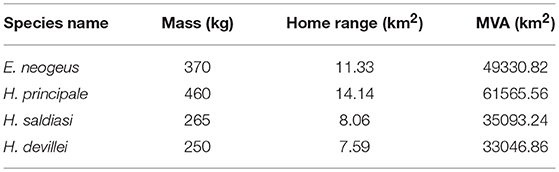
Table 2. Minimum Viable Area (MVA).

In Figure 8 is shown the distribution of radiocarbon dates on archaeological sites from the time of human arrival into South America at around 16 kyr (Monte Verde, Chile, in Dillehay, 1997) to the early Holocene. As shown in this figure, from the time of colonization, there is a constant increase in the estimated number of sites and radiocarbon dates recording the presence of people in the continent. At the same time, from the time interval between 13 and 12 kyr BP, the presence of humans is evident in most of the regions in the continent, which could have led to an increase in human impacts in the main different ecosystems of South America. Some of these ecosystems may have been particularly more vulnerable to human impacts as well (Pires et al., 2015). Comparing these observations with the changes in the potential distribution of horses we can see, for example, that reductions close to a 50% of the potential area occupied by E. neogeus and H. principale happened around 13 kyr BP, a time when humans where already present in almost every environment (Figure 8). The major increase in the number of sites with evidence of humans is recorded between 10-9 kyr BP, time at which all the horse species studied had already experienced a major reduction in their potential distribution.

FIGURE 8

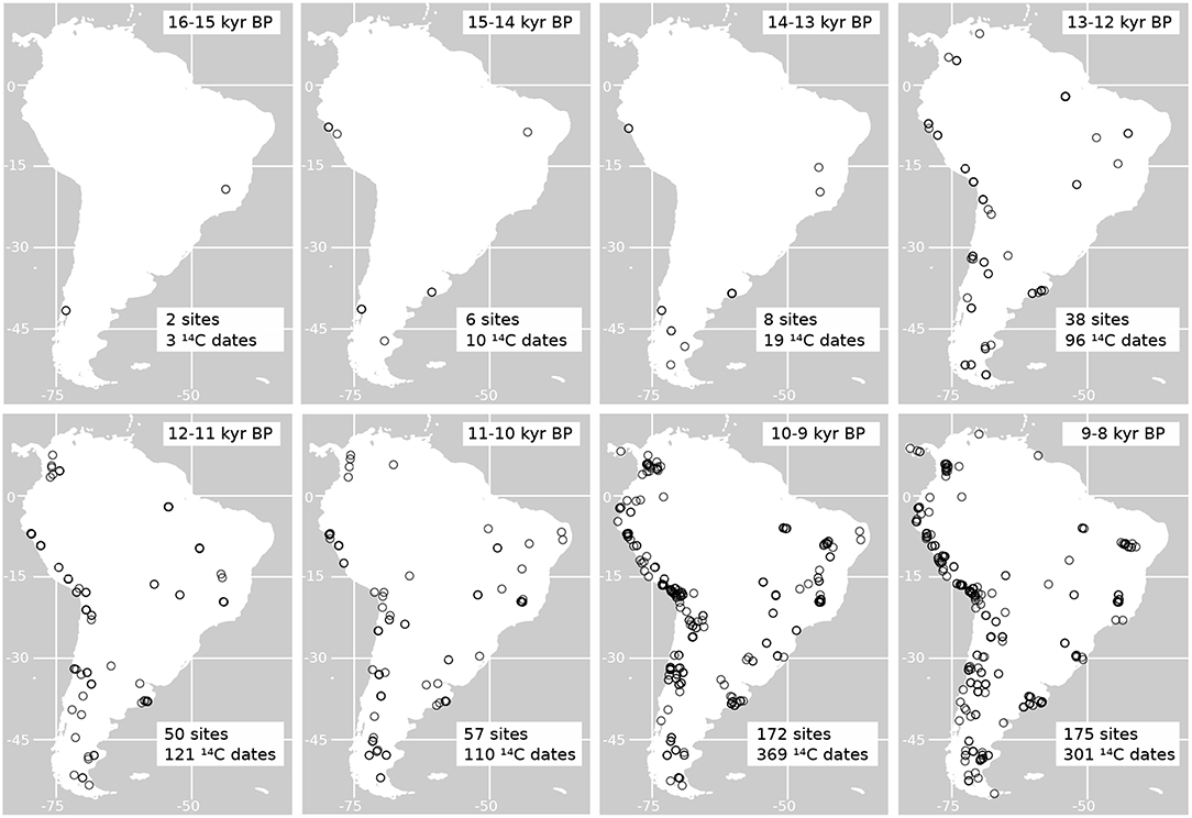
Figure 8. Maps of the geographic distribution of radiocarbon dates on archaeological sites indicating the presence of humans in South America. The number of archaeological sites and radiocarbon dates graphed per time bin are indicated in each map. All dates were calibrated using Calib 7.02 and the calibration curve SH13 (Hogg et al., 2013). Dates where obtained from the databases published by Gayo et al. (2015) and Goldberg et al. (2016).

5. Conclusions

According to the models presented here, there is an evident reduction in the potential distribution of the four species of horses from the LGM to 8 kyr BP in South America. In general, the reduction in the size of the areas of potential distribution is accompanied by a shift in the location of the estimated distribution toward southern latitudes and higher altitudes where cooler conditions persisted longer compared to tropical and subtropical latitudes. The changes in diversity of horses follow the same pattern of shifts toward areas of cooler conditions at the beginning of the Holocene, experiencing a decrease in the number of horse taxa in tropical and subtropical latitudes and an increase in the number of species in the high Andes and Patagonia when we compare the LGM diversity with the one calculated at 8 kyr BP.

It is possible to suggest an increasing extinction risk through time for the species of horses studied as we noticed major reductions, between a 50% and 37%, of the potential area of distribution when we compared the LGM to the time slice at 8 kyr BP.

An important statement to make is that, even if there are major reductions in the potential areas of distribution from the LGM toward the early Holocene according to the PSDM, these do not reach levels indicating high extinction risks, suggesting that climate change, alone, is not able to explain the extinction of late Pleistocene horses in South America but for one species (Hippidion devillei). In this line of argument is important to recall that the reductions in area happened at times when humans where already present in most of the environments of the continent with increasing presence (and maybe impacts) in the landscape. This opens once more the possibility of synergistic effects between humans and environmental changes in driving some of the late Quaternary extinctions in South America.

Data Availability

The datasets for this study can be found in the Supplementary Material.

Author Contributions

NV: conceived original idea, data gathering, data analysis, discussion, and manuscript preparation. DC: data gathering, data analysis, discussion, and manuscript preparation. PM: data analysis, discussion, and manuscript preparation.

Conflict of Interest Statement

The authors declare that the research was conducted in the absence of any commercial or financial relationships that could be construed as a potential conflict of interest.

Acknowledgments

We thank our funding sources: Postdoctoral fellowship Fondecyt 3170706, IEB AFB17008 and the SPARC project GEF-5810. We also thank the two reviewers, Dr. Dimila Mothé and Dr. Tiago Simoes, for their insightful comments that helped us to improve this manuscript.

Supplementary Material

The Supplementary Material for this article can be found online at: https://www.frontiersin.org/articles/10.3389/fevo.2019.00226/full#supplementary-material

References

Alberdi, M. T., and Frassinetti, D. (2000). Presencia de Hippidion y Equus (Amerhippus) (Mammalia, Perissodactyla) y su distribución en el Pleistoceno superior de Chile. Estud. Geol. 56, 279–290. doi: 10.3989/egeol.00565-6144

CrossRef Full Text | Google Scholar

Alberdi, M. T., and Prado, J. L. (2004). Caballos Fósiles de América del Sur. Madrid: INCUAPA, I. Departamento de Paleobiología, Museo Nacional de Ciencias Naturales, CSIC. José Gutiérrez Abascal.

Google Scholar

Alberdi, M. T., Prado, J. L., and Ortiz-Jaureguizar, E. (1995). Patterns of body size changes in fossil and living Equini (perissodactyla). Biol. J. Linn. Soc. 54, 349–370. doi: 10.1111/j.1095-8312.1995.tb01042.x

CrossRef Full Text | Google Scholar

Allouche, O., Tsoar, A., and Kadmon, R. (2006). Assessing the accuracy of species distribution models: prevalence, kappa and the true skill statistic (tss). J. Appl. Ecol. 43, 1223–1232. doi: 10.1111/j.1365-2664.2006.01214.x

CrossRef Full Text | Google Scholar

Barnosky, A. D., Lindsey, E. L., Villavicencio, N. A., Bostelmann, E., Hadly, E. A., Wanket, J., et al. (2016). Variable impact of late-quaternary megafaunal extinction in causing ecological state shifts in north and south america. Proc. Natl. Acad. Sci. U.S.A. 113, 856–861. doi: 10.1073/pnas.1505295112

PubMed Abstract | CrossRef Full Text | Google Scholar

Breiner, F. T., Guisan, A., Bergamini, A., and Nobis, M. P. (2015). Overcoming limitations of modelling rare species by using ensembles of small models. Methods Ecol. Evol. 6, 1210–1218. doi: 10.1111/2041-210X.12403

CrossRef Full Text | Google Scholar

Brook, B. W., and Barnosky, A. D. (2012). “Quaternary extinctions and their link to climate change,” in Saving a Million Species, ed L. Hannah (Washington, DC: Springer), 179–198.

Google Scholar

de Melo França, L., de Asevedo, L., Dantas, M. A. T., Bocchiglieri, A., dos Santos Avilla, L., Lopes, R. P., et al. (2015). Review of feeding ecology data of late pleistocene mammalian herbivores from south america and discussions on niche differentiation. Earth Sci. Rev. 140, 158–165. doi: 10.1016/j.earscirev.2014.10.006

CrossRef Full Text | Google Scholar

Dillehay, T. D. (1997). Monte Verde, a Late Pleistocene Settlement in Chile: The Archaeological Context and Interpretation, Vol. 2. Washington, DC: Smithsonian Inst Press.

Google Scholar

Eisenmann, V. (1979). Les métapodes d'equus sensu lato (mammalia, perissodactyla). Geobios 12, 863–886. doi: 10.1016/S0016-6995(79)80004-2

CrossRef Full Text | Google Scholar

Elith, J., Phillips, S. J., Hastie, T., Dudík, M., Chee, Y. E., and Yates, C. J. (2011). A statistical explanation of maxent for ecologists. Divers. Distribut. 17, 43–57. doi: 10.1111/j.1472-4642.2010.00725.x

CrossRef Full Text | Google Scholar

Fawcett, T. (2006). An introduction to roc analysis. Patt. Recogn. Lett. 27, 861–874. doi: 10.1016/j.patrec.2005.10.010

CrossRef Full Text | Google Scholar

Fick, S. E., and Hijmans, R. J. (2017). Worldclim 2: new 1-km spatial resolution climate surfaces for global land areas. Int. J. Climatol. 37, 4302–4315. doi: 10.1002/joc.5086

CrossRef Full Text | Google Scholar

Fleming, K., Johnston, P., Zwartz, D., Yokoyama, Y., Lambeck, K., and Chappell, J. (1998). Refining the eustatic sea-level curve since the last glacial maximum using far-and intermediate-field sites. Earth Planet. Sci. Lett. 163, 327–342. doi: 10.1016/S0012-821X(98)00198-8

CrossRef Full Text | Google Scholar

Fordham, D. A., Saltré, F., Haythorne, S., Wigley, T. M., Otto-Bliesner, B. L., Chan, K. C., et al. (2017). Paleoview: a tool for generating continuous climate projections spanning the last 21 000 years at regional and global scales. Ecography 40, 1348–1358. doi: 10.1111/ecog.03031

CrossRef Full Text | Google Scholar

Gayo, E. M., Latorre, C., and Santoro, C. M. (2015). Timing of occupation and regional settlement patterns revealed by time-series analyses of an archaeological radiocarbon database for the south-central andes (16–25 s). Q. Int. 356, 4–14. doi: 10.1016/j.quaint.2014.09.076

CrossRef Full Text | Google Scholar

Goldberg, A., Mychajliw, A. M., and Hadly, E. A. (2016). Post-invasion demography of prehistoric humans in south america. Nature 532:232. doi: 10.1038/nature17176

PubMed Abstract | CrossRef Full Text | Google Scholar

González-Salazar, C., Stephens, C. R., and Marquet, P. A. (2013). Comparing the relative contributions of biotic and abiotic factors as mediators of species distributions. Ecol. Model. 248, 57–70. doi: 10.1016/j.ecolmodel.2012.10.007

CrossRef Full Text | Google Scholar

Hannah, L., Roehrdanz, P. R., Ikegami, M., Shepard, A. V., Shaw, M. R., Tabor, G., et al. (2013). Climate change, wine, and conservation. Proc. Natl. Acad. Sci. U.S.A. 110, 6907–6912. doi: 10.1073/pnas.1210127110

PubMed Abstract | CrossRef Full Text | Google Scholar

Hastie, T., Tibshirani, R., and Friedman, J. (2009). The Elements of Statistical Learning: Data Mining, Inference, and Prediction. New York, NY: Springer Series in Statistics. doi: 10.1007/978-0-387-84858-7

CrossRef Full Text | Google Scholar

Hijmans, R. J., Cameron, S. E., Parra, J. L., Jones, P. G., and Jarvis, A. (2005). Very high resolution interpolated climate surfaces for global land areas. Int. J. Climatol. 25, 1965–1978. doi: 10.1002/joc.1276

CrossRef Full Text | Google Scholar

Hijmans, R. J., Phillips, S., Leathwick, J., and Elith, J. (2017). dismo: Species Distribution Modeling. R package version 1.1-4.

Google Scholar

Hoffstetter, R. (1950). Algunas observaciones sobre los caballos fósiles de américa del sur. amerhippus gen. nov. Boletín Informaciones Científicas Nacionales 3, 426–454.

Google Scholar

Hogg, A. G., Hua, Q., Blackwell, P. G., Niu, M., Buck, C. E., Guilderson, T. P., et al. (2013). Shcal13 southern hemisphere calibration, 0–50,000 years cal bp. Radiocarbon 55, 1889–1903. doi: 10.2458/azu_js_rc.55.16783

CrossRef Full Text | Google Scholar

Iriarte, J. (2006). Vegetation and climate change since 14,810 14 c yr bp in southeastern uruguay and implications for the rise of early formative societies. Q. Res. 65, 20–32. doi: 10.1016/j.yqres.2005.05.005

CrossRef Full Text | Google Scholar

Koch, P. L., and Barnosky, A. D. (2006). Late quaternary extinctions: state of the debate. Annu. Rev. Ecol. Evol. Systemat. 37, 215–250. doi: 10.1146/annurev.ecolsys.34.011802.132415

CrossRef Full Text | Google Scholar

Lindstedt, S. L., Miller, B. J., and Buskirk, S. W. (1986). Home range, time, and body size in mammals. Ecology 67, 413–418. doi: 10.2307/1938584

CrossRef Full Text | Google Scholar

Machado, H., Grillo, O., Scott, E., and Avilla, L. (2018). Following the footsteps of the south american equus: are autopodia taxonomically informative? J. Mamm. Evol. 25, 397–405. doi: 10.1007/s10914-017-9389-6

CrossRef Full Text | Google Scholar

Marquet, P. A., and Taper, M. L. (1998). On size and area: patterns of mammalian body size extremes across landmasses. Evol. Ecol. 12, 127–139. doi: 10.1023/A:1006567227154

CrossRef Full Text | Google Scholar

Merow, C. (2019). Build Trinary (Not Binary) Maps That Show Upper and Lower Bounds on Species' Ranges. Available online at: https://github.com/cmerow/trinaryMaps

Google Scholar

Merow, C., Smith, M. J., and Silander, J. A. Jr. (2013). A practical guide to maxent for modeling species distributions: what it does, and why inputs and settings matter. Ecography 36, 1058–1069. doi: 10.1111/j.1600-0587.2013.07872.x

CrossRef Full Text | Google Scholar

Milne, G. A., Long, A. J., and Bassett, S. E. (2005). Modelling holocene relative sea-level observations from the caribbean and south america. Q. Sci. Rev. 24, 1183–1202. doi: 10.1016/j.quascirev.2004.10.005

CrossRef Full Text | Google Scholar

Mosimann, J. E., and Martin, P. S. (1975). Simulating overkill by paleoindians: did man hunt the giant mammals of the new world to extinction? mathematical models show that the hypothesis is feasible. Am. Sci. 63, 304–313.

Google Scholar

Nogués-Bravo, D. (2009). Predicting the past distribution of species climatic niches. Glob. Ecol. Biogeogr. 18, 521–531. doi: 10.1111/j.1466-8238.2009.00476.x

CrossRef Full Text | Google Scholar

Orlando, L., Male, D., Alberdi, M. T., Prado, J. L., Prieto, A., Cooper, A., and Hänni, C. (2008). Ancient dna clarifies the evolutionary history of american late pleistocene equids. J. Mol. Evol. 66, 533–538. doi: 10.1007/s00239-008-9100-x

PubMed Abstract | CrossRef Full Text | Google Scholar

Paunero, R. S., Rosales, G., Prado, J. L., and Alberdi, M. T. (2008). Cerro bombero: registro de hippidion saldiasi roth, 1899 (equidae, perissodactyla) en el holoceno temprano de patagonia (santa cruz, argentina). Estud. Geol. 64, 89–98. doi: 10.3989/egeol.08641430

CrossRef Full Text | Google Scholar

Peterson, A. T., Cobos, M. E., and Jiménez-García, D. (2018). Major challenges for correlational ecological niche model projections to future climate conditions. Ann. N. Y. Acad. Sci. 1429, 66–77. doi: 10.1111/nyas.13873

PubMed Abstract | CrossRef Full Text | Google Scholar

Peterson, A. T., Soberón, J., Pearson, R. G., Anderson, R. P., Martínez-Meyer, E., Nakamura, M., et al. (2011). Ecological Niches and Geographic Distributions (MPB-49), Vol. 56. Woodstock, UK: Princeton University Press. doi: 10.23943/princeton/9780691136868.001.0001

CrossRef Full Text | Google Scholar

Phillips, S. J., Anderson, R. P., Dudík, M., Schapire, R. E., and Blair, M. E. (2017). Opening the black box: an open-source release of maxent. Ecography 40, 887–893. doi: 10.1111/ecog.03049

CrossRef Full Text | Google Scholar

Phillips, S. J., Anderson, R. P., and Schapire, R. E. (2006). Maximum entropy modeling of species geographic distributions. Ecol. Model. 190, 231–259. doi: 10.1016/j.ecolmodel.2005.03.026

CrossRef Full Text | Google Scholar

Phillips, S. J., Dudík, M., and Schapire, R. E. (2004). “A maximum entropy approach to species distribution modeling,” in Proceedings of the Twenty-First International Conference on Machine Learning (Banff, AB: ACM), 83–90.

Google Scholar

Pires, M. M., Koch, P. L., Fariña, R. A., de Aguiar, M. A., dos Reis, S. F., and Guimarães, P. R. (2015). Pleistocene megafaunal interaction networks became more vulnerable after human arrival. Proc. R. Soc. B 282:20151367. doi: 10.1098/rspb.2015.1367

PubMed Abstract | CrossRef Full Text | Google Scholar

Prado, J. L., and Alberdi, M. T. (1994). A quantitative review of the horse Equus from South America. Palentology 37, 459–481.

Google Scholar

Prado, J. L., and Alberdi, M. T. (2017). Fossil Horses of South America. Phylogeny, Systemics and Ecology. Cham: Springer.

PubMed Abstract | Google Scholar

Prado, J. L., Martinez-Maza, C., and Alberdi, M. T. (2015). Megafauna extinction in south america: a new chronology for the argentine pampas. Palaeogeogr. Palaeoclimatol. Palaeoecol. 425, 41–49. doi: 10.1016/j.palaeo.2015.02.026

CrossRef Full Text | Google Scholar

Prieto, A. R. (1996). Late quaternary vegetational and climatic changes in the pampa grassland of argentina. Quat. Res. 45, 73–88. doi: 10.1006/qres.1996.0007

CrossRef Full Text | Google Scholar

Raghavan, R. K., Peterson, A. T., Cobos, M. E., Ganta, R., and Foley, D. (2019). Current and future distribution of the lone star tick, amblyomma americanum (l.) (acari: Ixodidae) in north america. PLoS ONE 14:e0209082. doi: 10.1371/journal.pone.0209082

PubMed Abstract | CrossRef Full Text | Google Scholar

Ramírez-Gil, J. G., Morales, J. G., and Peterson, A. T. (2018). Potential geography and productivity of hass avocado crops in colombia estimated by ecological niche modeling. Sci. Horticult. 237, 287–295. doi: 10.1016/j.scienta.2018.04.021

CrossRef Full Text | Google Scholar

Ray, N., and Adams, J. (2001). A gis-based vegetation map of the world at the last glacial maximum (25,000-15,000 bp). Int. Archaeol. 11. doi: 10.11141/ia.11.2

CrossRef Full Text | Google Scholar

Schmatz, D., Luterbacher, J., Zimmermann, N., and Pearman, P. (2015). Gridded climate data from 5 gcms of the last glacial maximum downscaled to 30 arc s for europe. Clim. Past Discuss. 11, 2585–2613. doi: 10.5194/cpd-11-2585-2015

CrossRef Full Text | Google Scholar

Soberón, J., and Peterson, A. T. (2005). Interpretation of models of fundamental ecological niches and species distributional area. Biodivers. Informat. 2, 1–10. doi: 10.17161/bi.v2i0.4

CrossRef Full Text | Google Scholar

Suárez, R. (2011). Arqueología Durante la Transicio Pleistoceno Holoceno: Componentes Paleoindios, Organizacion de la Tecnología y Movilidad de Los Primeros Americanos en Uruguay. Oxford: British Archaeological Reports.

Google Scholar

Traill, L. W., Bradshaw, C. J., and Brook, B. W. (2007). Minimum viable population size: a meta-analysis of 30 years of published estimates. Biol. Conserv. 139, 159–166. doi: 10.1016/j.biocon.2007.06.011

CrossRef Full Text | Google Scholar

van Proosdij, A. S., Sosef, M. S., Wieringa, J. J., and Raes, N. (2016). Minimum required number of specimen records to develop accurate species distribution models. Ecography 39, 542–552. doi: 10.1111/ecog.01509

CrossRef Full Text | Google Scholar

Varela, S., Lobo, J. M., and Hortal, J. (2011). Using species distribution models in paleobiogeography: a matter of data, predictors and concepts. Palaeogeogr. Palaeoclimatol. Palaeoecol. 310, 451–463. doi: 10.1016/j.palaeo.2011.07.021

CrossRef Full Text | Google Scholar

Villavicencio, N. A., Lindsey, E. L., Martin, F. M., Borrero, L. A., Moreno, P. I., Marshall, C. R., et al. (2016). Combination of humans, climate, and vegetation change triggered late quaternary megafauna extinction in the última esperanza region, southern patagonia, chile. Ecography 39, 125–140. doi: 10.1111/ecog.01606

CrossRef Full Text | Google Scholar

Villavicencio, N. A., and Werdelin, L. (2018). The casa del diablo cave (puno, peru) and the late pleistocene demise of megafauna in the andean altiplano. Q. Sci. Rev. 195, 21–31. doi: 10.1016/j.quascirev.2018.07.013

CrossRef Full Text | Google Scholar

Weatherall, P., Marks, K. M., Jakobsson, M., Schmitt, T., Tani, S., Arndt, J. E., et al. (2015). A new digital bathymetric model of the world's oceans. Earth Space Sci. 2, 331–345. doi: 10.1002/2015EA000107

CrossRef Full Text | Google Scholar