Network-Based Biomonitoring: Exploring Freshwater Food Webs With Stable Isotope Analysis and DNA Metabarcoding

Introduction

Freshwater ecosystems, which house a disproportionate amount of Earth's biodiversity (Dudgeon et al., 2006), face multiple threats (Cazzolla Gatti, 2016; Hu et al., 2017). Freshwater availability (Rodell et al., 2018) and habitat extent (e.g., Dixon et al., 2016) are in decline in most parts of the world. Yet, the very structural and ecological complexity that gives freshwater systems their capacity for biodiversity and ecosystem services also makes them very difficult to study. This is particularly true for the planet's wetlands, which are generally viewed as hard to define, seasonally variable, and often inaccessible.

While widely studied by ecologists, food web networks are under-utilized in bioassessment, even though they provide a wide range of information–from taxon-specific, node-to-node information to higher order information aggregated across the community–and are a tool for visualizing the dense information in complex systems, such as wetlands. Metrics from food web analysis can be used to infer their stability (May, 1972), robustness to biodiversity loss (Estrada, 2007; Gilbert, 2009), and different assembly or interaction mechanisms (Vázquez, 2005; Williams, 2011). Food web networks explicitly show biodiversity, species interactions, and structural and functional relationships of ecosystems (Dunne et al., 2002b; Thompson et al., 2012), and are an intuitive communication tool for environmental managers, particularly when presenting to lay audiences. However, constructing food webs is laborious (Thompson et al., 2012), underscoring the need for new tools that can facilitate this process to support wider implementation in bioassessment (Bohan et al., 2017).

DNA metabarcoding has the potential to revolutionize biomonitoring and bioassessment by providing a fast way of consistently observing biodiversity in high-resolution detail (Baird and Hajibabaei, 2012). Further, DNA metabarcoding can be both more cost-effective and more efficient than traditional biomonitoring (Aylagas et al., 2018). The rapid adoption of DNA metabarcoding can be seen in the exponential rise in the number of papers published about biomonitoring with DNA metabarcoding in the last decade¹. While much of the early literature focused on assessing how well DNA metabarcoding technologies could reproduce biodiversity data collected by traditional means (e.g., Gibson et al., 2015; Emilson et al., 2017), more recent efforts have expanded the application of this approach, exploring possibilities for leveraging genomic data in novel ways (e.g., Gray et al., 2014; Bohan et al., 2017; Derocles et al., 2018; Deagle et al., 2019).

Concurrently, efforts have sought to make use of organism traits to leverage existing biodiversity knowledge for bioassessment. Traits-based approaches assume that environmental filtering selects species with suites of traits that allow them to coexist under similar environmental conditions (Poff, 1997). Since many species share the same traits, traits-based approaches are taxon-free measures of biodiversity (sensu Damuth et al., 1992; Doledec and Statzner, 2008; Andrews and Hixson, 2014). Body size, for example, is a trait that aggregates information across taxonomic groups, and has been invoked as a powerful, trait-based indicator of community responses to disturbance (Liu et al., 2015). While growing interest in traits-based approaches has prompted some of its key advocates to call it a “bandwagon” (McGill, 2015; Didham et al., 2016), we argue trait-based approaches have failed to realize their full potential, focusing primarily upon phenomenological case studies and relying on re-application of traits approaches to traditional analyses (e.g., ordination approaches). This approach has led to vacuous generalizations about traits approaches, lacking in mechanistic evidence (Didham et al., 2016). Recently there has been growing interest in using key traits to construct ecological networks by linking them to the rich taxonomic lists generated by DNA metabarcoding. Bohan et al. (2017) advocated for such an approach to improve biomonitoring, and tools for the construction of heuristic food webs from biological community data have been developed (Gray et al., 2015; Compson et al., 2018). Nonetheless, while these studies have demonstrated a proof-of-concept for heuristic food web construction from ecological traits, the scale of these applications has been limited, and their connection to real food webs remains unknown, as are their relationships to ecosystem functions.

Stable isotope analysis is one of the primary ways of assessing food webs, yet it is an imperfect approach, often elucidating only part of the food web, and requires (1) information for all consumer food sources, failing when isotopic signatures are too similar (Birkhofer et al., 2017), (2) an understanding of how different sources fractionate for different isotopes, tissues, and life stages of the consumer (Post, 2002; McCutchan et al., 2003), and (3) an appropriate number of isotopes (i.e., n – 1 per food source, Fry, 2006), as the usefulness of mixing models declines when the number of sources exceeds the number of isotopes (Lerner et al., 2018). Thus, despite the complementarity of DNA metabarcoding and stabile isotope information (Kartzinel et al., 2015), the promise of merging this information to provide new ecological insights has not been fully realized.

Here, we assess the spatial and temporal variability of invertebrate food webs of a large wetland complex, and examine how trait-based and stable isotope approaches can be used to assess these complex systems. Specifically, this study explores how stable isotope information can be used to both validate and improve the inference from heuristic food webs that are themselves constructed from DNA metabarcoding data integrated with trait information. We first explore the performance of heuristic food web properties (e.g., trophic links, omnivory, trophic position) at resolving spatial and temporal differences in a large wetland complex. Second, we qualitatively explore how heuristic food web and stable isotope approaches compare at resolving spatial and temporal patterns of trophic position. Third, we compare how strongly the trophic position of invertebrates inferred using heuristic food webs predicts trophic position as measured by δ¹⁵N values. Fourth, we examine how the unprecedented detail provided by DNA-derived heuristic food webs provides complementary information to stable isotope analysis of trophic niche width. We conclude with an exploration of the utility of heuristic food web analysis as a management tool for rapid bioassessment.

Materials and Methods

Study Sites and Sample Collection

Our study area encompassed the lower Saint John/Wolastoq River (SJWR) and the connected Grand Lake Meadows (GLM), Atlantic Canada's largest freshwater wetland (Figure 1); hereafter, we refer to the SJWR and GLM collectively as the “GLM complex.” We examined three regions within this vast wetland complex: a region within the mainstem SJWR (“mainstem”), a region within the Portobello National Wildlife Refuge area in the heart of the GLM (“wetland”), and a region in the Jemseg River (“transition”), which is a low-flow, intermediate system connecting the GLM to the SJWR. Within each of these three regions, sites (n = 6 sites per region) were chosen to capture the range of habitat and flow variability across these regions, and to provide a wide range of trophic variability by which to explore relationships between metrics from heuristic food web and stable isotope analyses.

FIGURE 1

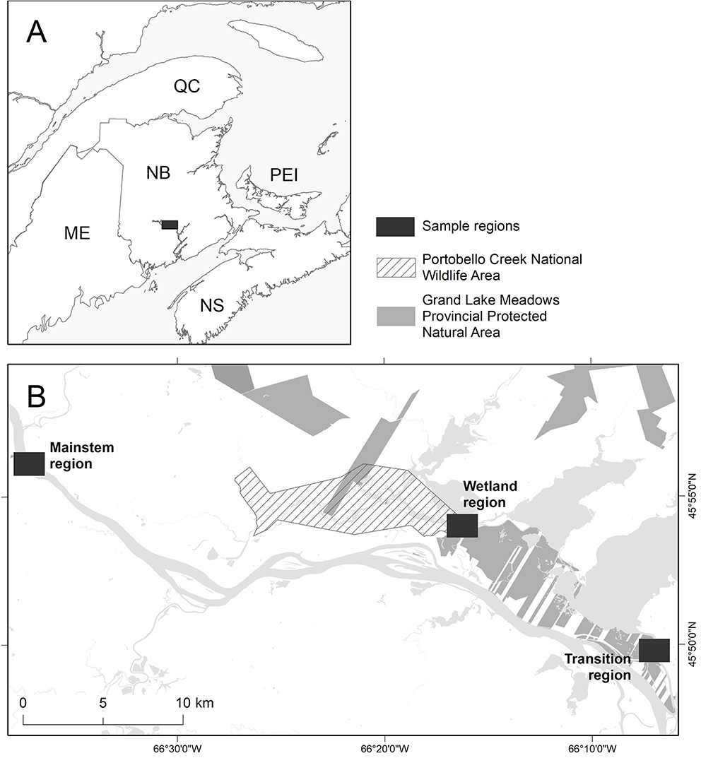
Figure 1. Map of the study area. (A) The Grand Lake Meadows complex, located in southern New Brunswick, is Atlantic Canada's largest freshwater wetland. (B) This complex is protected both nationally (diagonal lines) and provincially (light gray). Our study area consisted of three distinct regions (dark gray): the wetland (Wetland), the mainstem Saint John/Wolastoq River (Mainstem), and the Jemseg River (Transition), which connects the wetland to the mainstem region. Within each region, six sites were sampled three times (early June, early September, and mid-December).

Sites were sampled in early June, early September, and mid-December, 2016. We chose these time points because they represented the beginning, middle, and end of the active, ice-free season in our system. In the spring, ice break up occurs, creating large ice jams and massive spring flooding in the SJRW and GLM systems; consequently, June was the earliest point that we could sample with conditions returning to base flow. Peak productivity occurred in late-August into early September, and the active, ice-free season ended in mid-December during our final sampling event. Because major ice-flows scoured our system in spring of 2016, very little aquatic insect biomass was observed post-flood in June. Because of this, stable isotope samples were only collected in September and December, when there was enough biomass for sampling. Because early September (the peak of biological activity) and mid-December (when ice began reforming in our system) represented extremes in the biological activity in our system, the time points we selected for stable isotope sampling were expected to represent extremes in associated food webs and trophic dynamics.

At each site (n = 18, each sampled at three time points), paired benthic kick-net samples were collected using the standard protocol from the Canadian Aquatic Biomonitoring Network (CABIN; https://www.canada.ca/en/environment-climate-change/services/canadian-aquatic-biomonitoring-network.html): one sample for bulk sequencing and DNA metabarcoding of invertebrates, and a second sample for assessment of morphological identification of these taxa, organism body size, abundance, and analysis of stable isotopes (δ¹³C and δ¹⁵N). For bulk DNA samples, sterile technique was used and nets were sterilized between samples in a 1% bleach solution. DNA benthic samples (“DNA”) were preserved in 95% ethanol and stored at −80°C, but samples for microscopy and stable isotope analysis (“morphological”) were directly frozen (−20°C) on return to the lab, to avoid altering their isotopic composition (Arrington and Winemiller, 2002; Barrow et al., 2008). Additionally, samples for producer baselines were taken at each site, including detritus, biofilm, and dominant macrophytes; these samples were placed in paper bags and dried at 60°C in the lab for at least 72 h.

Laboratory Processing

Morphological samples were thawed and sorted, with invertebrates identified to the lowest taxonomic level (usually genus) using standard morphological keys (e.g., Merritt et al., 2008). Voucher samples and high-resolution digital images of key taxa are stored at the Environment and Climate Change Canada lab at the University of New Brunswick, Fredericton. Additionally, individuals were measured (total length, mm), and dried at 60°C. For stable isotope samples, all dominant taxa (based on biomass) were selected from samples covering all major functional feeding groups. Because of the mass requirements for stable isotope samples, we only included samples for taxonomic groups that had a dry biomass of ≥0.6 mg. This usually translated to each stable isotope sample including many individuals (>20); however, many predator groups were assessed from fewer individuals (often <3) because of the rarity of these taxa. Dried macroinvertebrate and food web base (i.e., biofilm, macrophytes, and leaf litter) samples were homogenized, weighed on a Sartorius MC21S microbalance (3.0 ± 0.1 mg for biofilm and plant tissue and 1.0 ± 0.1 mg for macroinvertebrate tissue), enclosed in 4 × 6 mm tin cups (Costech Analytical Technologies Inc., Valencia, California, USA), and delivered to the Stable Isotopes in Nature Laboratory (SINLAB) at the University of New Brunswick (http://www.unb.ca/research/institutes/cri/sinlab/) for stable isotope analysis.

Stable Isotope Analysis

Natural abundance stable isotopes of C and N were assessed for aquatic invertebrates and the food web base. Invertebrate and food web base ¹³C, ¹⁵N, C, and N content were measured using a Carlo Erba NC 2500 Elemental Analyzer (CE Instruments, Milan, Italy) with a Thermo-Finnigan Delta Plus XP (Thermo-Electron Corp., Bremen, Germany) isotope ratio mass spectrometer at SINLAB. Macroinvertebrate and food web base δ¹³C and δ¹⁵N isotope compositions were expressed in parts per thousand (‰) relative to Vienna PeeDee Belemnite for C and air for N, as follows:

$\begin{array}{ll}\delta =([{\text{R}}_{\text{sample}}/{\text{R}}_{\text{standard}}]-1)\times 1,000& (1)\end{array}$

where R is the ratio ¹³C/¹²C or ¹⁵N/¹⁴N. Instrumental error—measured as the standard deviation of repeated measurements of working laboratory standards (i.e., caffeine (δ¹³C = −35.05‰, δ¹⁵N = −2.87‰), bovine liver (δ¹³C = −18.8‰, δ¹⁵N = 7.2‰) and muskellunge liver (δ¹³C = −22.3‰, δ¹⁵N = 14‰))—was <0.1 ‰ for both δ¹³C and δ¹⁵N.

DNA Extraction and Sequencing

Benthic samples for DNA metabarcoding were packed on ice and shipped to the Biodiversity Institute of Ontario at the University of Guelph for DNA extraction, PCR amplification, and high throughput sequencing (HTS). Briefly, samples were homogenized in sterile blenders and the slurry was subsampled into 50 mL conical tubes. Samples were centrifuged, excess preservative ethanol was removed, and residual ethanol was evaporated at 65°C. Once dry, the homogenate was subsampled into 2 mL lysing matrix tubes (MP Biomedicals, Solon, Ohio) and further homogenized using a MP FastPrep-24 Classic tissue homogenizer (MP Biomedicals). Samples were then extracted using a NucleoSpin Tissue Kit (Machery-Nagel, Düren, German) according to the manufacturer's protocol, eluting with 30 uL molecular grade water. Samples were extracted in batches of 12–18 with a negative control (no sample added) for each batch.

Two COI fragments were amplified using the primer sets BR5 (B_F 5′ CCIGAYATRGCITTYCCICG, R5_R 5′ GTRATIGCICCIGCIARIACIGG−314 bp) and F230R (Folmer_F 5′ GGTCAACAAATCATAAAGATATTGG 230R_R 5′ CTTATRTTRTTTATICGIGGRAAIGC−230 bp) in a two-step PCR following the protocol outlined in Gibson et al. (2015), with the exception of having a 35 cycle regime in the first PCR. For both primer sets, the annealing temperature (Ta) was 46°C for 1 min. The melting temperatures (Tm) for these primers are as follows: BR5 (forward = 61.4°C, reverse = 56.4°C) and F230 (forward = 50.5°C, reverse = 56.7°C). For further information about these primers, which were designed to target a wide range of arthropod orders, see Gibson et al. (2015). A negative control was included for each batch of PCR, which was carried through each of the two PCR steps. Amplification success was confirmed visually using a 1.5% agarose gel. Amplicons were purified using a MinElute DNA purification system (Qiagen) and quantified using a Quant-iT (Invitrogen, Waltham Massachusetts, United States) PicoGreen dsDNA assay on a TBS-380 Mini-Fluorometer (Turner Biosystems Sunnyvale California, United States). All samples were normalized to the same concentration, and the two amplified fragments were pooled for each sample prior to dual-indexing using the Nextera XT Index Kit (Illumina, San Diego, California) (FC-131-1002). Indexed samples were pooled into one tube, purified through magnetic bead purification, and quantified using the PicoGreen dsDNA assay. Average fragment length was determined on an Agilent Bioanalyzer 2100 (Santa Clara, California, United States) before sequencing the library on an Illumina MiSeq using the V3 sequencing chemistry kit (2 × 300) (MS-102-3003). A 10% spike-in of PhiX was used as a control.

Bioinformatic Methods

Raw Illumina MiSeq paired-end reads were processed using the SCVUC v2.1 COI metabarcode pipeline, available on GitHub at https://github.com/Hajibabaei-Lab/SCVUC_COI_metabarcode_pipeline. At each step, read and ESV statistics were calculated (Supplementary Table S1) using custom scripts (available at the above link). Briefly, forward and reverse raw reads were paired using SEQPREP (available from https://github.com/jstjohn/SeqPrep) with a Phred quality score cutoff of 20 and an overlap of at least 25 bp (St. John, 2016). For each marker, forward and reverse primers were trimmed using CUTADAPT v1.14, ensuring trimmed reads were at least 150 bp long, allowing no more than 3 N's, and ensuring a minimum Phred quality score of 20 at the ends (Martin, 2011). A global ESV analysis was conducted by pooling all the data together, dereplicating the reads using VSEARCH v2.4.2 with the “derep_fulllength” command, and denoising with USEARCH v10.0.240 using the unoise3 algorithm (Edgar, 2016; Rognes et al., 2016). The denoising step removes sequences with predicted sequence errors, any PhiX carryover from MiSeq sequencing, putative chimeric sequences, and rare clusters. We defined rare clusters as exact sequence variant (ESV) clusters including only one or two reads (singletons and doubletons) (Callahan et al., 2017). A sample ESV matrix was generated using VSEARCH with the “usearch_global” command with an identity of 1.0 (100% exact sequence mapping, including matching of exact substrings). The denoised ESVs were taxonomically assigned using the COI classifier v3.2 (Porter and Hajibabaei, 2018; https://github.com/terrimporter/CO1Classifier).

Heuristic Food Web Construction

Heuristic food webs were constructed using a previously published pipeline (Compson et al., 2018). Briefly, this pipeline takes presence-absence taxonomic lists generated by DNA metabarcoding and pairs it with a customized interaction database covering the taxa found in our system. Our database of pairwise trophic interactions was created using a) information gathered from existing trophic databases (e.g., Database of Trophic Interactions; Brose et al., 2005), b) information from a secondary text-mining pipeline, and c) information manually gathered from systematic literature searches. Specifically, we used an updated trophic linkage database from Compson et al. (2018), which we updated to include novel taxa found in the GLM complex. Information gaps on species linkages, caused by missing species in our trophic interaction database, were inferred using a series of trait filters based on other information, including functional feeding group, body size, and phylogenetic relatedness. From the complete set of possible pairwise interactions, linkages were first reduced based on the known functional feeding group of each taxa, and then further reduced based on the average body size of each taxa. When functional feeding group or body size traits were not available, we obtained these traits from the next closest related species. The updated trophic linkage database includes 50,975 pairwise interactions and covers 965 invertebrate genera. Using this updated database, we created adjacency matrices by constraining interactions to only taxa present in a sample (for individual food webs) or region (for metawebs). We then used the cheddar R package (version 0.1-633; Hudson et al., 2013) to create food webs for each replicate sample and extract relevant food web metrics used for subsequent analyses.

Mixing Models for Trophic Position

Analysis of trophic position was done in two ways. First, we created a two-source, two-isotope Bayesian mixing model using the tRophicPosition position package (version 0.7.7; Quezada-Romegialli et al., 2018) in R to summarize trophic position of consumers in each of the dominant functional feeding groups in our system (i.e., predators, collectors, grazers, omnivores, and shredders) (Model 1):

$\begin{array}{ll}{\delta }^{15}{N}_{\text{c}}=\Delta N(TP-\lambda )+\alpha ({\delta }^{15}{N}_{\text{b}1}+{\delta }^{15}{N}_{\text{b}2})-{\delta }^{15}{N}_{\text{b}2},& (2)\end{array}$

where δ¹⁵N_c is the nitrogen isotopic ratio of the consumer, δ¹⁵N_b1 is the nitrogen isotopic ratio of the first baseline (biofilm), δ¹⁵N_b2 is the nitrogen isotopic ratio of the second baseline (leaf litter), ΔN is the trophic enrichment factor (TEF) for nitrogen, TP is the trophic position of the target consumer, and λ is the trophic position of the baseline. Additionally, this model uses a secondary mixing model to calculate α, which accounts for fraction in δ¹³C and estimates the relative contribution of each source to the consumer's trophic position:

$\begin{array}{ll}\alpha =([{\delta }^{13}{C}_{\text{b}2}-({\delta }^{13}{C}_{\text{c}}+\Delta C)]/(TP-\lambda ))/({\delta }^{13}{C}_{\text{b}2}+{\delta }^{13}{C}_{\text{b}1}),& (3)\end{array}$

where δ¹³C_c is the carbon isotopic ratio of the consumer for which we want to estimate trophic position, δ¹³C_b1 is the carbon isotopic ratio of the first baseline (biofilm), δ¹³C_b2 is the carbon isotopic ratio of the second baseline (leaf litter), and ΔC is the TEF for carbon. The Bayesian approach allows Equations (2) and (3), which both include TP and α, to be solved iteratively, with δ¹³C and δ¹⁵N values and TEFs for both consumers and baselines modeled as random variables with vague prior normal distributions of their means [dnorm(0,τ), τ = 1/SD²] and vague prior uniform distributions of their standard deviations [dunif (1,100)]; TP and α are treated as random parameters with uniform and Beta prior distributions, respectively (Quezada-Romegialli et al., 2018). We used the function “multiSpeciesTP” to define and initialize the Bayesian model, and to sample the posterior distribution of trophic position. The Bayesian model ran 10,000 iterations used for the parameters “n.adapt,” “n.iter,” and “burnin” and used five parallel Markov Chain Monte Carlo (MCMC) simulations using the JAGS (version 4.3.0) Gibbs sampler (Plummer, 2003).

The second approach we employed for calculating trophic position (TP) was a more conventional model (Model 2; Post, 2002):

$\begin{array}{ll}TP=\lambda +({\delta }^{15}{N}_{\text{c}}-[{\delta }^{15}{N}_{\text{b}1}\times \alpha +{\delta }^{15}{N}_{\text{b}2}\times (1-\alpha )])/\Delta N.& (4)\end{array}$

Here, α is defined as,

$\begin{array}{ll}\alpha =({\delta }^{13}{C}_{\text{c}}-{\delta }^{13}{C}_{\text{b}2})/({\delta }^{13}{C}_{\text{b}1}-{\delta }^{13}{C}_{\text{b}2}).& (5)\end{array}$

This model allowed us to calculate individual trophic position values for all consumers in our system, including those taxa represented by few individuals; Bayesian models, which require replicate observations for each consumer estimated, could only provide group-level estimates and confidence intervals for well-represented individuals and functional feeding groups across food webs. Consequently, trophic position values obtained from Model 2 were used for all linear regression analyses. For both Model 1 and Model 2, TEFs were based on values for whole organisms reported in McCutchan et al. (2003). Additionally, for predators, we explored models using consumers as the baseline, which involved changing the baseline trophic position from λ = 1 (for biofilm and detritus) to λ = 2 for consumers feeding primarily on biofilm (i.e., grazers) and terrestrial leaf litter (i.e., shredders). Finally, from trophic position (TP) estimated from Model 2, we also calculated adjusted trophic position (ATP), which used known information about the habits of each organism or functional feeding group to constrain trophic position to not go below these trophic levels (i.e., λ = 2 for consumers and λ = 3 for predators).

Bayesian Estimates of Isotopic Food Web Size

To compare how community-wide trophic niche breadth varied spatially and temporally, we used the SIBER R package (version 2.1.4; Jackson et al., 2011). Specifically, we examined the Bayesian posterior estimate of the convex hull area of each community, which encompasses all species in δ¹³C-δ¹⁵N bi-plot space and is a measure of the total amount of niche space occupied by the community (Layman et al., 2007). The Bayesian model utilized a JAGS Gibbs sampler with five MCMC chains. This model fit initial multivariate normal distributions to each group in the dataset with rjags (version 4-8), using the recommended default SIBER parameters and priors (Jackson et al., 2011). The default priors included an inverse Wishart prior for fitting ellipses and a vague normal prior for the means; vague normal priors are recommended for fitting the means because SIBER internally z-score standardizes the data before model fitting, aiding in the JAGS fitting process (Jackson et al., 2011). Because of spatial and temporal variation in our producer baselines (Supplementary Figure S1, Supplementary Table S2), prior to running Bayesian models we converted our δ¹³C data to autochthonous reliance values (0–1) and our δ¹⁵N data to trophic position values (based on Model 2).

Statistical Analyses

All statistical analyses were conducted in R (version 3.6.0; R Core Team, 2013). To assess the spatial and temporal variability in heuristic food web metrics, including estimates of trophic position, we created a linear mixed effects model using the lme4 package (version 1.1-21; Bates et al., 2019), where Season and Region were fixed effects, and Site was a random effect nested in Region. Contrasts were set up a priori to maximize comparisons across the different levels of the individual terms and interactions. Model terms and interactions were assessed using both t values and calculated statistical significance using Satterthwaite's method for approximating the degrees of freedom using the lmerTest package (version 3.1-0, Kuznetsova et al., 2017).

Linear regression analyses were used to assess how well-trophic position measured from heuristic food webs predicted trophic position measured from stable isotope values. First, we extracted trophic position values from all food webs, including metawebs, using the TrophicLevels function in the cheddar package (version 0.1-633; Hudson et al., 2013). This function provides multiple estimates of trophic position for each node in the food web, including prey averaged trophic position (PATP) and chain-averaged trophic position (CATP) (Levine, 1980; Cohen et al., 2003; Williams and Martinez, 2004; Jonsson et al., 2005). We then paired these values with trophic position estimates from stable isotope values (Model 2, Equations 4 and 5) according to taxa (at the genus level) and conducted separate analyses with different predictor (i.e., PATP and CATP) and response (i.e., TP and ATP) variables. Model significance was assessed using p-values (α = 0.05), and models were compared qualitatively using R² statistics.

Results

Heuristic Food Webs

Heuristic food webs constructed from DNA and paired trait information elucidated both spatial and temporal patterns in the GLM complex. Metawebs (i.e., food webs aggregated across samples) from the wetland region of the complex were relatively larger (i.e., more nodes), denser (i.e., higher connectance), and had a higher maximum trophic position (due in part because of more predators) than metawebs from the transition and mainstem regions of the complex; metawebs from the transition region were generally the smallest and sparsest, with lower numbers of nodes, links, and maximum trophic positions compared to metawebs of the other regions (Figure 2). Metawebs generally constricted through time, such that they got smaller moving from early June, to early September, to mid-December; however, metawebs from the transition region of the GLM complex were the smallest, least complex food webs overall, and varied little over the study period (Figure 2).

FIGURE 2

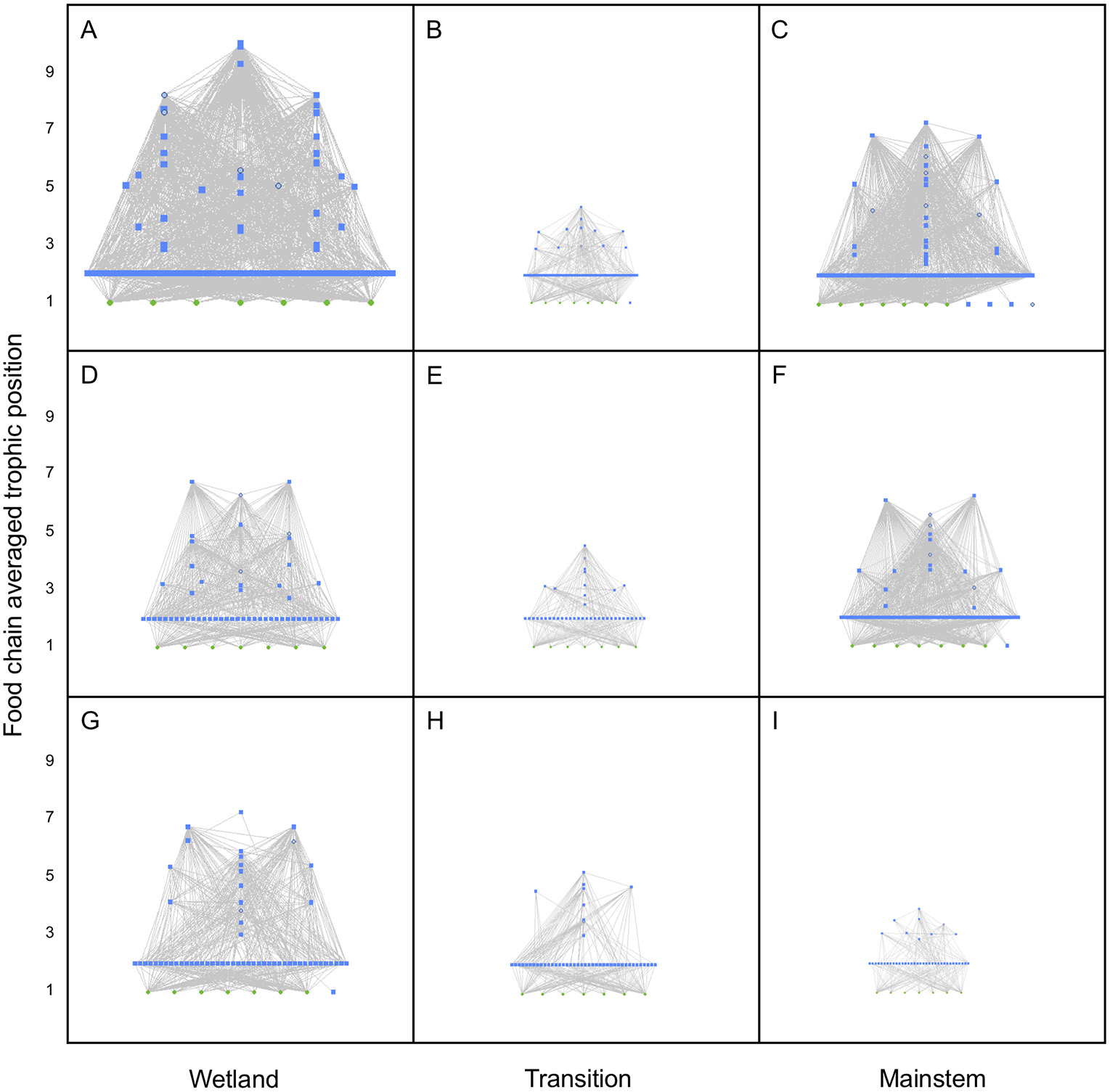
Figure 2. Metawebs for the Portobello Creek wetland complex (Wetland), the Jemseg River connecting the wetland to the mainstem (Transition) and the Saint John/Wolastoq River (Mainstem) in (A–C) June, (D–F) September, and (G–I) December of 2016. Trophic position for each node was calculated as the food chain-averaged value for that consumer or resource. For nodes, green squares depict producers, blue squares depict consumers, and open blue circles depict cannibalistic consumers. The size of nodes and thickness of links are scaled to the maximum trophic position for each food web.

Assessment of food web properties across individual heuristic food webs revealed seasonal but little spatial variation. The strongest patterns appeared to occur between June and December, but differences between other months were also apparent (Supplementary Table S3, Figure 3), with September exhibiting the most variation in food web metrics compared to the other months (Figure 3). Spatial patterns were weaker, with no significant Region terms for any of the metrics and Site variation explaining only a small amount of the residual variation via the random effects, but there were Season^*Region interactions for the number of trophic links and chain-averaged trophic level (Supplementary Table S3).

FIGURE 3

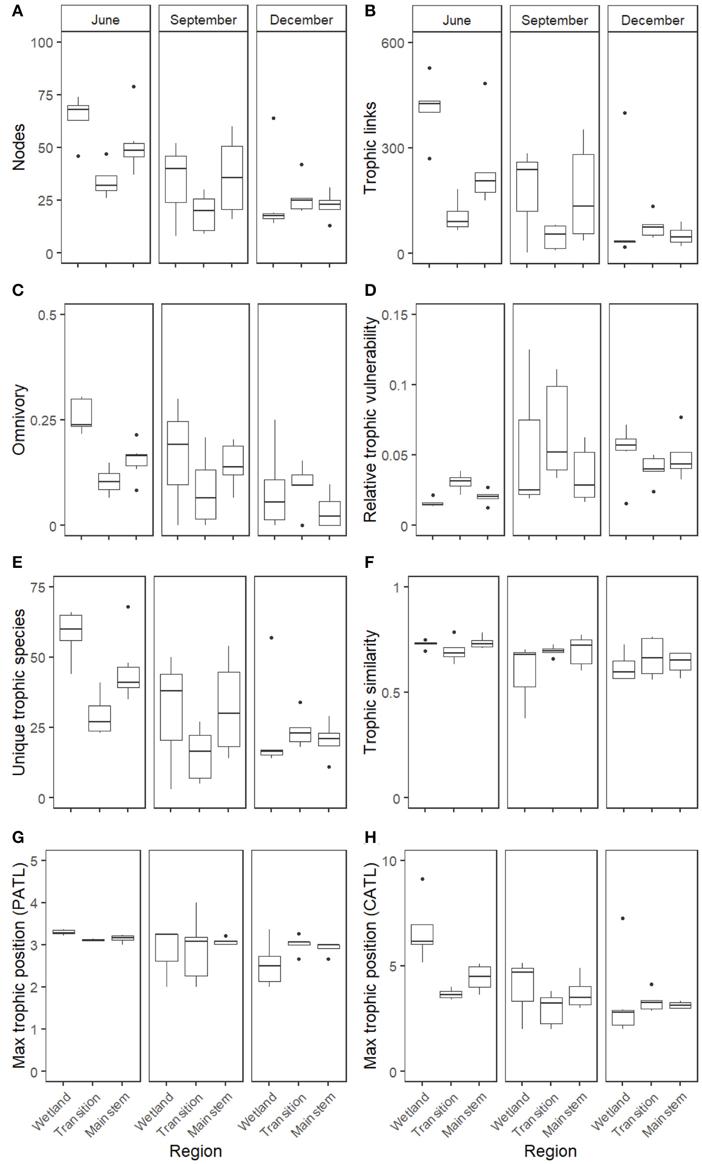
Figure 3. Boxplots of the eight measured heuristic food web properties, expressed across the three regions of the GLM complex (Wetland, Transition, and Mainstem) and across the three seasons of the study (June, September, and December). Food web metrics included the following whole-network properties: (A) the number of nodes, (B) the number of trophic linkages among nodes, (C) the proportion of omnivory, (D) relative trophic vulnerability, or the average vulnerability across all nodes, standardized by the number of trophic linkages, (E) the number of unique trophic species, (F) the trophic similarity measured across all nodes, (G) the maximum prey-averaged trophic position, and (H) the maximum chain-averaged trophic position.

Stable Isotope Analysis of Trophic Position and Community Niche Width

Bayesian estimation of trophic position using stable isotopes (Model 1, Equations 2 and 3) revealed no significant seasonal differences in maximum trophic position (i.e., the trophic position of predators) between September and December (Supplementary Table S4). However, when the model was run with primary consumers as the baseline instead of the food web base (i.e., leaf litter and biofilm), trophic position of predators was significantly lower in the wetland region in December compared to September (Supplementary Table S4). This, however, was the only significant pattern revealed by Bayesian analysis of trophic position (Supplementary Table S4). Because Bayesian mixing models are very different from linear mixed effects models and stable isotope data were only collected in September and December, we also qualitatively assessed maximum trophic position assessed from stable isotopes (Model 2, Equations 4 and 5) with maximum trophic position assessed from heuristic food webs using a series of reduced linear mixed effects models (Supplementary Table S5). These results indicated that the stable isotope approach showed differences in maximum trophic position in September compared to December, while heuristic food webs did not (Supplementary Table S5). Similar to Bayesian and full linear mixed effects models, these reduced models failed to show any significant effects among regions (Supplementary Table S5).

Invertebrate community trophic niche widths varied little spatially and temporally (Figure 4). In general, trophic niche widths were slightly larger for all regions in December—when trophic positions were also higher for all regions (Figure 4A)—compared to September, but these differences were not strong as the 95% confidence intervals for all regions and seasons overlapped (Figure 4B). While the trophic niche widths did not change spatially or temporally, energy pathways did change among regions through time (Figure 4A). Communities in the wetland and transition regions, for example, both increased in their autochthonous reliance moving from September to December; communities in the mainstem region, however, decreased in their autochthonous reliance moving from September to December (Figure 4A). In general, communities in the mainstem region were fueled by autochthonous resources in September, but shifted toward a mixture of autochthonous and allochthonous resources in December, while communities in the wetland and transition regions relied on both autochthonous and allochthonous resources in September and increased in their reliance on autochthonous resources in December (Figure 4A).

FIGURE 4

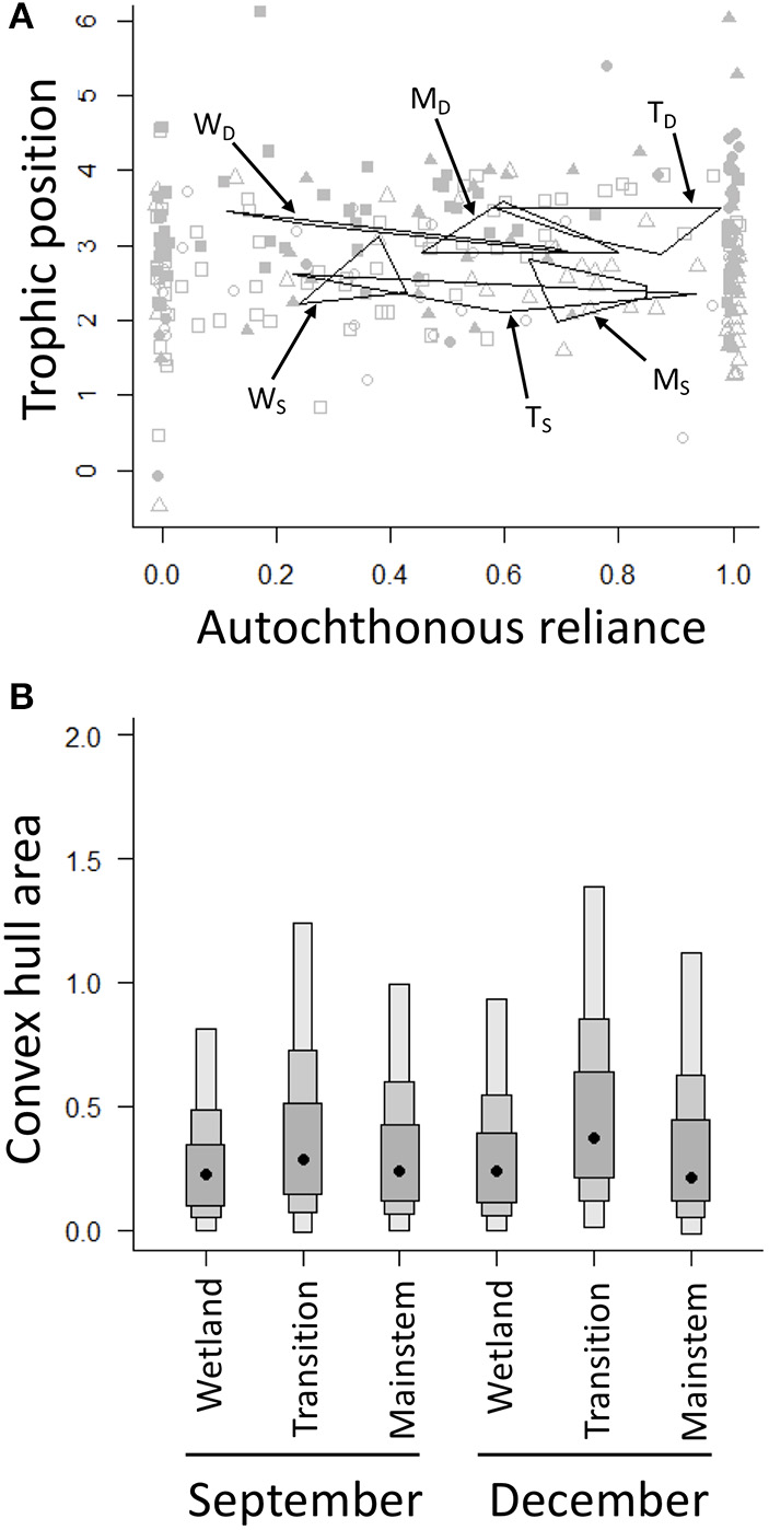
Figure 4. (A) Convex hulls for the three regions of the GLM complex in September [open squares = wetland (W_S), open circles = transition (T_S), open triangles = mainstem (M_S)] and December [filled squares = wetland (W_D), filled circles = transition (T_D), filled triangles = mainstem (M_D)]. Convex hulls are based on the centers of each of the functional feeding groups that make up each community. (B) Density plots of the convex hull area are based on posterior estimates from Bayesian mixing models analyzed using the R package SIBER. Black dots depict group modes, and the shaded boxes represent the 50% (dark gray), 75% (gray), and 95% (light gray) confidence intervals.

The Relationship Between Estimated and Measured Trophic Position

Trophic position estimated from heuristic food webs was generally a strong predictor of trophic position estimated from stable isotope values (Supplementary Table S6). Prey-averaged trophic position (PATP) was consistently the strongest predictor of trophic position estimated from stable isotope values, exhibiting the highest R² values across models (seasonal models, R² range: 0.51–0.78; global models, R² range: 0.48–0.60). The strength of the relationships generally increased for predictions of adjusted trophic position (ATP) (Supplementary Table S6), as this variable constrained trophic position estimates based on knowledge of the minimum possible trophic position of a consumer. The global model predicting ATP (including all paired samples across all regions and seasons) was significant for both maximum PATP (R² = 0.60, p < 1.00 e-15; Figure 5A) and maximum chain-averaged trophic position (CATP; R² = 0.38, p < 1.00 e-15; Figure 5C), and these relationships were generally stronger for specific regions at specific time periods (PATP R² range: 0.58–0.78; CATP R² range: 0.34–0.62). For these models, the deviation in predicted and measured trophic position varied based on functional feeding group. For example, the best predictor (i.e., PATP) tended to underestimate the trophic position inferred from stable isotopes for filter-feeders, but predictions closely matched for collector-gatherers, shredders, and predators, the latter which exhibited the lowest amount of variation in trophic deviation (Figure 5B). Trophic deviation patterns changed when CATP was used as the predictor, which tended to better predict the trophic position of functional feeding groups closer to the base of the food web and over predict the trophic position of functional feeding groups at higher trophic levels (Figure 5D). Finally, across all individual food webs, models that only included the maximum trophic position of each food web revealed that heuristic food web estimates significantly predicted the maximum trophic position estimated by stable isotope analysis (Supplementary Table S6, producer baseline models; all p < 0.05), but that these patterns were relatively weak (R² range: 0.13–0.17); these patterns, however, did not hold when consumer baselines were used in trophic position models instead of producer baselines (Supplementary Table S6, consumer baseline models; all p > 0.05).

FIGURE 5

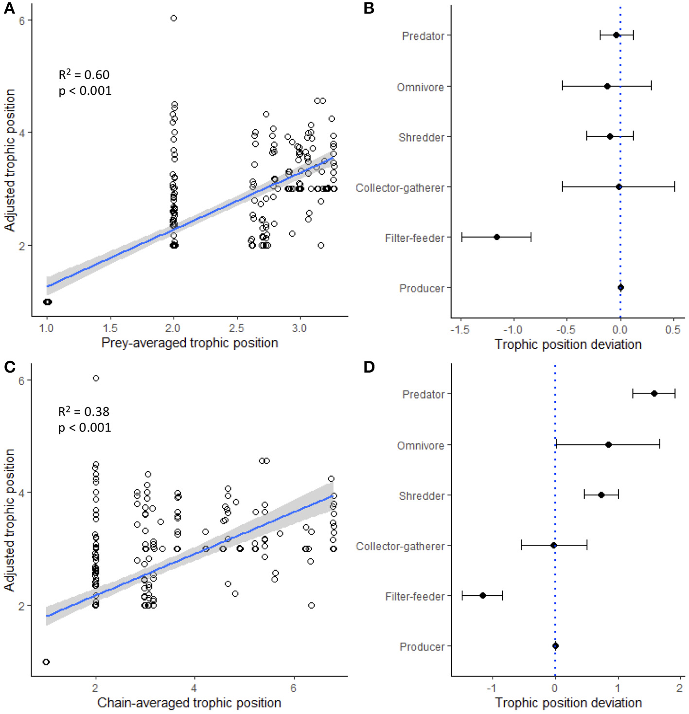
Figure 5. Global linear regression models illustrating how well two heuristic food web estimates of trophic position [(A) prey-averaged trophic position and (C) chain-averaged trophic position] predicted trophic position inferred from stable isotope analysis. Points have been jittered for visualization purposes. (B,D) Deviation of different functional feeding groups are indicated by black dots with 95% confidence intervals; negative values indicate when heuristic food web analysis underestimated stable isotope trophic position, and positive values indicate when heuristic food web analysis overestimated stable isotope trophic position.

Discussion

The Predictive and Discriminatory Power of Heuristic Food Webs

We have demonstrated that heuristic food webs can provide a reliable and powerful tool for the characterization of invertebrate community structure and assessment of spatial and temporal differences among the wetland, transitional, and mainstem regions of the GLM complex. Metawebs of the three regions indicated that all food webs became less connected moving from June to September to December, and that the largest spatial differences across regions were in June and December, where the wetland trophic network was clearly larger and denser than transition and mainstem networks. Analysis of individual food webs indicated that temporal patterns were more pronounced than spatial patterns. All the food web properties we examined showed significant variation seasonally, whereas none showed significant spatial variation, though there were significant Region^*Season terms for both trophic links and chain-averaged trophic position (Supplementary Table S3). These results support those found in another study examining DNA-based heuristic food webs in a different wetland complex, the Peace-Athabasca Delta, in northern Alberta (Compson et al., 2018). Given that extensive flooding in both the Peace-Athabasca Delta and GLM complex are regular events, connecting the wetlands to the main river channels, perhaps it is not surprising that these aquatic habitats can appear structurally homogeneous (Thomaz et al., 2007). However, the apparent contradiction between our metawebs, which showed clear structural differences among regions, and analysis of individual food webs suggests that it is more likely that spatial variability among sites within these regions was high, and this was certainly the case at all sites in September (Figure 3). This highlights one of the key advantages of metawebs as a visualization tool for biodiversity and community structure: while they do not convey the site-level variation within a region, because they are an aggregator of all detected biodiversity in a system, they give an overview of how these taxa are structured and interact trophically, providing scientists with a tool for making predictions about how a system might respond to perturbations (e.g., species extirpations or invasions, changes in resource availability, anthropogenic impacts) and how ecosystems function (reviewed in Thompson et al., 2012).

Stable isotope analysis generally confirmed the spatial and temporal patterns revealed by our heuristic food web analysis. For example, our Bayesian mixing models (Model 1, Equations 2 and 3) demonstrated that predators had a significantly higher trophic position in September compared to December at sites in the wetland region, but that there were no spatial differences in the trophic position of predators or any other consumers. Given that we only collected stable isotope samples in September and December, a more direct comparison of how well-heuristic food webs and stable isotopes resolved spatial and temporal patterns is a qualitative assessment of the reduced linear mixed effects models (Supplementary Table S5). Again, analysis of trophic position calculated from stable isotope values (Model 2, Equation 4 and 5) indicated that maximum trophic position only varied seasonally, and that there were no spatial differences. Interestingly, the two food web metrics we examined (i.e., prey-averaged trophic position and chain-averaged trophic position) differed neither spatially nor temporally using the reduced linear mixed effects models (i.e., using only September and December data) (Supplementary Table S5). Here, the discrepancy of the two approaches could have arisen because the maximum trophic position measured using stable isotopes is based on the single, highest value of all taxa examined in the community, whereas both heuristic food web metrics for maximum trophic position are integrated estimates of all the possible links to the top predator, meaning that the heuristic approach is a more integrated estimate across the entire food web. Additionally, these differences could have arisen because of our sampling design, since we targeted functional feeding groups with sufficient biomass to support stable isotope analysis. While we assessed all predators in our samples in order to get the best estimate of maximum trophic position, this approach means that in September, when we found many more predators than in December, we increased our chances of finding a single predator with a high trophic position value, potentially exacerbating differences between September and December. This illustrates why Bayesian mixing models, which integrate variation in trophic position across all predators (or other functional feeding groups), are a more robust approach for measuring trophic position compared to point estimates from simpler mixing models. Similarly, heuristic food webs, which are created from DNA-metabarcoding data of the entire community in the sample, are likely to be a more robust estimate of maximum trophic position, as these estimates integrate all members of the community and are less biased to subsampling of larger individuals.

One of the most promising results emerging from this study was the finding that trophic position measured from heuristic food webs predicted trophic position inferred from stable isotope analysis. Significant variation was explained when measured across all paired samples (i.e., global models, R² range: 0.31–0.60; all models p < 0.05), which improved further (R² range: 0.34–0.78, all models p < 0.05) when the analysis was constrained within the metaweb of a specific region and season (Supplementary Table S6, Figure 5). One caveat of these models is that the cluster of points at the baselines has a strong leveraging effect on the linear patterns; when we examined the models with the baselines removed, patterns were generally weaker (data not shown). Further, when we explored models for individual functional feeding groups or maximum trophic position, patterns were much weaker and often not significant (Supplementary Table S6). Consequently, it is likely that heuristic food webs will do a better job at predicting the trophic structure of an entire community and not necessarily the specific trophic position of individual consumers or functional feeding groups. However, it is important to emphasize that deviation from these linear patterns was predictable, especially for some functional feeding groups. For example, models using prey-averaged trophic position consistently underestimated the trophic position of filter-feeders, while other groups were much more consistently predicted (Figure 5B). These findings suggest the possibility of calibrating heuristic food webs using stable isotope data. While it is impractical—if not impossible—to collect stable isotope data for all members of a community, our findings suggest that collecting samples from a few key functional feeding groups could allow the trophic position of some groups to be better predicted by heuristic food web analysis. Importantly, despite some groups (e.g., collector-gatherers, omnivores) exhibiting a wide range of variation in their deviation from these linear predictions, estimates of trophic position for invertebrate predators exhibited the least deviation, perhaps because they obtain biomass from many different chains in a food web.

Given that our heuristic food web and stable isotope analyses did not assess fish and other vertebrate predators feeding higher in the food web, these taxa represent important groups for future case studies linking ecological network and stable isotope approaches. Based on our findings, which indicate that heuristic food webs best predict the trophic position of invertebrate predators in models covering a wide range of functional feeding groups, we hypothesize that including vertebrate predators in these food webs will (a) improve whole-food web regression models of trophic position, and (b) lead to more accurate estimates of trophic position of these vertebrate top predators, with less trophic deviation, compared to invertebrate predators and consumers. These hypotheses are contingent upon the scale of the study, the hydrological connectivity of the system, seasonal flow dynamics, and the disbursal and trophic specialization of the taxa studied. For example, in hydrologically distinct systems where vertebrate predators are disbursal limited or have narrow trophic niches, trophic position estimates of these predators will likely be the most accurate, while they should be relatively weaker in hydrologically interconnected systems with mobile, generalist predators. A larger-scale study—covering a wider range of spatially and hydrologically distinct systems—would likely be needed to assess patterns of mobile predators like fish. However, given the hydrological interconnection of the GLM complex and the extreme seasonal dynamics of this system, the strong trophic position patterns we demonstrate for invertebrate predators shows the promise of the heuristic food web approach, even when ideal conditions are not met. If the trophic deviation patterns we demonstrate hold in different systems, heuristic food webs might live up to the promise of being a rapid indicator of both trophic structure and trophic dynamics, which would be especially useful in biodiverse systems that are difficult to study.

Merging DNA Metabarcoding and Ecological Network Analysis

Measuring food webs poses a great challenge. Constructing a food web requires the ability to sample and identify every species in a system and then to determine, or at least infer, all the trophic interactions among these species, which requires further information about species traits (reviewed in Thompson et al., 2012). These challenges illustrate why so few quality food webs have been described in the literature (Dunne et al., 2002a). Here, we have demonstrated the utility of employing a food-web generating pipeline based on DNA-derived biodiversity knowledge (Compson et al., 2018). Food webs can be generated in this manner in a fraction of the time that would otherwise be needed to quantify a trophic network, especially those as complex as wetland food webs (Halls, 1997; Millennium Ecosystem Assessment, 2005); yet, the quality and coverage of trait information available for the breadth of biodiversity in trait databases remains heterogeneous and incomplete (reviewed in Schneider et al., 2019). Our pipeline was therefore based on many assumptions about species interactions (detailed in Compson et al., 2018). Nonetheless, the generated heuristic food webs performed well as predictors of trophic position derived from stable isotope analysis, and exhibited similar spatial and temporal patterns in trophic position compared to those revealed by stable isotope analysis.

Exploring the composition of biological communities based on their DNA signature permits rapid acquisition of sequence-based occurrence data and thus orders of magnitude more taxonomic information when compared with traditional microscope-based taxonomy (Gibson et al., 2015). When this high-resolution biodiversity information is organized into ecological networks, it yields even more information on connections among organisms and how this structures the food web; understanding the variation in this connectivity can reveal complex ecological relationships (Winemiller, 1989; Dunne et al., 2002b; Poisot and Gravel, 2014). Indeed, while ecological networks have long been proposed as inexpensive tools for assessment of biostructure (McCann, 2007), the added resolution DNA-based networks provide can improve their use as a tool, and even radically change the inferences we make (Wirta et al., 2014). What is more, using DNA metabarcoding to assess communities does not always require direct observation of interactions, as gut contents, blood meal, or feces, for example, can be sequenced and interactions inferred directly from DNA metabarcoding results, circumventing the need for laborious field observations, rearing experiments, or gut content analysis (Clare et al., 2019). For this reason, genomics approaches are particularly useful for resolving difficult trophic situations, such as those involving hard to identify taxa, relationships involving cryptic species, or interactions with fluid feeders. These potential advantages of DNA-based ecological networks are opening a new frontier in ecosystem monitoring, permitting exploration of how networks change through space and time in other ecosystems and, importantly, across stronger gradients of environmental change. Our study demonstrated that strong seasonal gradients dominate in the GLM complex, but this system is relatively unimpaired and is hydrologically connected, so it is not surprising that stronger spatial patterns were not observed among regions. Further, while our study explored one important food web metric—trophic position—it is unclear how this and other food web metrics will relate to ecosystem function. Certainly, network metrics provide a promising opportunity to develop novel indicators (sensu Kissling et al., 2018) of ecosystem change¹.

Stable Isotope Analysis and DNA-Based Ecological Network Analysis: Complimentary Approaches

One of the more interesting results that emerged from this study was how the unique information from heuristic food web analysis and stable isotope analysis provided surprising, yet complementary results, illuminating the complexity of the food webs in the GLM complex. While heuristic food web analysis provided both visual and quantitative data on the relative structure, size, and complexity of the food webs in the three regions of our study, stable isotope analysis illuminated the trophic niche widths and energy pathways of communities in these regions. For example, while trophic niche widths (based on stable isotope analysis) differed neither seasonally nor spatially in our system (Figure 4B), metawebs (based on heuristic food web analysis) were clearly larger in the wetland region, and across all regions, became generally smaller later in the year (Figure 2). One of the explanations for these findings is that heuristic food webs measure all of the organisms DNA can detect in a system, whereas stable isotope analysis in our study considered only dominant taxa (i.e., taxa with enough abundance or biomass to constitute a composite isotope sample), and this could mean that while a lot of the rare or non-dominant taxa were reduced (at least below the levels of DNA detectability) later in the season, the core food web backbone (sensu Serrano et al., 2009; Lu et al., 2016) was more resilient to seasonal change in our system, an idea that is beyond the scope of this study but that warrants more attention. Future studies might be able to use network principles (e.g., the friendship paradox; Pires et al., 2017) to identify highly connected species critical to food webs prior to sampling the entire network, which could aid in project development, enabling researchers to identify key community members of a food web to sample for stable isotope analysis.

Another example of the complementary information stable isotope and heuristic food web analyses provide is the finding that—despite the lack of differences in trophic niche widths across space and time—stable isotopes revealed a shift in autochthonous reliance from September to December: the wetland and transition regions generally increased in autochthonous reliance moving later into the year, while the mainstem region decreased in autochthonous reliance (Figure 4A). It is possible that these differing patterns in resource use could reflect the different flow and productivity dynamics in the three regions of the GLM complex. In the highly productive wetland and transition regions, where allochthonous litter subsidies are probably exhausted or buried in sediments later in the year, leaf litter is likely less important in the winter; however, in the mainstem region, where flows are much higher and ice cover takes longer to establish, tributaries of the SJWR likely deliver a relatively high allochthonous subsidy later in the year. Consequently, while food webs were getting relatively smaller across the regions of the GLM complex throughout the year, the dominant energy pathways of the food webs changed in different regions and in different ways, indicating that seasonality, and potentially other disturbances that reduce food web size (e.g., Lu et al., 2016), could impact the structure and function of these ecosystems differently. It should be noted that while our study used aggregate samples (i.e., many individuals of a particular taxon made up an isotope sample), one advantage of stable isotope analysis compared to heuristic food web analysis is that, when a single sample is taken for each individual, it is possible to measure the variation among individuals in a population, enabling the elucidation of intraspecific energy flow pathways, especially for larger bodied consumers, like fish; in studies where a more nuanced energy flow assessment is the aim, the stable isotope and heuristic food web approaches will provide even more complementary information, with heuristic food webs providing a broad picture of how all of the organisms in a food web are connected, and stable isotope analysis elucidating specific pathways of interest.

Collectively, the complementary information gleaned from stable isotope and heuristic food web analyses may indicate important ways communities in the GLM complex function and utilize resources. Intra- and interspecific competition, ecological opportunity, and predation all govern among-individual niche variation, which likely both affects and is affected by community dynamics (Araújo et al., 2011). Because these mechanisms can be affected by seasonality in wetlands, where the flood regime and seasonal drying can exert strong pressures on organisms and communities (Costa-Pereira et al., 2017), they also likely influence community niche width, which is linked to ecosystem function (Salles et al., 2009). In the GLM complex, which is subject to late-season drying and early winter ice formation, these seasonal processes can act to both decrease ecological opportunity by reducing habitat connectivity and increase competition by reducing resource availability, two processes that would have opposite effects on community niche width. This supposition is congruent with our findings that trophic niche width differed among regions in neither September (when habitat connectivity was reduced due to late season drying) nor December (when habitat connectivity was further reduced by ice formation), and likely the reduced habitat connectivity by these events limited any increase in trophic niche width that could have arisen from increased competition. Our findings differed from those of another study in the Pantanal wetland, where habitat constriction in the dry season led to reduced niche width in a tetra fish population despite increased competition (Costa-Pereira et al., 2017). The differing patterns found in our study could be attributed to the fact that habitat constriction likely impacts the niche width of fish, which are relatively mobile, more than invertebrates, especially at the scales examined in our study.

Our results illustrate the complementary nature of DNA-based network analysis and stable isotope analysis. Stable isotope analysis provides a longer-term picture of energy flow patterns of key or dominant taxa, while DNA-based heuristic food web analysis provides a high-resolution snapshot in time of the entire community of interest. These two approaches will likely be synergistic in cases where (1) multiple pressures drive biodiversity and trophic patterns differently, (2) direct observation of trophic interactions cannot be made, (3) a community has a lot of cryptic species that are in competition or could undergo niche differentiation, (4) general energy flow pathways can be established with stable isotope mixing models, but more resolution is required to elucidate the players responsible for these patterns (e.g., DNA metabarcoding the gut contents of fish or riparian predators to better resolve aquatic-terrestrial linkages), and (5) researchers exploring heuristic food web analysis require additional evidence about interaction strengths among linkages. Of these potential synergies, the latter is probably the most challenging, especially in complex food webs, because while heuristic food webs can accommodate an unlimited number of basal food web resources, even the most sophisticated isotopic mixing model is mathematically constrained by the number of isotopic tracers in the system, which must also exhibit isotopically distinct signatures (Fry, 2006). Even in cases where food webs are very complex, however, stable isotopes could elucidate the food web backbone (sensu Serrano et al., 2009), such that dominant energy pathways of a food web are quantified. Certainly, interaction strengths among nodes of heuristic food webs could be quantified in other ways, including through added abundance or biomass information (Thompson et al., 2012), mathematical occupancy modeling with replicate DNA metabarcoding samples (Doi et al., 2019), probabilistic models of interaction (Morales-Castilla et al., 2015), or even using relative read abundances (Deagle et al., 2019). How much this added information will improve heuristic food web predictions of ecosystem structure and function remains to be seen and will likely vary based on ecosystem type and spatial and temporal scales, but this question is at the forefront of the field of ecological network analysis.

Overcoming the Limitations of DNA-Based Heuristic Food Webs as a Rapid Bioassessment Tool

Ecological network analysis has long been argued to be a tool that could provide inexpensive analysis of biostructure (McCann, 2007), and with the advent of next-generation sequencing approaches, this tool has the potential to be part of an analytical pipeline for rapid bioassessment (Gray et al., 2014; Bohan et al., 2017). At the time of writing, we were unaware of any international jurisdiction which is actively employing DNA metabarcoding for biomonitoring purposes or ecological network analysis. Heuristic food webs—which take ecological co-occurrence networks and build upon them by integrating known or measured trait information, such as information about feeding habits, species interactions, or stable isotopes—present challenges for use as a rapid bioassessment tool, despite the clear advantages they provide over simple co-occurrence networks (e.g., calculation of food web metrics, such as trophic position or relative network vulnerability).

We have identified five key advances that will overcome many of the limitations preventing widespread adoption of DNA-based heuristic food web analysis as a tool for rapid bioassessment. (1) A more widespread adoption of genomics tools is needed, particularly among groups in charge of biomonitoring programs. As standardized field sampling methods are established for environmental genomics sampling (e.g., see CABIN and National Ecological Observatory Network protocols), DNA sequencing technologies are advanced (Singer et al., 2019), genomics laboratory procedures are refined, and primers are optimized (sensu Hajibabaei et al., 2019), the cost of implementing genomics approaches will come down and public adoption should increase, but technological advancements are not often readily adopted by resource managers and policy makers (Darling and Mahon, 2011). Consequently, more needs to be done to improve biomonitoring of aquatic ecosystems by bringing stakeholders together, such as GEO BON (www.geobon.org), GEOSS (www.earthobservations.org), COST action DNAqua-Net (www.dnaqua.net), and SYNAQUA (www.interreg-francesuisse.eu) (Hering et al., 2018; Leese et al., 2018; Lefrançois et al., 2018; Pawlowski et al., 2018). (2) Bioinformatics pipelines need to be developed, reviewed (sensu Mangul et al., 2019), and made publicly available via open-source archival services, like GitHub or SourceForge, and through package managers, like Bioconda (Grüning et al., 2018). (3) Open-source databases for both genomic (e.g., BOLD, GenBank) and trait data (e.g., GloBI, EPA's Freshwater Biological Traits Database) need to be improved. Currently, the coverage of these databases is lacking, especially for understudied systems (Compson et al., 2018; Curry et al., 2018), but efforts to develop and integrate databases for ecological network analysis are underway (e.g., Poisot et al., 2016; Vissault et al., 2019). (4) We require more case studies demonstrating the utility of DNA-based network and food web analyses and the meaning of their derived network metrics. Testing these tools will be important in novel ecosystems, across extreme environmental gradients, and across large spatial and temporal scales, especially in cases where we can pair these assessments with measured estimates of ecosystem function. (5) To facilitate these efforts and to house and curate the massive amount of data next-generation biomonitoring will generate (sensu Hey and Trefethen, 2003; Bell et al., 2009), an international biomonitoring consortium needs to emerge, with federated centers for data aggregation¹. Promisingly, advancements in any one of these areas will improve the utility and adoption of DNA-based network approaches, as progress in these areas will be linked but not necessarily limited by uneven advancement. Collective advancements made on these five fronts will enable heuristic food webs to steadily improve in their resolution, utility, and predictive power.

Data Availability Statement

Raw data, R scripts, metadata, and supplementary material supporting the conclusions of this manuscript can be found in the project GitHub repository: https://github.com/zacchaeus-compson/Biomonitoring-with-DNA-based-food-webs. Additionally, the NCBI SRA BioProject ID is PRJNA555584, and the data will be released upon publication of the manuscript.

Author Contributions

ZC, WM, BH, ZO'M, and DB conceived and designed the experiment. ZC and ZO'M conducted the field and lab work. MH and MW performed the DNA extraction, amplification, and sequencing. TP performed all the bioinformatics related to genomics data. The lab of BH processed the stable isotope samples. ZC and WM performed all the statistical analyses. ZC wrote the first draft of the manuscript, and all authors contributed to subsequent revisions.

Funding

DB wishes to acknowledge funding support for this work from Environment and Climate Change Canada's Strategic Application of Genomics in the Environment (STAGE) program. CB acknowledges a joint IPSNP/NSERC Engage Grant (EGP 486592-15), which provided funding for database development and an associated text mining pipeline, as well as financial support to MA from this program and from Environment & Climate Change Canada. Research support was also provided by a Natural Sciences and Engineering Research Council of Canada Collaborative Research and Development grant (NSERC CRD CRDPJ 462708-13) awarded to DB, RC, and others, Grand Lake Meadows Endowment Fund awarded to WM, ZC, and others, and New Brunswick Environmental Trust Fund and New Brunswick Wildlife Trust Fund awarded to WM, ZC, and BH. ZC, TP, and AB were funded by the Government of Canada through the Genomics Research and Development Initiative (GRDI) Ecobiomics project.

Conflict of Interest

MA employed by company IPSNP Computing Inc.

The remaining authors declare that the research was conducted in the absence of any commercial or financial relationships that could be construed as a potential conflict of interest.

Acknowledgments

We thank members of the Canadian Rivers Institute and Mactaquac Aquatic Ecosystem Study who provided field and laboratory assistance, including Colin DeCoste, Liam MacNeil, and Laura Hunt.

Supplementary Material

The Supplementary Material for this article can be found online at: https://www.frontiersin.org/articles/10.3389/fevo.2019.00395/full#supplementary-material

Footnote

1. ^Makiola, A., Compson, Z. G., Baird, D. J., Barnes, M. A., Boerlijst, S. P., Bouchez, A., et al. (2019). Key questions for the next-generation of biomonitoring. Front. Ecol. Evol.

References

Andrews, P., and Hixson, S. (2014). Taxon-free methods of palaeoecology. Ann. Zool. Fennici 51, 269–285. doi: 10.5735/086.051.0225

CrossRef Full Text | Google Scholar

Araújo, M. S., Bolnick, D. I., and Layman, C. A. (2011). The ecological causes of individual specialisation. Ecol. Lett. 14, 948–958. doi: 10.1111/j.1461-0248.2011.01662.x

PubMed Abstract | CrossRef Full Text | Google Scholar

Arrington, D. A., and Winemiller, K. O. (2002). Preservation effects on stable isotope analysis of fish muscle. Trans. Am. Fish. Soc. 131, 337–342. doi: 10.1577/1548-8659(2002)131<0337:PEOSIA>2.0.CO;2

CrossRef Full Text | Google Scholar

Aylagas, E., Borja, Á., Muxika, I., and Rodríguez-Ezpeleta, N. (2018). Adapting metabarcoding-based benthic biomonitoring into routine marine ecological status assessment networks. Ecol. Indic. 95, 194–202. doi: 10.1016/j.ecolind.2018.07.044

CrossRef Full Text | Google Scholar

Baird, D. J., and Hajibabaei, M. (2012). Biomonitoring 2.0: a new paradigm in ecosystem assessment made possible by next-generation DNA sequencing. Mol. Ecol. 21, 2039–2044. doi: 10.1111/j.1365-294X.2012.05519.x

PubMed Abstract | CrossRef Full Text | Google Scholar

Barrow, L. M., Bjorndal, K. A., and Reich, K. J. (2008). Effects of preservation method on stable carbon and nitrogen isotope values. Physio. Biochem. Zool. 81, 688–693. doi: 10.1086/588172

PubMed Abstract | CrossRef Full Text | Google Scholar

Bates, D., Maechler, M., Bolker, B., Walker, S., Christensen, R. H. B., Singmann, H., et al. (2019). Package ‘lme4’. Linear Mixed-Effects Models Using S4 Classes. R package version, 1.1-21. Available online at: https://github.com/lme4/lme4/

Google Scholar

Bell, G., Hey, T., and Szalay, A. (2009). Beyond the data deluge. Science 323, 1297–1298. doi: 10.1126/science.1170411

PubMed Abstract | CrossRef Full Text | Google Scholar

Birkhofer, K., Bylund, H., Dalin, P., Ferlian, O., Gagic, V., Hambäck, P. A., et al. (2017). Methods to identify the prey of invertebrate predators in terrestrial field studies. Ecol. Evol. 7, 1942–1953. doi: 10.1002/ece3.2791

PubMed Abstract | CrossRef Full Text | Google Scholar

Bohan, D. A., Vacher, C., Tamaddoni-Nezhad, A., Raybould, A., Dumbrell, A. J., and Woodward, G. (2017). Next-generation global biomonitoring: large-scale, automated reconstruction of ecological networks. Trends Ecol. Evol. 32, 477–487. doi: 10.1016/j.tree.2017.03.001

PubMed Abstract | CrossRef Full Text | Google Scholar

Brose, U., Cushing, L., Berlow, E. L., Jonsson, T., Banasek-Richter, C., Bersier, L. F., et al. (2005). Body sizes of consumers and their resources. Ecology 86, 2545–2545. doi: 10.1890/05-0379

CrossRef Full Text | Google Scholar

Callahan, B. J., McMurdie, P. J., and Holmes, S. P. (2017). Exact sequence variants should replace operational taxonomic units in marker-gene data analysis. ISME J. 11, 2639–2643. doi: 10.1038/ismej.2017.119

PubMed Abstract | CrossRef Full Text | Google Scholar

Cazzolla Gatti, R. (2016). Freshwater biodiversity: a review of local and global threats. Int. J. Environ. Stud. 73, 887–904. doi: 10.1080/00207233.2016.1204133

CrossRef Full Text | Google Scholar

Clare, E. L., Fazekas, A. J., Ivanova, N. V., Floyd, R. M., Hebert, P. D., Adams, A. M., et al. (2019). Approaches to integrating genetic data into ecological networks. Mol. Ecol. 28, 503–519. doi: 10.1111/mec.14941

PubMed Abstract | CrossRef Full Text | Google Scholar

Cohen, J. E., Jonsson, T., and Carpenter, S. R. (2003). Ecological community description using the food web, species abundance, and body size. Proc. Nat. Acad. Sci. U.S.A. 100, 1781–1786. doi: 10.1073/pnas.232715699

PubMed Abstract | CrossRef Full Text | Google Scholar

Compson, Z. G., Monk, W. A., Curry, C. J., Gravel, D., Bush, A., Baker, C. J., et al. (2018). Linking DNA metabarcoding and text mining to create network-based biomonitoring tools: a case study on boreal wetland macroinvertebrate communities. Adv. Ecol. Res. 59, 33–74 doi: 10.1016/bs.aecr.2018.09.001

CrossRef Full Text | Google Scholar

Costa-Pereira, R., Tavares, L. E., de Camargo, P. B., and Araújo, M. S. (2017). Seasonal population and individual niche dynamics in a tetra fish in the Pantanal wetlands. Biotropica 49, 531–538. doi: 10.1111/btp.12434

CrossRef Full Text | Google Scholar

Curry, C. J., Gibson, J. F., Shokralla, S., Hajibabaei, M., and Baird, D. J. (2018). Identifying North American freshwater invertebrates using DNA barcodes: are existing COI sequence libraries fit for purpose? Freshw. Sci. 37, 178–189. doi: 10.1086/696613

CrossRef Full Text | Google Scholar

Damuth, J. D., Jablonski, D., Harris, J. A., Potts, R., Stucky, R. K., Sues, H. D., et al. (1992). “Taxon-free characterization of animal communities,” in Terrestrial Ecosystems Through Time: Evolutionary Paleoecology of Terrestrial Plants and Animals, eds A. K. Behrensmeyer, J. D. Damuth, W. A. DiMichele, R. Potts, H. Sues, and S. L. Wing (Chicago, IL: University of Chicago Press, 183–203.

Google Scholar

Darling, J. A., and Mahon, A. R. (2011). From molecules to management: adopting DNA-based methods for monitoring biological invasions in aquatic environments. Env. Res. 111, 978–988. doi: 10.1016/j.envres.2011.02.001

PubMed Abstract | CrossRef Full Text | Google Scholar

Deagle, B. E., Thomas, A. C., McInnes, J. C., Clarke, L. J., Vesterinen, E. J., Clare, E. L., et al. (2019). Counting with DNA in metabarcoding studies: how should we convert sequence reads to dietary data? Mol. Ecol. 28, 391–406. doi: 10.1111/mec.14734

PubMed Abstract | CrossRef Full Text | Google Scholar

Derocles, S. A., Bohan, D. A., Dumbrell, A. J., Kitson, J. J., Massol, F., Pauvert, C., et al. (2018). Biomonitoring for the 21st century: integrating next-generation sequencing into ecological network analysis. Adv. Ecol. Res. 58, 1–62. doi: 10.1016/bs.aecr.2017.12.001

CrossRef Full Text | Google Scholar

Didham, R. K., Leather, S. R., and Basset, Y. (2016). Circle the bandwagons–challenges mount against the theoretical foundations of applied functional trait and ecosystem service research. Insect Conserv. Divers. 9, 1–3. doi: 10.1111/icad.12150

CrossRef Full Text | Google Scholar

Dixon, M. J. R., Loh, J., Davidson, N. C., Beltrame, C., Freeman, R., and Walpole, M. (2016). Tracking global change in ecosystem area: the wetland extent trends index. Biol. Conserv. 193, 27–35. doi: 10.1016/j.biocon.2015.10.023

CrossRef Full Text | Google Scholar

Doi, H., Fukaya, K., Oka, S. I., Sato, K., Kondoh, M., and Miya, M. (2019). Evaluation of detection probabilities at the water-filtering and initial PCR steps in environmental DNA metabarcoding using a multispecies site occupancy model. Sci. Rep. 9:3581. doi: 10.1038/s41598-019-40233-1

PubMed Abstract | CrossRef Full Text | Google Scholar

Doledec, S., and Statzner, B. (2008). Invertebrate traits for the biomonitoring of large European rivers: an assessment of specific types of human impact. Freshw. Biol. 53, 617–634. doi: 10.1111/j.1365-2427.2007.01924.x

CrossRef Full Text | Google Scholar

Dudgeon, D., Arthington, A. H., Gessner, M. O., Kawabata, Z. I., Knowler, D. J., Lévêque, C., et al. (2006). Freshwater biodiversity: importance, threats, status and conservation challenges. Biol. Rev. 81, 163–182. doi: 10.1017/S1464793105006950

PubMed Abstract | CrossRef Full Text | Google Scholar

Dunne, J. A., Williams, R. J., and Martinez, N. D. (2002a). Food-web structure and network theory: the role of connectance and size. Proc. Nat. Acad. Sci. U.S.A. 99, 12917–12922. doi: 10.1073/pnas.192407699

PubMed Abstract | CrossRef Full Text | Google Scholar

Dunne, J. A., Williams, R. J., and Martinez, N. D. (2002b). Network structure and biodiversity loss in food webs: robustness increases with connectance. Ecol. Lett. 5, 558–567. doi: 10.1046/j.1461-0248.2002.00354.x

CrossRef Full Text | Google Scholar

Edgar, R. C. (2016). UNOISE2: improved error-correction for Illumina 16S and ITS amplicon sequencing. bioRxiv [Preprint]. doi: 10.1101/081257

CrossRef Full Text | Google Scholar

Emilson, C. E., Thompson, D. G., Venier, L. A., Porter, T. M., Swystun, T., Chartrand, D., et al. (2017). DNA metabarcoding and morphological macroinvertebrate metrics reveal the same changes in boreal watersheds across an environmental gradient. Sci. Rep. 7:12777. doi: 10.1038/s41598-017-13157-x

PubMed Abstract | CrossRef Full Text | Google Scholar

Estrada, E. (2007). Food webs robustness to biodiversity loss: the roles of connectance, expansibility and degree distribution. J. Theor. Biol. 244, 296–307. doi: 10.1016/j.jtbi.2006.08.002

PubMed Abstract | CrossRef Full Text | Google Scholar

Fry, B. (2006). Stable Isotope Ecology. New York, NY: Springer.

Google Scholar

Gibson, J. F., Shokralla, S., Curry, C., Baird, D. J., Monk, W. A., King, I., et al. (2015). Large-scale biomonitoring of remote and threatened ecosystems via high-throughput sequencing. PLoS ONE 10:e0138432. doi: 10.1371/journal.pone.0138432

PubMed Abstract | CrossRef Full Text | Google Scholar

Gilbert, A. J. (2009). Connectance indicates the robustness of food webs when subjected to species loss. Ecol. Indic. 9, 72–80. doi: 10.1016/j.ecolind.2008.01.010

CrossRef Full Text | Google Scholar

Gray, C., Baird, D. J., Baumgartner, S., Jacob, U., Jenkins, G. B., O'Gorman, E. J., et al. (2014). Ecological networks: the missing links in biomonitoring science. J. Appl. Ecol. 51, 1444–1449. doi: 10.1111/1365-2664.12300

PubMed Abstract | CrossRef Full Text | Google Scholar

Gray, C., Figueroa, D. H., Hudson, L. N., Ma, A., Perkins, D., and Woodward, G. (2015). Joining the dots: an automated method for constructing food webs from compendia of published interactions. Food Webs 5, 11–20. doi: 10.1016/j.fooweb.2015.09.001

CrossRef Full Text | Google Scholar

Grüning, B., Dale, R., Sjödin, A., Chapman, B. A., Rowe, J., Tomkins-Tinch, C. H., et al. (2018). Bioconda: sustainable and comprehensive software distribution for the life sciences. Nat. Methods 15, 475–476. doi: 10.1038/s41592-018-0046-7

PubMed Abstract | CrossRef Full Text | Google Scholar

Hajibabaei, M., Porter, T. M., Wright, M., and Rudar, J. (2019). COI metabarcoding primer choice affects richness and recovery of indicator taxa in freshwater systems. PLoS ONE 14:e0220953. doi: 10.1371/journal.pone.0220953

PubMed Abstract | CrossRef Full Text | Google Scholar

Halls, A. (1997). Wetlands, Biodiversity and the Ramsar Convention: The Role of the Convention on Wetlands in the Conservation and Wise Use of Biodiversity. Gland: Ramsar Convention Bureau.

Google Scholar

Hering, D., Borja, A., Jones, J. I., Pont, D., Boets, P., Bouchez, A., et al. (2018). Implementation options for DNA-based identification into ecological status assessment under the European Water Framework Directive. Water Res. 138, 192–205. doi: 10.1016/j.watres.2018.03.003

PubMed Abstract | CrossRef Full Text | Google Scholar

Hey, A. J., and Trefethen, A. E. (2003). “The data deluge: an e-science perspective,” in Grid Computing: Making the Global Infrastructure a Reality, eds F. Berman, G. Fox, and T. Hey (West Sussex, England: John Wiley & Sons Ltd.), 809–824. doi: 10.1002/0470867167.ch36

CrossRef Full Text | Google Scholar

Hu, S., Niu, Z., Chen, Y., Li, L., and Zhang, H. (2017). Global wetlands: potential distribution, wetland loss, and status. Sci. Total Environ. 586, 319–327. doi: 10.1016/j.scitotenv.2017.02.001

PubMed Abstract | CrossRef Full Text | Google Scholar

Hudson, L. N., Emerson, R., Jenkins, G. B., Layer, K., Ledger, M. E., Pichler, D. E., et al. (2013). Cheddar: analysis and visualisation of ecological communities in R. Methods Ecol. Evol. 4, 99–104. doi: 10.1111/2041-210X.12005

CrossRef Full Text | Google Scholar

Jackson, A. L., Inger, R., Parnell, A. C., and Bearhop, S. (2011). Comparing isotopic niche widths among and within communities: SIBER–Stable Isotope Bayesian Ellipses in R. J. Anim. Ecol. 80, 595–602. doi: 10.1111/j.1365-2656.2011.01806.x

PubMed Abstract | CrossRef Full Text | Google Scholar

Jonsson, T., Cohen, J. E., and Carpenter, S. R. (2005). Food webs, body size, and species abundance in ecological community description. Adv. Ecol. Res. 36, 1–84. doi: 10.1016/S0065-2504(05)36001-6

CrossRef Full Text | Google Scholar

Kartzinel, T. R., Chen, P. A., Coverdale, T. C., Erickson, D. L., Kress, W. J., Kuzmina, M. L., et al. (2015). DNA metabarcoding illuminates dietary niche partitioning by African large herbivores. Proc. Nat. Acad. Sci. U.S.A. 112, 8019–8024. doi: 10.1073/pnas.1503283112

PubMed Abstract | CrossRef Full Text | Google Scholar

Kissling, W. D., Walls, R., Bowser, A., Jones, M. O., Kattge, J., Agosti, D., et al. (2018). Towards global data products of essential biodiversity variables on species traits. Nat. Ecol. Evol. 2, 1531–1540. doi: 10.1038/s41559-018-0667-3

PubMed Abstract | CrossRef Full Text | Google Scholar

Kuznetsova, A., Brockhoff, P. B., and Christensen, R. H. B. (2017). lmerTest package: tests in linear mixed effects models. J. Stat. Softw. 82, 1–26. doi: 10.18637/jss.v082.i13

CrossRef Full Text | Google Scholar

Layman, C. A., Arrington, D. A., Montaña, C. G., and Post, D. M. (2007). Can stable isotope ratios provide for community-wide measures of trophic structure? Ecology 88, 42–48. doi: 10.1890/0012-9658(2007)88[42:CSIRPF]2.0.CO;2

PubMed Abstract | CrossRef Full Text | Google Scholar

Leese, F., Bouchez, A., Abarenkov, K., Altermatt, F., Borja, Á., Bruce, K., et al. (2018). Why we need sustainable networks bridging countries, disciplines, cultures and generations for aquatic biomonitoring 2.0: a perspective derived from the DNAqua-Net COST action. Adv. Ecol. Res. 58, 63–99. doi: 10.1016/bs.aecr.2018.01.001

CrossRef Full Text | Google Scholar

Lefrançois, E., Apothéloz-Perret-Gentil, L., Blancher, P., Botreau, S., Chardon, C., Crepin, L., et al. (2018). Development and implementation of eco-genomic tools for aquatic ecosystem biomonitoring: the SYNAQUA French-Swiss program. Environ. Sci. Pollut. Res. 25, 33858–33866. doi: 10.1007/s11356-018-2172-2

PubMed Abstract | CrossRef Full Text | Google Scholar

Lerner, J. E., Ono, K., Hernandez, K. M., Runstadler, J. A., Puryear, W. B., and Polito, M. J. (2018). Evaluating the use of stable isotope analysis to infer the feeding ecology of a growing US gray seal (Halichoerus grypus) population. PLoS ONE 13:e0192241. doi: 10.1371/journal.pone.0192241

PubMed Abstract | CrossRef Full Text | Google Scholar

Levine, S. (1980). Several measures of trophic structure applicable to complex food webs. J. Theor. Biol. 83, 195–207. doi: 10.1016/0022-5193(80)90288-X

CrossRef Full Text | Google Scholar

Liu, T., Guo, R., Ran, W., Whalen, J. K., and Li, H. (2015). Body size is a sensitive trait-based indicator of soil nematode community response to fertilization in rice and wheat agroecosystems. Soil Biol. Biochem. 88, 275–281. doi: 10.1016/j.soilbio.2015.05.027

CrossRef Full Text | Google Scholar

Lu, X., Gray, C., Brown, L. E., Ledger, M. E., Milner, A. M., Mondragón, R. J., et al. (2016). Drought rewires the cores of food webs. Nat. Clim. Change 6:875. doi: 10.1038/nclimate3002

CrossRef Full Text | Google Scholar

Mangul, S., Martin, L. S., Eskin, E., and Blekhman, R. (2019). Improving the usability and archival stability of bioinformatics software. Genome Biol. 20:47. doi: 10.1186/s13059-019-1649-8

PubMed Abstract | CrossRef Full Text | Google Scholar

Martin, M. (2011). Cutadapt removes adapter sequences from high-throughput sequencing reads. EMBnet J. 17, 10–12. doi: 10.14806/ej.17.1.200

CrossRef Full Text | Google Scholar

May, R. M. (1972). Will a large complex system be stable? Nature 238:413. doi: 10.1038/238413a0

PubMed Abstract | CrossRef Full Text | Google Scholar

McCann, K. (2007). Protecting biostructure. Nature 446:29. doi: 10.1038/446029a

PubMed Abstract | CrossRef Full Text | Google Scholar

McCutchan, J. H. Jr., Lewis, W. M. Jr., Kendall, C., and McGrath, C. C. (2003). Variation in trophic shift for stable isotope ratios of carbon, nitrogen, and sulfur. Oikos 102, 378–390. doi: 10.1034/j.1600-0706.2003.12098.x

CrossRef Full Text | Google Scholar

McGill, B. J. (2015). Steering the Trait Bandwagon. Dynamic Ecology. Available online at: https://dynamicecology.wordpress.com/2015/07/01/steering-the-trait-bandwagon/

Google Scholar

Merritt, R. W., Cummins, K. W., and Berg, M. B. (2008). An Introduction to the Aquatic Insects of North America, 4th Edn. Dubuque, IA: Kendall-Hunt.

Google Scholar

Millennium Ecosystem Assessment (2005). Ecosystems and Human Well Being: Wetlands and Water Synthesis. Millennium Ecosystem Assessment Series. Washington, DC: World Resources Institute.

Google Scholar

Morales-Castilla, I., Matias, M. G., Gravel, D., and Araujo, M. B. (2015). Inferring biotic interactions from proxies. Trends Ecol. Evol. 30, 347–356. doi: 10.1016/j.tree.2015.03.014

PubMed Abstract | CrossRef Full Text | Google Scholar

Pawlowski, J., Kelly-Quinn, M., Altermatt, F., Apothéloz-Perret-Gentil, L., Beja, P., Boggero, A., et al. (2018). The future of biotic indices in the ecogenomic era: integrating (e)DNA metabarcoding in biological assessment of aquatic ecosystems. Sci. Total Environ. 637, 1295–1310. doi: 10.1016/j.scitotenv.2018.05.002

PubMed Abstract | CrossRef Full Text | Google Scholar

Pires, M. M., Marquitti, F. M., and Guimarães, P. R. Jr. (2017). The friendship paradox in species-rich ecological networks: implications for conservation and monitoring. Biol. Conserv. 209, 245–252. doi: 10.1016/j.biocon.2017.02.026

CrossRef Full Text | Google Scholar

Plummer, M. (2003). “JAGS: a program for analysis of Bayesian graphical models using Gibbs sampling,” in Proceedings of the 3rd International Workshop Distributed Statistical Computing (Vienna: Technische Universität Wien), 1–8.

Google Scholar

Poff, N. L. (1997). Landscape filters and species traits: towards mechanistic understanding and prediction in stream ecology. J. N. Am. Benthol. Soc. 16, 391–409. doi: 10.2307/1468026

CrossRef Full Text | Google Scholar

Poisot, T., Baiser, B., Dunne, J. A., Kéfi, S., Massol, F., Mouquet, N., et al. (2016). Mangal–making ecological network analysis simple. Ecography 39, 384–390. doi: 10.1111/ecog.00976

CrossRef Full Text | Google Scholar

Poisot, T., and Gravel, D. (2014). When is an ecological network complex? Connectance drives degree distribution and emerging network properties. PeerJ 2:e251. doi: 10.7717/peerj.251

PubMed Abstract | CrossRef Full Text | Google Scholar

Porter, T. M., and Hajibabaei, M. (2018). Automated high throughput animal CO1 metabarcode classification. Sci. Rep. 8:4226. doi: 10.1038/s41598-018-22505-4

PubMed Abstract | CrossRef Full Text | Google Scholar

Post, D. M. (2002). Using stable isotopes to estimate trophic position: models, methods, and assumptions. Ecol. 83, 703–718. doi: 10.1890/0012-9658(2002)083[0703:USITET]2.0.CO;2

CrossRef Full Text | Google Scholar

Quezada-Romegialli, C., Jackson, A. L., Hayden, B., Kahilainen, K. K., Lopes, C., and Harrod, C. (2018). tRophicPosition, an R package for the Bayesian estimation of trophic position from consumer stableisotope ratios. Methods Ecol. Evol. 9, 1592–1599. doi: 10.1111/2041-210X.13009

CrossRef Full Text | Google Scholar

R Core Team. (2013). R: A Language and Environment for Statistical Computing. Vienna: R Foundation for Statistical Computing. Available online at: http://www.R-project.org/

Google Scholar

Rodell, M., Famiglietti, J. S., Wiese, D. N., Reager, J. T., Beaudoing, H. K., Landerer, F. W., et al. (2018). Emerging trends in global freshwater availability. Nature 557, 651–659. doi: 10.1038/s41586-018-0123-1

PubMed Abstract | CrossRef Full Text | Google Scholar

Rognes, T., Flouri, T., Nichols, B., Quince, C., and Mahé, F. (2016). VSEARCH: a versatile open source tool for metagenomics. PeerJ 4:e2584. doi: 10.7717/peerj.2584

PubMed Abstract | CrossRef Full Text | Google Scholar

Salles, J. F., Poly, F., Schmid, B., and Roux, X. L. (2009). Community niche predicts the functioning of denitrifying bacterial assemblages. Ecology 90, 3324–3332. doi: 10.1890/09-0188.1

PubMed Abstract | CrossRef Full Text | Google Scholar

Schneider, F. D., Fichtmuller, D., Gossner, M. M., Güntsch, A., Jochum, M., König-Ries, B., et al. (2019). Towards an ecological trait-data standard. Methods Ecol. Evol. doi: 10.1111/2041-210X.13288. [Epub ahead of print].

CrossRef Full Text | Google Scholar

Serrano, M. Á., Boguná, M., and Vespignani, A. (2009). Extracting the multiscale backbone of complex weighted networks. Proc. Nat. Acad. Sci. U.S.A. 106, 6483–6488. doi: 10.1073/pnas.0808904106

PubMed Abstract | CrossRef Full Text | Google Scholar

Singer, G. A. C., Fahner, N. A., Barnes, J. G., McCarthy, A., and Hajibabaei, M. (2019). Comprehensive biodiversity analysis via ultra-deep patterned flow cell technology: a case study of eDNA metabarcoding seawater. Sci. Rep. 9:5991. doi: 10.1038/s41598-019-42455-9

PubMed Abstract | CrossRef Full Text | Google Scholar

St. John, J. (2016). SeqPrep. Available online at: https://github.com/jstjohn/SeqPrep/releases

Google Scholar

Thomaz, S. M., Bini, L. M., and Bozelli, R. L. (2007). Floods increase similarity among aquatic habitats in river-floodplain systems. Hydrobiologia 579, 1–13. doi: 10.1007/s10750-006-0285-y

CrossRef Full Text | Google Scholar

Thompson, R. M., Brose, U., Dunne, J. A., Hall, R. O. Jr., Hladyz, S., Kitching, R. L., et al. (2012). Food webs: reconciling the structure and function of biodiversity. Trends Ecol. Evol. 27, 689–697. doi: 10.1016/j.tree.2012.08.005

PubMed Abstract | CrossRef Full Text | Google Scholar

Vázquez, D. P. (2005). Degree distribution in plant–animal mutualistic networks: forbidden links or random interactions? Oikos 108, 421–426. doi: 10.1111/j.0030-1299.2005.13619.x

CrossRef Full Text | Google Scholar

Vissault, S., Gravel, D., and Poisot, T. (2019). Mangal: an open infrastructure for ecological interactions. Biodivers. Info. Sci. Stand. 3:e37037. doi: 10.3897/biss.3.37037

CrossRef Full Text | Google Scholar

Williams, R. J. (2011). Biology, methodology or chance? The degree distributions of bipartite ecological networks. PLoS ONE 6:e17645. doi: 10.1371/journal.pone.0017645

PubMed Abstract | CrossRef Full Text | Google Scholar

Williams, R. J., and Martinez, N. D. (2004). Limits to trophic levels and omnivory in complex food webs: theory and data. Am. Nat. 163, 458–468. doi: 10.1086/381964

PubMed Abstract | CrossRef Full Text | Google Scholar

Winemiller, K. O. (1989). Must connectance decrease with species richness? Am. Nat. 134, 960–968. doi: 10.1086/285024

CrossRef Full Text | Google Scholar

Wirta, H. K., Hebert, P. D., Kaartinen, R., Prosser, S. W., Várkonyi, G., and Roslin, T. (2014). Complementary molecular information changes our perception of food web structure. Proc. Nat. Acad. Sci. U.S.A. 111, 1885–1890. doi: 10.1073/pnas.1316990111

PubMed Abstract | CrossRef Full Text | Google Scholar