Incorporating Parameter Estimability Into Model Selection

1. Introduction

It is through models that scientists continually refine their descriptions of nature (Giere, 2004; Taper, 2004; Pickett et al., 2010; Taper and Lele, 2011). Scientists interpret models as descriptions of observations, as representations of causal processes, or as predictions of future observations. Often scientists test a set of probabilistic models representing alternative hypotheses. A critical scientific goal is identifying reliable methods to determine the best predictive model, or set of models, among the candidates. Prediction has emerged as a primary goal for many ecological applications (Dietze et al., 2018) but commonly used information criterion have been shown to be inadequate in many ecological applications (Link and Sauer, 2016; Link et al., 2017).

To most profitably select among set of models we should be able to measure the evidence of each model relative to others (Lele, 2004; Taper and Lele, 2011). Model selection criteria do this by ranking a set of models based on their relative ability to achieve a specific goal. Two common goals of model selection are the minimization of the approximation error and the minimization of the prediction error (Taper, 2004), corresponding to two principal functions of modeling, explanation, and prediction (Cox, 1990; Lele and Taper, 2012).

Most commonly used model selection criteria apply asymptotic theory developed under the assumption of large sample sizes (Bozdogan, 1987; Cavanaugh, 1997; Burnham and Anderson, 2002). This has led to criteria that are easily calculated from standard regression output; however, the criterion's effectiveness may be limited when applied to sets of complex models with low sample sizes, such as those often encountered in ecological inference. Relatively few studies have tested how well selection criterion can deal with such scenarios, but work by Hooten (1995) and Ward (2008) have tested the ability of criteria to answer questions about nonlinear animal population dynamics, while Murtaugh (2009) looked at how different model selection techniques affected predictability across nine different ecological datasets.

The discrepancy between an estimated probability distribution and the true underlying distribution can be partitioned into two terms. The first, termed the model discrepancy, is due to limitations in model formulation while the second, termed the estimation discrepancy, arises due to difficulties in estimation (Bozdogan, 1987). The model discrepancy arises from how close the approximating model is to the data generating mechanism, given the best possible parameter values. The second quantity, called the estimation discrepancy, arises from the poor estimation of model parameters. An extreme example of poor estimability is parameter non-identifiability (e.g., when parameters only occur in fixed combinations, such as sums or products) leading to complete correlation or collinearity. Although this is an extreme example and not likely to appear in a well-considered model, there are various degrees of collinearity in models and not all strong collinearities are obvious (e.g., Polansky et al., 2009; Ponciano et al., 2012).

Collinear parameters will be unstable to small changes in the data (Schielzeth, 2010; Freckleton, 2011), thus affecting the interpretability of estimates. Collinearity also impacts to the generality of a model by affecting the ability to make reliable out-of-sample predictions (Brun et al., 2001; Dormann et al., 2013), the interpretability of model-averaged coefficents (Cade, 2015), and the ability to transferrable parameters estimated from one context to another (Yates et al., 2018). This final property is especially desirable for generating estimates that will be useful for fields that rely on parameterizing complex model using estimates pulled from the literature [e.g., food web ecology (Ferguson et al., 2012) and epidimiology (Ruktanonchai et al., 2016)]. Bozdogan and Haughton (1998) showed that the performance standard information criterion can significantly decline in the presence of collinearity.

We argue that when dealing with complex models, estimation accuracy should be considered in measures of model quality because accuracy is necessary to correctly interpret parameter estimates, make reliable predictions, and to use estimated parameters in new scientific settings—three common goals of scientific practice. Below, we discuss previous work that incorporates measures of parameter interdependency into model selection criterion. We use this to motivate a new class of information criteria that incorporates measures of interdependency into traditional forms of information criterion. We test the ability of new and existing information criteria over three model sets of increasing complexity, looking at selection behavior in each model set over different levels of process variability and sample size.

1.1. Introduction to Information Criterion

In ecology, primarily due to the influential work of Burnham and Anderson (2002), attention has focused on estimating the Kullback-Leibler divergence as a measure of model discrepancy. Akaike (1974) measured this discrepancy by minimizing the cross-entropy between the model distribution, m(x), and the true distribution, t(x). The difference between the entropy of a distribution and the cross-entropy is called the Kullback-Leibler (KL) divergence. This measures the amount of information lost about t(x) when using m(x) to approximate. The KL divergence is given by D_KL(t, m) = E_t(x)[ln(t(x))] − E_t(x)[ln(m(x))].

Increasing values of D_KL are interpreted as poorer approximations of the model m(x) to t(x) (Burnham and Anderson, 2002). In a typical application we don't know the true underlying distribution, t(x). However, when making relative comparisons between two or more approximating models we do not need to consider the first term of the KL divergence, the entropy of the true distribution, as this is the same for all models in the comparison and is eliminated in the contrast between models. Differences between models therefore only depend only on the second term, the cross-entropy. Akaike (1974) showed that if the model is sufficiently close to the generating process, twice this cross-entropy term could be estimated in what has become called Akaike's Information Criterion:

$\begin{array}{ll}\text{AIC}=-2\text{ ln}(L(\widehat{\theta }))+2k.& (1)\end{array}$

Here, L(θ) is the likelihood function of the pdf m(x), evaluated at the maximum likelihood parameter values, $\widehat{\theta }$, and k is the number of parameters in the model (including estimates of variance parameters).

Given a set of AIC values, we declare the parameterized model with the lowest value to have the minimum estimated KL divergence from the generating process and therefore to be most similar to it. Because AIC values all lack the unknown self-entropy term in the KL divergence, they are often presented as a contrast between a given model and the best model in the set. This measure is often denoted as the ΔAIC value. Values of ΔAIC > 2 indicate there is some evidence for the model with the lower value relative to the other model, while models with of ΔAIC < 2 are considered to be indistinguishable (Taper, 2004) (see Jerde et al. in this issue for a more fine-grained discussion on the strength of evidence).

While the use of the AIC has flourished in ecological modeling, there are several important properties of the AIC that are not well known to ecologists. For example, Nishii (1984) and Dennis, Ponciano, Taper and Lele (submitted this issue) showed that in linear models the AIC has a finite probability of overfitting even when the sample size is large. Thus the AIC is not statistically consistent. However, the AIC does minimize the mean squared prediction error in linear models as sample size increases, making it asymptotically efficient for prediction (Shibata, 1981), a property that does not require the generating model to be in the set.

Many other criteria have been developed which are similar in form to the AIC. These criteria are composed of a goodness of fit term, based on the log-likelihood, and a penalty term, based on some measure of the model complexity. For the AIC in Equation (1) this penalty is the number of parameters. The AICc is a small sample bias correction to the AIC derived under the assumption of a standard regression model with the sampling distribution of the estimated parameters normally distributed around the true parameter values (Hurvich and Tsai, 1989). The AICc is given by $\text{AICc}=-2ln(L(\widehat{\theta }))+2k+\frac{2k(k+1)}{n-k-1}$. Here, n, is the sample size and k is the number of estimated parameters. Like the AIC, this criterion is not consistent but it is asymptotically efficient with linear models (Shibata, 1981; Hurvich and Tsai, 1989).

The Schwarz information criterion or BIC (Schwarz, 1978) (also sometimes called the SIC), is used to estimate the marginal likelihood of the generating model, a quantity often used in Bayesian model selection. Originally derived under a general class of priors the BIC is given by $\text{BIC}=-2ln(L(\widehat{\theta }))+kln(n)$. The BIC is consistent, in that it will asymptotically choose the model closest to truth (in the Kullback-Leibler sense). However, the BIC is not asymptotically efficient, an important difference between it and the AIC and AICc (Aho et al., 2014). Finally, the BIC* (also sometimes called HBIC or the HIC) (Haughton, 1988) is an alternative derivation of the BIC and a slightly weaker penalty that may serve as a useful compromise between the AIC and BIC, $\text{BIC}*=-2ln(L(\widehat{\theta }))+kln(n/2\pi )$. This criterion is thought to have greater efficiency than the BIC at higher sample sizes while still being consistent. This allows the criterion to balance underfitting and overfitting errors.

The informational complexity criterion, or ICC, developed by Bozdogan (2000) examines a different kind of complexity than the previously described methods. In the ICC the number of parameters, k, is not considered to be a full characterization of a models complexity. Instead, ICC seeks to capture dependencies among model parameters. The approach applies an information-based covariance complexity term (van Emden, 1969), in addition to the cross-entropy term used in the AIC. The ICC constructs its penalty term from the trace and the determinant of the parameter covariance matrix Σ, characterizing complexity through measures of parameter redundancy and estimation instability. ICC is given by

$\begin{array}{ll}\text{ICC}(\Sigma )=-2\text{ ln }(L(\widehat{\theta }))+2\text{C}(\Sigma ),& (2)\end{array}$

where C(Σ) has replaced k, the number of parameters, in the AIC. The complexity penalty, C(Σ), takes into account not just the number of parameters but also the degree of interdependence among parameters, measured using the covariance matrix of the estimated parameters, Σ.

1.2. Deeper Into C(Σ)

According to Bozdogan (2000), the “complexity of a system (of any type) is a measure of the degree of interdependency between the whole system and a simple enumerative composition of its subsystems or parts.” Intuitively, this means that the more complex a system is, the more information is needed to reconstruct the whole from the constituent components. A mathematical realization of this definition can be realized by measuring the mutual information between the joint sampling distribution (s(θ₁θ₂, … θ_k)) and the product of marginal sampling distributions (s(θ₁)s(θ₂) ⋯ s(θ_k)). The mutual information is

$\begin{array}{ll}I({\theta }_1{\theta }_2,\cdots ,{\theta }_k)=\text{E}\left[\ln \left(\frac{s({\theta }_1{\theta }_2,\dots ,{\theta }_k)}{s({\theta }_1)s({\theta }_2)\cdots s({\theta }_k)}\right)\right],& (3)\end{array}$

where the expectation is taken over the joint distribution.

Equation (3) is a measure of the information shared between the estimated parameters. It is zero, corresponding to no complexity penalty, when parameter estimates are all independently distributed and increases with increased covariation between parameters. Assuming the estimated parameters follow a multivariate normal distribution leads to a form of this mutual information that can be readily calculated. Because normality is an asymptotic property of maximum likelihood estimation, the assumption is valid in many settings. Equation (3) then simplifies to the van Emden complexity, given by ${\text{C}}_{\text{vE}}(\Sigma )=\frac{1}{2}\sum _i^{k}ln({\sigma }_i^2)-\frac{1}{2}ln(\left|\Sigma \right|)$. Here, σ_i denotes the standard error of the i^th parameter estimate. diagonal elements of the estimated parameters covariance matrix, Σ, for each of the k parameters. The determinant of this matrix is noted as |Σ|. This quantity measures the amount of information lost when parameter estimates are assumed to be independent.

The van Emden complexity is not invariant to rotations of the parameter space; therefore Bozdogan maximized this quantity over all possible orthonormal parameter transformations (Bozdogan, 2000). The maximal complexity is ${\text{C}}_{\text{max}}(\Sigma )=\frac{k}{2}ln\left(\frac{\text{tr}(\Sigma )}{k}\right)-\frac{1}{2}ln(\left|\Sigma \right|)$. In this study we examined penalties based on both C_vE(Σ) and C_max(Σ) complexity terms as they behave differently and previous work has suggested that both may be useful (Clark and Troskie, 2008). We differentiate the ICC (Equation 2) that use these different complexity measures using the notation ICC_vE(Σ) and ICC_max(Σ).

An illustration of the complexity measures in Figure 1 for a two-dimensional covariance matrix gives the qualitative behavior of both complexity terms. Both terms increase as the magnitude of the correlation increases, however, the increase in the van Emden complexity is independent of the variance while the maximal complexity is a non-monotonic function of the variance. The maximal complexity is minimized when the relative variance terms are equal, and increases when one variance term diverges from the other. Thus, the maximal complexity can actually increase with increases in precision of parameter estimates, a property that may not be desirable.

FIGURE 1

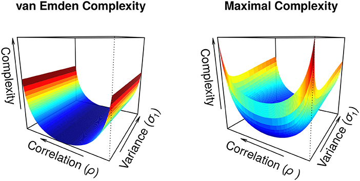
Figure 1. The van Emden complexity, C_vE(Σ), and maximal complexity, C_max(Σ), where $\Sigma =\left(\begin{array}{cc}{\sigma }_1^2& {\sigma }_1{\sigma }_2\rho \\ {\sigma }_1{\sigma }_2\rho & {\sigma }_2^2\end{array}\right)$ and σ₂ = 1.

In order to apply the penalties C_vE(Σ) and C_max(Σ) to real data we use the estimated covariance matrix, $\widehat{\Sigma }$. The parameter covariance matrix is extractable from the output of virtually all estimation packages. If parameters are estimated through direct optimization, optimization routines typically report an approximate Hessian. The inverse of the Hessian matrix is an approximation of the covariance matrix. Thus, ${\text{C}}_{\text{vE}}(\widehat{\Sigma })$ and ${\text{C}}_{\text{max}}(\widehat{\Sigma })$ can be easily calculated from output given by standard statistical packages such as R (R Core Team, 2015), which typically will report an approximate Hessian matrix that can be used to estimate the approximate covariance matrix by solving for the inverse of the matrix. For the small variance covariance matrices explored here solving for the inverse matrix is fast (less than 1 s) and the matrix would have to get quite large for the calculation time to be noticible, on the order of thousands of parameters. Other methods to estimate the covariance matrix such as using the least squares estimators or by bootstrapping estimates of the covariance matrix could also be applied.

ICC is not a scale-invariant penalty and transformations of the data may yield different model selections. Another form of ICC calculates the complexity penalty as a function of the correlation matrix, denoted as R, rather than of the covariance matrix (Bozdogan and Haughton, 1998). However, this quantity does not incorporate information about the precision of parameters estimates, as the variance terms are not present.

To overcome the limitations of the current form of scale-invariant ICC, we introduce a new variant based on a complexity measure that uses the coefficient of variation matrix (Boik and Shirvani, 2009). This matrix is independent of scale, but it retains information on the relative precision of the parameter estimates. The coefficient of variation matrix is defined as the covariance matrix scaled by the vector of parameter estimates in such a way that the diagonals are the squared coefficients of variation. This is a matrix with entries defined as ${\text{Ψ}}_{i,j}=\frac{\text{Cov}({\theta }_1,{\theta }_2)}{{\theta }_1{\theta }_2}$. Applying penalties of the form C_vE(Ψ) may be desirable because the matrix Ψ is invariant to multiplicatively rescaling the covariates but is still sensitive to the relative magnitude of coefficient uncertainty. Scale invariance means that going from one unit to another for a specific covariate, e.g., meters to kilometers, does not affect the inference. C_vE(Ψ) and C_max(Ψ) are sensitive to additive transformations, thus, shifting all measurement units by a constant factor will lead to different inferences. A table summarizing the properties of the different forms of informational complexity is given in Table 1.

TABLE 1

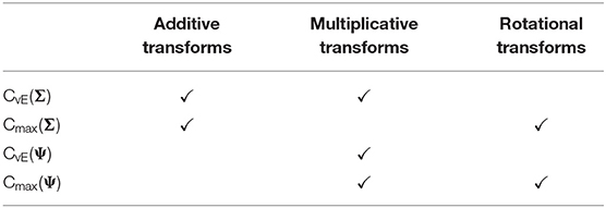
Table 1. Invariance of complexity forms to different linear transformations of the covariates.

2. Methods

2.1. Incorporating Parameter Estimability Into Information Criterion

The standard ICC does not penalize increasing complexity in a manner that leads to asymptotically consistent model selections (Nishii, 1988). Bozdogan and Haughton (1998) proposed a consistent form of the ICC that scaled the complexity parameter, C_max(Σ) by the log of the sample size, however this criterion did not perform well in their simulation experiments. Therefore, we propose a new compound selection criterion that is the sum of two divergences in order to develop a consistent form of criteria. The first divergence is a model parsimony measure. The second divergence, C₋(·), gives a measure of parameter estimability, a useful property for model interpretability and prediction. This criterion is defined as $\text{IC}+{\text{C}}_{-}(·)\equiv -2ln(L(\widehat{\theta }))+kf(n)+2{\text{C}}_{-}(·)$. The first piece of this criterion measures the goodness of fit through the maximum log-likelihood, the second piece measures model complexity, where f(n, k) is a function of the sample size and possibly of the number of parameters. The final piece, C₋(·), measures the parameter estimability. The exact form of this compound criterion depends on both the choice of the model parsimony criterion as well as the choice of the parameter complexity measure which regulates the strength of the penalty based on the complexity of the parameter.

Our motivation for using two divergences in this compound criterion is that we believe accounting for both goodness of fit and parameter estimability when using finite datasets will better reflect the underlying complexity and usefulness of the model. These compound criteria also deal with a critical issue in the ICC that yield a penalty of zero when parameters are orthogonal. Given that there are a number of measures of both goodness of fit and parameter complexity, we tested several different forms of the compound criterion. The forms we tested were AIC + 2C₋(·), AICc + 2C₋(·), BIC + 2C₋(·), and $\text{BI}{\text{C}}^{*}+2{\text{C}}_{-}(·)$ where C₋(·) can be ${\text{C}}_{\text{vE}}(\widehat{\Sigma })$, ${\text{C}}_{\text{vE}}(\widehat{\Psi })$, ${\text{C}}_{\text{max}}(\widehat{\Sigma })$, or ${\text{C}}_{\text{max}}(\widehat{\Psi })$.

2.2. Performance Comparisons With Simulation Studies

We conducted simulation studies that tested the capabilities of all 25 of the simple and compound information criteria discussed above under different conditions. We compared the behavior of model selection criteria using three attributes:

1. Selection: how frequently the criterion identifies the generating model.

2. Prediction: how well models selected by a criterion can predict new observations.

3. KL approximation: how well criterion values estimated KL divergence between model and truth.

The first two attributes reiterate the primary goals of model selection described in the introduction. The third attribute addresses the ability of a model to determine the relative KL divergence, a question of only collateral interest to practitioners interested in the application of model selection techniques to scientific problems. However, the estimated KL divergence may be a useful proxy for similarity to the generating model. In addition, much of the development and discussion of model identification criteria in ecology is framed around the estimation of the KL divergence as a metric between model and truth (for a review on other possible metrics see discussion in Lele, 2004).

We quantified attribute 1, the ability of a criterion to determine the generating model by counting the percentage of time that each criterion selected the generating model in our simulations. We measured attribute 2, a criterion's predictive ability, by its prediction sum of squares (PRESS) given by $\text{PRESS}={\displaystyle \sum _{i=1}^n{\left(y_i-{\widehat{y}}_{-i}\right)}^2}$. Here ŷ_−i is the predicted value at the i^th data point, which is omitted when fitting the model to the data, and y_i is the true, unobserved i^th value (Allen, 1974). A low PRESS value indicates that the criterion chooses a model that gives low prediction errors for in-sample prediction.

To calculate attribute 3, the frequency that criteria selected the minimum KL divergence between the j^th model and the generating distribution, we used the formula for the divergence between normal distributions (Bozdogan, 1987). We determined the agreement of each criterion with the true minimum KL divergence by calculating the frequency that the criterion selected the model with the minimum KL divergence.

To better understand the properties of these model selection criterion under a broad range of conditions we performed our simulation experiments with a set of linear models and two sets of nonlinear models of ecological interest. The linear model simulations varied the strength of correlation present in the design matrix as well as sample size and process variance. The first nonlinear model set examined time series models of population dynamics, while the second examined highly nonlinear models of barley yield. In both nonlinear model sets sample size and process variance were varied as well as the generating model. Using these different model sets, we sought to define criterion performance over the range of model complexity found in the ecological literature.

2.3. Linear Models

Our linear regression simulation experiment follows a design based on previous simulation studies by Bozdogan and Haughton (1998), Clark and Troskie (2006), and Yang and Bozdogan (2011). These studies explored the application of the ICC criterion under differing levels of correlation among explanatory variables. Correlation in explanatory variables is likely to be common in ecological covariates, causing the performance of the AIC to suffer (Bozdogan and Haughton, 1998).

We generated a 7 parameter design matrix by transforming 8 randomly drawn standard normal random variables, Z ~ N(0, 1), using the relationships:

$X_{i,j}=\{\begin{array}{l}\sqrt{1-{\alpha }_1^2}{Z}_{i,j}+{\alpha }_1{Z}_{i,8}\text{ for }j=1,2,3i=1,2,\dots ,n\hfill \\ \sqrt{1-{\alpha }_2^2}{Z}_{i,j}+{\alpha }_2{Z}_{i,8}\text{ for }j=4,5,6,7i=1,2,\dots ,n.\hfill \end{array}$

Where X_{i, j} is the ith entry of the jth covariate. The α₁ and α₂ values control the degree of correlation present among the elements of the design matrix. The covariates generated by using this procedure have a covariance between row j and row k given by,

$\text{Cov}(X_j,X_k)=\{\begin{array}{l}{\alpha }_1^2\text{ for }j=1,2,3,k=1,2,3\hfill \\ {\alpha }_2^2\text{ for }j=4,5,6,7,k=4,5,6,7\hfill \\ {\alpha }_1{\alpha }_2\text{ for }j=1,2,3,k=4,5,6,7.\hfill \end{array}$

The covariate parameters, β, were generated from the maximum eigenvector of the matrix X′X following Bozdogan and Haughton (1998).

We generated data at three different levels of collinearity, low (α₁ = 0.3, α₂ = 0.7), medium (α₁ = 0.9, α₂ = 0.9), and high (α₁ = 0.99, α₂ = 0.99); three levels of sample size, low (n = 20), medium (n = 50), and high (n = 100); and three levels of variability, low (σ² = 0.25), medium (σ² = 1), and high (σ² = 2.5). We simulated 100 datasets from the rank 5 model at each level of collinearity, sample size, and variance. We then repeated each set of 100 simulations 10 times to estimate a mean and standard error of each selection attribute.

We then fit all models of ranks (1–7) to the generated data using the BFGS algorithm in the optim routine in the R statistical language. Hessian matrices were calculated using the Hessian function in the numDeriv package (Gilbert and Varadhan, 2016). We checked convergence of the optimization by checking that all eigenvalues of the Hessian matrix were positive. For each simulated dataset we calculate the information criteria of each fitted model and determined how well the criteria performed in our three selection attributes.

We determined performance at each level of collinearity, sample size, and variance by averaging the statistic of interest (e.g., the number of correct generating model selections) over all of the simulation study parameters except the level of interest. For example, to determine performance at the low collinearity level we averaged the performance statistic of interest over all sample sizes and variances that had design matrices with low collinearity.

2.4. Population Dynamics Models

Dynamical time series models are a common applied modeling technique for forecasting future ecological conditions, a major goal of ecological modeling (Clark et al., 2001). Applications of time series models include forecasting fisheries stocks (Lindegren et al., 2010) and assessing extinction risk (Ferguson and Ponciano, 2014). Measuring the strength of evidence among a set of forecast models is critical for generating reliable predictions, but it's known that many nonlinear dynamical models yield correlated parameter estimates (Polansky et al., 2009). These correlations may impact the performance of traditional information criterion (Bozdogan, 1990). Here, we study the properties of information criterion in a set of nonlinear dynamical models.

The population dynamics simulation experiment used time series models to describe the projected population abundance in the next year given the abundance in the current year. In order to ensure that population dynamics were realistic, we generated data based on parameter estimates made from the Global Population Dynamics Database (GPDD) to simulate data (NERC, 2010). The GPDD contains approximately 5000 time series related to plant and animal index measurements. We used a subset of these studies, chosen for their length and the indicated data quality following the methods described in more detail in Ferguson and Ponciano (2015) and Ferguson et al. (2016). We only used time series with a length of at least 15 samples and a GPDD reliability rating of 3–5. The reliability rating is a qualitative measure of data quality made by the database authors. These quality standards left us with 391 time series to generate data from.

We examined six density-dependent models encompassing a wide range of functional forms. All models were of the form, N_t+1 = rN_tf(N_t) where f(N_t) can take one of the commonly used functional forms of density dependence given in Table 2. These functional forms represent different hypotheses about the strength of density dependence. As in the linear model design, we examined a range of sample sizes (n = 25, n = 50, n = 100) and low, medium, and high process variances (see below for how we calculated these variances).

TABLE 2

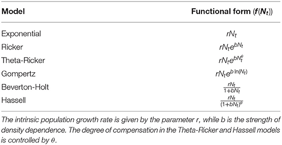
Table 2. Forms of density dependence used in the population dynamics study.

In order to determine realistic levels of variance to use in our simulations, we fit an additive, normally distributed environmental variance model to the population growth rate (pgr), where $\text{pgr}=ln\left(\frac{N_{t+1}}{N_t}\right)$. To determine realistic levels of environmental variation, we fit the pgr to a linear model (corresponding to Gompertz density dependence in Table 2) for all 391 time series. Optimization and convergence checks were performed on the pgr using the same methods described in the linear model section. We then used the 10, 50, and 90% quartiles of the estimated environmental variance over all time series to determine the low, medium, and high variance levels used in the simulations.

To simulate data, we first fit each of the density dependence model to each of the 391 GPDD datasets. We then simulated a new dataset from each fitted model at each level of sample size and variance, repeating this process for all of the density dependence models in Table 2. We repeated this process for every possible generating model, sample size, and variance combination, repeating the whole procedure 10 times to obtain a standard error for the model selection attributes. We averaged criteria performance over sample size, variance level, and generating model to examine the average selection rate for a given factor of interest. We did not need to vary the correlations between parameters in this experiment as in the linear models because the nonlinear model structure induces correlations between parameters.

2.5. Barley Yield Models

Bioeconomic modeling is an increasingly important application of ecological modeling (Grafton et al., 2017). Here, we examined the selection properties information criterion applied to a set of crop-weed competition models. These models explain crop yield (Y) as a function of crop (D_c) and weed (D_w) density, as well as the relative difference in time to emergence (T) between crop and weed. Here we examined our ability to accurately select the correct barley yield model from a set of candidate models. The nine models considered for this simulation experiment are a subset from a previous study (Jasieniuk et al., 2008) that used the ICC. These models have more complex forms than the population dynamics models used above, as well as more parameters and more covariates. Thus, this model set is a step up in complexity from the population dynamics models explored in the previous section. The nine models used in this simulation study are defined in Table 3. We refer readers to the original study by Jasieniuk et al. (2008) for further motivation for these models.

TABLE 3

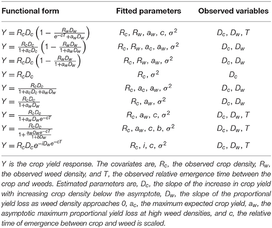
Table 3. Functional forms of the models used for the barley yield simulations.

We generated datasets by first fitting each of the models to the dataset from the Bozeman 1994 dataset reported in Jasieniuk et al. (2008). We simulated new datasets by adding a normal random noise term to the log of the empirically predicted response using data from Jasieniuk et al. (2008). We examined three sample size levels (n = 25, n = 50, n = 125) and three variance levels $({\sigma }^2=0.5{\widehat{\sigma }}^2,{\sigma }^2={\widehat{\sigma }}^2,{\sigma }^2=4{\widehat{\sigma }}^2)$, where ${\widehat{\sigma }}^2$ was the empirically estimated variance of the observed data under the given generating model. We generated 100 simulated datasets for each model in Table 3 at each sample size and variance level. As before, we averaged over sample size, variance level, and generating model to examine the average selection rate for a given factor of interest. We repeated each set of simulations 10 times to order to estimate the mean and standard error of the selection statistics. We only performed the PRESS calculation on one set of simulations due to the length of time it took to do this calculation. Therefore, there is no standard error associated with prediction for these models.

Due to these models presenting a more difficult optimization problem than the other model sets, we modified our fitting procedure. From an initial set of parameters, we applied the Nelder-Mead optimization algorithm (also known as the downhill simplex method) followed by the BFGS method to maximize the log-likelihood function. The simplex method was run first because it is robust, although it converges slowly. This two-step process provided the initial parameter estimates for the quasi-Newton method, which converges relatively quickly near a maximum. We repeated this procedure for 100 random initial points and chose the parameters associated with the maximum likelihood value, and convergence was determined as previously described.

3. Results

Here, we will focus on presenting the criteria that performed best under one or more of our experimental conditions. Figures of performance for all criterion under all experimental conditions are presented in the Supplementary Material.

3.1. Linear Models

We present the overall criterion performance averaged over all conditions, along with standard errors for the linear model simulations in Figure 2. The best criterion at selecting the generating model on average was the AICc (Table 4), the best at prediction was also the AICc (Table 5), and the best at selecting the minimum KL divergence was AICc+2C_max(Σ) (Table 6). The ICC tended to be the worst performers at all selection goals (Figure 2), however the ICC_max(Ψ) tended to behave similarly to the AIC and the BIC*. We also see in Figure 2 that the average performance of the criterion for all selection goals was strongly correlated but the PRESS and KL minimum selection was nearly completely correlated. Several of the compound criteria performed well with AICc+2C_max(Σ), AICc + 2C_vE(Σ), and AICc + 2C_vE(Ψ) performing nearly as well as AICc for all performance attributes.

FIGURE 2

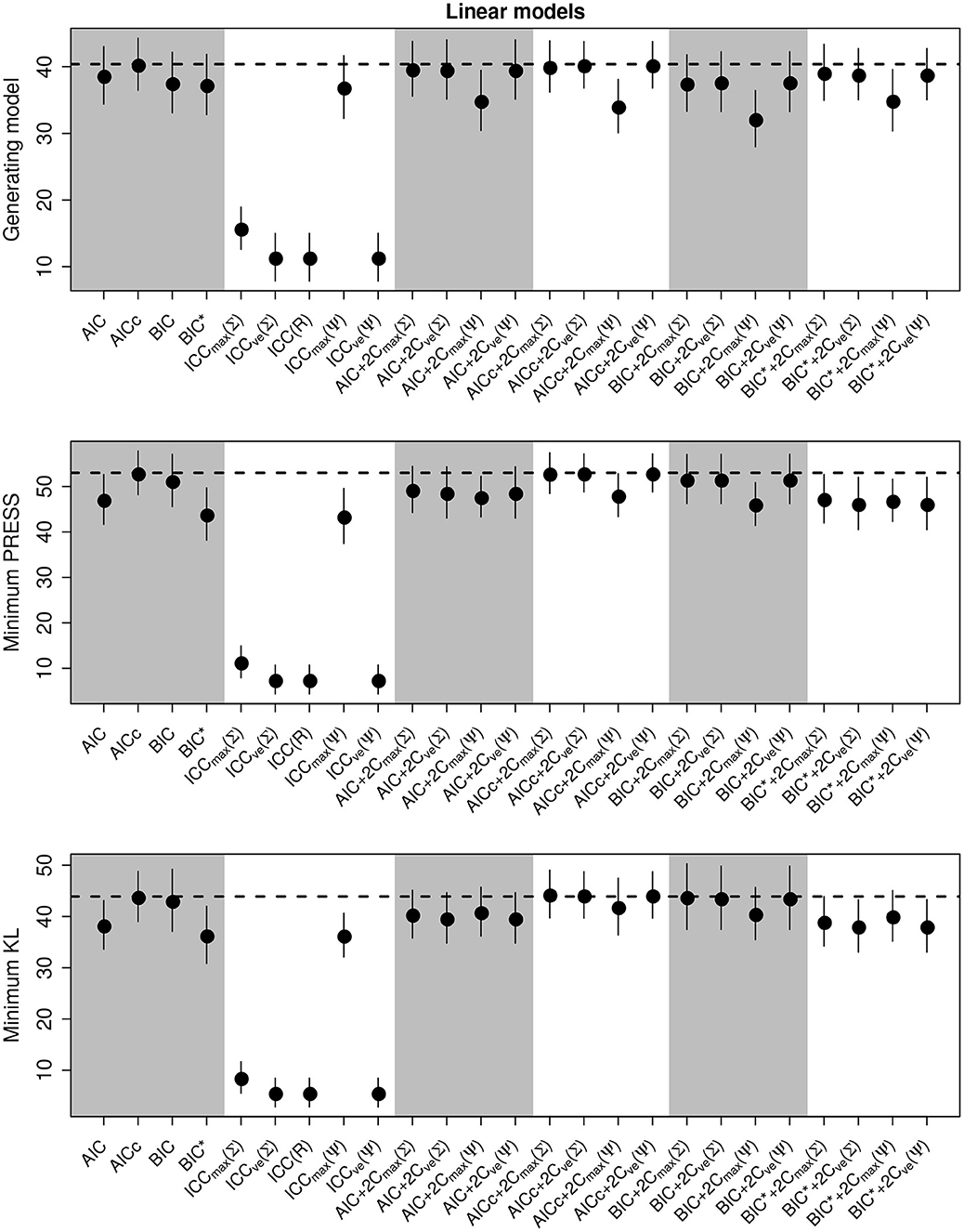
Figure 2. Performance of the criterion for all selection goals for the linear model simulation experiment. Points are the average performance-level, bars give standard errors. The dashed horizontal line gives the performance of AICc for reference. The top panel gives the frequency that each criterion selects the model used to generate the data, the middle pannel gives the frequency of selecting the model that minimizes the predicted residual error sum of squares (PRESS), while the bottom panel gives the frequency of selection by the criterion of the model corresponding to the minimum Kullback-Leibler divergence (KL).

TABLE 4

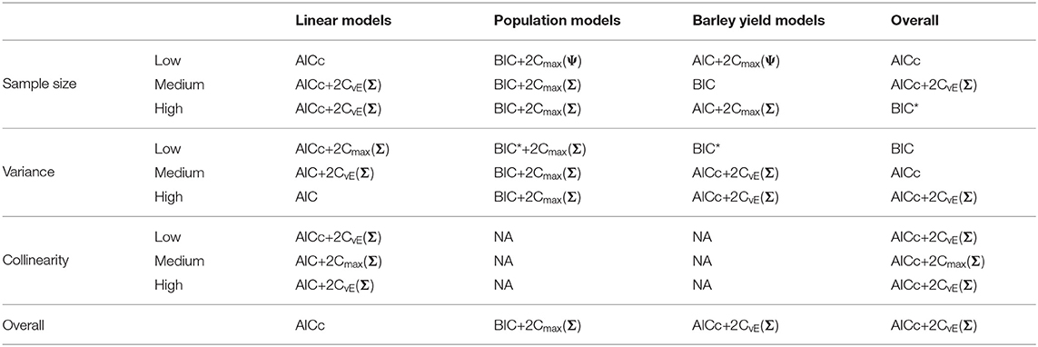
Table 4. Best performing information criteria at selecting the generating model from the candidate set.

TABLE 5

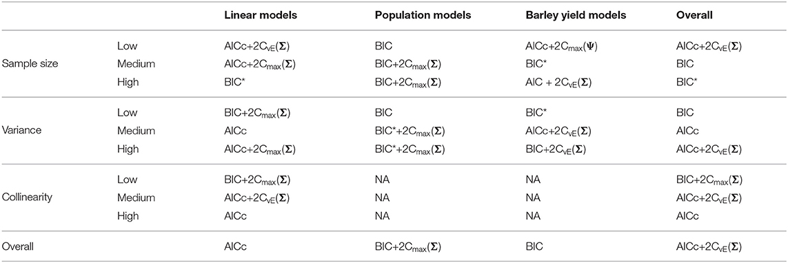
Table 5. Best performing information criteria at selecting the optimal predictive model from the candidate set.

TABLE 6

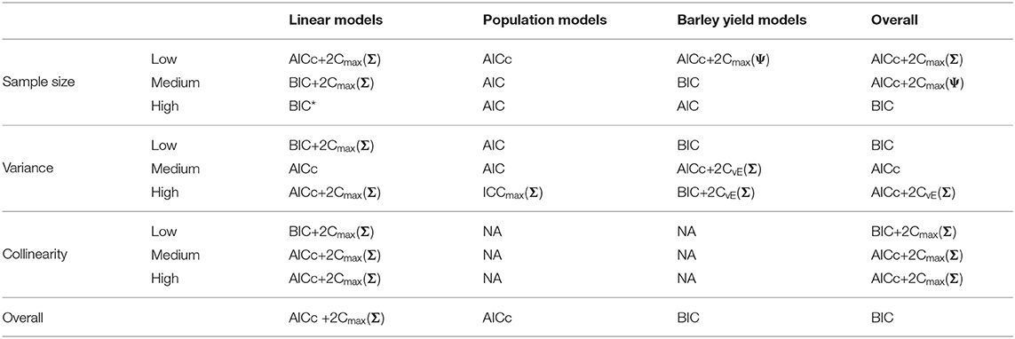
Table 6. Best performing information criteria at selecting the minimum KL divergence from the candidate set.

In general, criteria performed better as sample size increased and variance decreased as expected (Supplementary Figures S1–S6). In most trials some form of the compound criterion performed better than traditional criterion (Figure 2). However, performance differences among most of the criteria differed only by a few percentage points and the difference in top performers was within the range of the performance uncertainty (Figure 2).

3.2. Population Dynamics Models

We present the overall criterion performance for the population dynamics simulation experiments averaged over all conditions, along with standard errors, in Figure 3. While the class of ICC criteria performed poorly in the linear model selections, here they tended to perform as well as or better than the traditional criteria. While the performance of all selection goals in the linear models simulations were strongly correlated, here they differed. The variation in the performance of the ability to select the generating model was much greater than for the other selection goals, though the compound criteria did tend to perform better than both traditional criteria and the ICC.

FIGURE 3

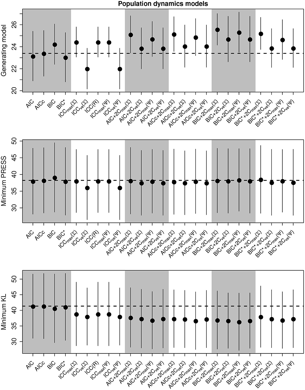
Figure 3. Performance of the criterion for all selection goals for the nonlinear population dynamics model simulation experiment. Points are the average performance-level, bars give standard errors. The top panel gives the frequency that each criterion selects the model used to generate the data, the middle pannel gives the frequency of selecting the model that minimizes the predicted residual error sum of squares (PRESS), while the bottom panel gives the frequency of selection by the criterion of the model corresponding to the minimum Kullback-Leibler divergence (KL).

Out of the ICC the ICC_max(Ψ) tended to perform as good as, or better than the other forms. The best criterion at selecting the generating model overall was the BIC+2C_max(Σ) (Table 4), the best at prediction was the BIC+2C_max(Σ) (Table 5), and the best at selecting the minimum KL divergence was the AICc (Table 6).

In general, criteria performed better at selecting the generating model and the KL minimum as sample size increased and variance decreased, as expected, however, the ability to select the minimum PRESS model actually declined in the traditional criteria with sample size (Supplementary Figures S7–S12). Additionally, we found that some form of the compound criterion tended to perform better than the traditional criterion for all selection goals with BIC+2C_max(Σ) performing best at selecting the generating model the best predictive model. However, the AIC and AICc tended to dominate the performance of the KL divergence selection. Performance differences among most of the criteria differed only by a few percentage points and the difference between top performers was within the range of the performance uncertainty (Figure 3).

3.3. Barley Yield Models

We present the overall criterion performance for the barley yield model simulation experiments, along with standard errors, in Figure 4. While the performance of criteria was strongly correlated across all selection goals in the linear models, here performance was not correlated. While the selection of the minimum KL divergence was highly variable, similar to the population dynamics models, the PRESS performance was very consistent between criterion. Here, the class of ICC criteria tended to perform poorly though ICC_max(Ψ) again tended to be consistent with the standard criterion and to perform better than the other forms of ICC (Figure 3). The compound criterion tended to perform better than the standard criterion but tended to perform worse at selecting the generating model.

FIGURE 4

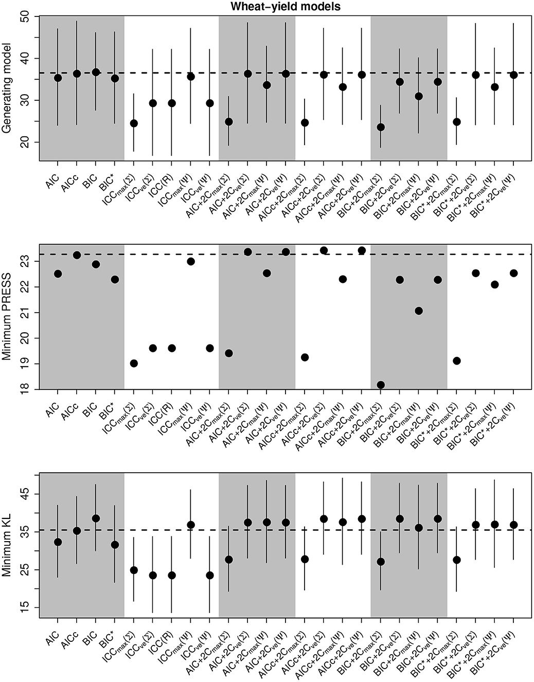
Figure 4. Performance of the criterion for all selection goals for the nonlinear barley yield simulation experiment. Points are the average performance-level, bars give standard errors. The top panel gives the frequency that each criterion selects the model used to generate the data, the middle pannel gives the frequency of selecting the model that minimizes the predicted residual error sum of squares (PRESS), while the bottom panel gives the frequency of selection by the criterion of the model corresponding to the minimum Kullback-Leibler divergence (KL). No error bars are present in the PRESS results becauase we did not repeat these experiments.

Overall, the best criterion at selecting the generating model on average was the AICc+2C_vE(Σ), while the best at prediction and at selecting the minimum KL divergence was the BIC (Table 6). In general, criteria performed better as sample size increased and variance decreased for selecting the generating model and the KL minimum, as expected (Supplementary Figures S13–S18). Performance differences among most of the criteria differed only by a few percentage points and the difference in top performers was within the range of performance uncertainty (Figure 4).

Finally, we found that overall performance across all simulations varied by the selection goals. The best at selecting both the generating model and the best predictive model overall was AICc+2C_vE(Σ) (Tables 4, 5). The criterion that performed best at selecting the KL minimum was BIC (Table 6).

4. Discussion

The compound criterion AICc+2C_vE(Σ) performed best on average at selecting both the generating model and the best predictive model, two important goals of ecological modeling. Surprisingly, the BIC performed best at selecting the model corresponding to the minimum KL divergence even though it is not meant to be an estimate of this quantity. Although the KL divergence is not a quantity that is itself of interest to scientists, it may be useful as a measure of the distance to truth. Despite the strong overall performance of the compound criteria, differences in performance between the top criteria were small. For example, while AICc+2C_vE(Σ) performed best and selected the generating model 33.1% of the time across all experimental conditions, AICc selected the generating model 32.1% of the time and BIC selected the generating model 31.0% of the time.

Previous studies have looked at the performance of the ICC on linear regression models (Bozdogan, 1990; Bozdogan and Haughton, 1998; Clark and Troskie, 2006; Yang and Bozdogan, 2011), mixture models (Windham and Cutler, 1992; Bozdogan, 1993; Miloslavsky and Laan, 2003) and time series models (Bozdogan, 2000; Clark and Troskie, 2008). This past work has generally found much better performance of the ICC's than our study. For example, linear regression simulations suggest that the criteria may often outperform AIC and BIC, though limitations in study design are likely responsible for the different results. Two of these studies on linear regression (Bozdogan and Haughton, 1998; Clark and Troskie, 2006) did not allow for overfitting the generating model. While a third study (Yang and Bozdogan, 2011) did include the potential for overfitting, the variation in the extra model covariates were two orders of magnitude larger than the covariates of the generating model. This may not provide a realistic assessment of performance, as practitioners are often interested in distinguishing between effects that vary on the same scale. The results of the time series model application of ICC appeared more promising as ICC tended to do better than AIC or BIC most of the time when selecting among autoregressive moving average models (Clark and Troskie, 2008). Our population dynamics simulations also suggest that the ICC criteria perform better at selecting the generating model in nonlinear time series analysis than in linear regression, however we found that performance of the ICC criterion was rarely a significant improvement over AICc.

While many of the ICC performed poorly in our simulation experiments, the newly developed ICC_max(Ψ) was comparable to the traditional criterion for all selection goals. ICC_max(Ψ) uses the coefficient of variation matrix, accounting for uncertainty in parameter estimation. The compound criteria tended to provide superior performance over the other ICC measures. Even though the ICC_max(Ψ) performed well as a criterion on its own, when incorporated as a compound criterion it tended to slightly underperform the best compound criteria. This is likely because the penalty term of the compound criteria ended up being too severe. Further work designed to optimize the weighting of the components might improve the performance of the compound criteria.

In the linear model simulation experiment, the AICc tended to do better than the BIC at selecting the generating model (Figure S1). In contrast, our population dynamics and barley yield simulation experiments found that BIC outperformed the AICc at selecting the generating model (Figures S7, S13). These results are broadly consistent with guidelines developed by Burnham and Anderson (2004) who outline how the BIC can be expected to outperform AIC when there are a few large effects. In systems with many small effects, such as the one used in our linear model experiments, the AIC will be expected to perform best. Further work by Brewer et al. (2016) has highlighted that the presence of multicollinearity can reverse these recommendations, with BIC generally selecting select better predictive models than the AIC. A previous study on population models by Corani and Gatto (2007) found that AICc outperformed BIC; however, this study was on nested models so the scenario more closely resembled our linear model simulation experiment. In a study design similar to our own, Hooten (1995) found that the BIC did better than either the AIC or the AICc at selecting the form of the generating model when selecting among density dependence forms, consistent with our results.

Averaging over all experimental factors provides a useful metric for assessing the general performance in complex ecological models. However, performance was highly variable on specific simulation experiments and even among experimental factors. We ascribe the differences between our results, which found only modest differences among criteria, and previous work to the broad array of simulation conditions. Averaging across these conditions provides a better guide to how criterion perform under a range of scenarios, though at the cost of providing less guidance for specific modeling scenarios. As Forster (2000) points out the performance of any criterion is context dependent and criteria will have a domain where they may be superior and where they may be inferior.

Designers and consumers of simulation validation studies need to carefully consider if performance is being assessed in a domain relevant to their modeling objectives. One potential approach to deal with the variability in performance is to conduct simulation experiments for every particular study to determine the optimal criterion. We would caution against this, besides performance being conditional on the particular model set, we expect this would lead to an anthology of idiosyncratic selection methodologies. Instead, we advise practitioners to rely on a criterion that has been shown to be consistent with their modeling goals and effective in a wide range of scenarios. Finally, there is no automated model selection approach that will substitute the clear-headed thinking that necessary to develop distinct, testable hypotheses that will answer the scientific question at hand. When this clarity is not possible, it may be preferable to develop a single, comprehensive model rather than performing model selection.

Our compound criteria are the sum of two estimated divergences. The first divergence attempts to measure the discrepancy between the model and truth. This model discrepancy can be estimated by AIC, AICc, BIC, BIC*, or one of the many other existing criteria. The second divergence estimates the distance between the joint sampling distribution of the parameters and the product of the marginal sampling distributions of the parameters. The motivation behind including this second divergence is to assess the estimability of parameters, a model quality that is often overlooked but has important implications when interpreting estimates, making out-of-sample predictions, and transferring parameters and models for use in other contexts. Thus, this divergence is a measure of a models usefulness. Our results suggest compound criterion that balance traditional measures of fit and complexity with an additional measure of usefulness can improve ecological inference. We found the AICc+2C_vE(Σ) to be the best combination of these terms out of those considered here for both selecting the generating model and for prediction. AICc likely performed well because even the largest sample sizes explored here were relatively low, a common issue in many ecological datasets.

For the informational complexity we used a measure developed in past work based on the KL divergence between the joint and marginal sampling distributions of parameter estimates (van Emden, 1969; Bozdogan, 2000) (Equation 3). While the KL divergence has taken a primary role in ecological model selection, it is a divergence not a true distance. This means that the KL divergence between the distributions f and g is not necessarily equal to the KL divergence between g and f. In contrast, the Hellinger and Bhattacharyya distances are both true distance measures and have this symmetry property. Using an alternative measure may improve interpretability of the informational complexity, however it is not clear that these quantities have the same informational interpretation as the KL divergence, therefore it is not clear how to best combine these distance measures with information criterion.

Bozdogan and Haughton (1998) developed a consistent form of ICC by scaling the complexity measure, C_max(Σ) by ln(n). While this does yield a consistent criterion, the performance of this ad-hoc approach was poor in their simulation studies. Our own preference is to use a compound criterion with a consistent form such as BIC. This study shows that BIC+2C_vE(Ψ) achieves all measures of quality well under a broad range of modeling frameworks and it has the theoretical advantage of being scale invariant and consistent. Furthermore, the BIC is consistent at large sample size. At small sample size the BIC tends to choose compact model where all of the model components are well supported. Leading, we think, to a greater ease of interpretation (e.g., Arnold, 2010; Leroux, 2019).

While our analysis only considers a single best model, there are often likely to be several models that perform nearly as well due to the flexibility of the models in our simulation designs. Bayesian model averaging, and the complementary model averaging approach developed using AIC (Burnham and Anderson, 2002), is one common approach to account for uncertainty in model selection (but see Ponciano and Taper, submitted this issue). Model averaging can provide more precise parameter estimates (e.g., Vardanyan et al., 2011) and ensemble predictions can be more accurate than a single model (e.g., Martre et al., 2015). Given that our compound criterion performed slightly better than the standard information criterion for in-sample prediction and provides a measure of parameter dependence we expect that the compound criteria are suitable for model averaging and may directly address one major criticism of model averaging, the necessity of covariate independence (Cade, 2015).

We have assumed an equal weighting of the divergence between model and truth and the divergence measuring parameter complexity, though we could also choose to weight these contributions differently. One approach would be to calculate the optimal weights using simulation methods, while another approach is to allow the researcher to apply a priori weights based on the value a researcher places on model parsimony and estimability. It is these epistemic considerations that served as inspiration for developing these compound criteria so such a weighting would be consistent our original motivation.

This study provides evidence that developing information criterion based on measures other than the divergence between model and truth can yield improved model selection performance. However, we found that differences in performance between the best compound criterion and standard criteria were often small. This result aligns with previous work (Murtaugh, 2009) suggesting that standard methods tend to consistently produce models that are statistically and scientifically useful, though not necessarily optimal. Given that standard criteria are typically easy to calculate from regression output they provide useful and reliable tools for practicing ecologists. The compound criteria here can also be calculated from standard output suggesting that they could also be widely applied. Computational procedures such as regression trees (Murtaugh, 2009) or statistical learning methods (Corani and Gatto, 2006a,b, 2007) may also be useful tools under a wide variety of conditions, however these methods can be time demanding. The compound criteria examined here yield improved performance of model selection without dramatically increasing the amount of work needed to do inference.

Data Availability Statement

Publicly available datasets were analyzed in this study. This data can be found here: https://www.imperial.ac.uk/cpb/gpdd2/secure/login.aspx.

Author Contributions

MT and JF conceived of the presented ideas. JF developed the theory and implemented the simulations. RZ-F, MT, MJ, and BM verified the analyses. MJ developed the suite of yield models. All authors discussed the results and contributed to the final manuscript.

Funding

MT has been supported in part by MTFWP contract #060327 while JF and BM were supported in part by USDA NRI Weedy and Invasive Plants Program Grant No. 00-35320-9464.

Conflict of Interest

The authors declare that the research was conducted in the absence of any commercial or financial relationships that could be construed as a potential conflict of interest.

Acknowledgments

We thank R. Boik, Mark Greenwood, Steve Cherry, Subhash Lele, Jose Ponciano, Taal Levi, Kristen Sauby, and Robert Holt for comments on earlier drafts of this work. MT's understanding of the problem of model identification has been greatly enhanced over the years by discussions with Subhash Lele, Brian Dennis, and Jose Ponciano.

Supplementary Material

The Supplementary Material for this article can be found online at: https://www.frontiersin.org/articles/10.3389/fevo.2019.00427/full#supplementary-material

References

Aho, K., Derryberry, D., and Peterson, T. (2014). Model selection for ecologists: the worldviews of AIC and BIC. Ecology 95, 631–636. doi: 10.1890/13-1452.1

PubMed Abstract | CrossRef Full Text | Google Scholar

Akaike, H. (1974). A new look at the statistical model identification. IEEE Trans. Automat. Contr. 19, 716–723. doi: 10.1109/TAC.1974.1100705

CrossRef Full Text

Allen, D. (1974). The relationship between variable selection and data agumentation and a method for prediction. Technometrics 16, 125–127. doi: 10.1080/00401706.1974.10489157

CrossRef Full Text | Google Scholar

Arnold, T. W. (2010). Uninformative parameters and model selection using Akaike's information criterion. J. Wildl. Manage 74, 1175–1178. doi: 10.1111/j.1937-2817.2010.tb01236.x

CrossRef Full Text | Google Scholar

Boik, R., and Shirvani, A. (2009). Principal components on coefficient of variation matrices. Stat. Methodol. 6, 21–46. doi: 10.1016/j.stamet.2008.02.006

CrossRef Full Text | Google Scholar

Bozdogan, H. (1987). Model selection and Akaike's information criterion (AIC): the general theory and its analytical extensions. Psychometrika 52, 345–370. doi: 10.1007/BF02294361

CrossRef Full Text | Google Scholar

Bozdogan, H. (1990). On the information-based measure of covariance complexity and its application to the evaluation of multivariate linear models. Commun. Stat. A Theor. 19, 221–278. doi: 10.1080/03610929008830199

CrossRef Full Text | Google Scholar

Bozdogan, H. (1993). “Choosing the number of component clusters in the mixture-model using a new informational complexity criterion of the inverse-Fisher information matrix,” in Information and Classification (Berlin; Heidelberg: Springer), 40–54.

Google Scholar

Bozdogan, H. (2000). Akaike's information criterion and recent developments in information complexity. J. Math. Psychol. 44, 62–91. doi: 10.1006/jmps.1999.1277

PubMed Abstract | CrossRef Full Text | Google Scholar

Bozdogan, H., and Haughton, D. (1998). Informational complexity criteria for regression models. Comput. Stat. Data Anal. 28, 51–76. doi: 10.1016/S0167-9473(98)00025-5

CrossRef Full Text | Google Scholar

Brewer, M. J., Butler, A., and Cooksley, S. L. (2016). The relative performance of AIC, AICCand BIC in the presence of unobserved heterogeneity. Methods Ecol. Evol. 7, 679–692. doi: 10.1111/2041-210X.12541

CrossRef Full Text | Google Scholar

Brun, R., Reichert, P., and Künsch, H. R. (2001). Practical identifiability analysis of large environmental simulation models. Water Resour. Res. 37, 1015–1030. doi: 10.1029/2000WR900350

CrossRef Full Text | Google Scholar

Burnham, K. K. P., and Anderson, D. D. R. (2004). Multimodel inference: understanding AIC and BIC in model selection. Sociol. Method Res. 33, 261–304. doi: 10.1177/0049124104268644

CrossRef Full Text | Google Scholar

Burnham, K. P., and Anderson, D. R. (2002). Model Selection and Multimodel Inference: A Practical Information-theoretic Approach. New York, NY: Springer-Verlag.

Cade, B. S. (2015). Model averaging and muddled multimodel inferences. Ecology 96, 2370–2382. doi: 10.1890/14-1639.1

PubMed Abstract | CrossRef Full Text | Google Scholar

Cavanaugh, J. (1997). Unifying the derivations for the Akaike and corrected Akaike information criteria. Stat. Probabil. Lett. 33, 201–208. doi: 10.1016/S0167-7152(96)00128-9

CrossRef Full Text | Google Scholar

Clark, A. E., and Troskie, C. G. (2006). Regression and ICOMP-A simulation study. Commun. Stat. B Simul. 35, 591–603. doi: 10.1080/03610910600716910

CrossRef Full Text | Google Scholar

Clark, A. E., and Troskie, C. G. (2008). Time series and model selection. Commun. Stat. B Simul. 37, 766–771. doi: 10.1080/03610910701884153

CrossRef Full Text | Google Scholar

Clark, J. S., Carpenter, S. R., Barber, M., Collins, S., Dobson, A., Foley, J., et al. (2001). Ecological forecasts: an emerging imperative. Science 293, 657–660. doi: 10.1126/science.293.5530.657

PubMed Abstract | CrossRef Full Text | Google Scholar

Corani, G., and Gatto, M. (2006a). Model selection in demographic time series using VC-bounds. Ecol. Model 191, 186–195. doi: 10.1016/j.ecolmodel.2005.08.019

CrossRef Full Text | Google Scholar

Corani, G., and Gatto, M. (2006b). VC-dimension and structural risk minimization for the analysis of nonlinear ecological models. Apple Math. Comput. 176, 166–176. doi: 10.1016/j.amc.2005.09.050

CrossRef Full Text | Google Scholar

Corani, G., and Gatto, M. (2007). Erratum selection in demographic time series using VC-bounds. Ecol. Model 200, 273–274. doi: 10.1016/j.ecolmodel.2006.08.006

CrossRef Full Text | Google Scholar

Cox, D. (1990). Role of models in statistical analysis. Stat. Sci. 5, 169–174. doi: 10.1214/ss/1177012165

CrossRef Full Text | Google Scholar

Dietze, M. C., Fox, A., Beck-johnson, L. M., Betancourt, J. L., Hooten, M. B., Jarnevich, C. S., et al. (2018). Iterative near-term ecological forecasting: needs, opportunities, and challenges. Proc. Natl. Acad. Sci. U.S.A. 115, 1424–1432. doi: 10.1073/pnas.1710231115

PubMed Abstract | CrossRef Full Text | Google Scholar

Dormann, C. F., Elith, J., Bacher, S., Buchmann, C., Carl, G., Carré, G., et al. (2013). Collinearity: a review of methods to deal with it and a simulation study evaluating their performance. Ecography 36, 27–46. doi: 10.1111/j.1600-0587.2012.07348.x

CrossRef Full Text | Google Scholar

Ferguson, J. M., Carvalho, F., Murillo-García, O., Taper, M. L., and Ponciano, J. M. (2016). An updated perspective on the role of environmental autocorrelation in animal populations. Theor. Ecol. 9, 129–148. doi: 10.1007/s12080-015-0276-6

PubMed Abstract | CrossRef Full Text | Google Scholar

Ferguson, J. M., and Ponciano, J. M. (2014). Predicting the process of extinction in experimental microcosms and accounting for interspecific interactions in single-species time series. Ecol. Lett. 17, 251–259. doi: 10.1111/ele.12227

PubMed Abstract | CrossRef Full Text | Google Scholar

Ferguson, J. M., and Ponciano, J. M. (2015). Evidence and implications of higher-order scaling in the environmental variation of animal population growth. Proc. Natl. Acad. Sci. U.S.A. 112, 2782–2787. doi: 10.1073/pnas.1416538112

PubMed Abstract | CrossRef Full Text | Google Scholar

Ferguson, J. M., Taper, M. L., Guy, C. S., and Syslo, J. M. (2012). Mechanisms of coexistence between native bull trout (Salvelinus confluentus) and non-native lake trout (Salvelinus namaycush): inferences from pattern-oriented modeling. Can. J. Fish. Aquat. Sci. 769, 755–769. doi: 10.1139/f2011-177

CrossRef Full Text | Google Scholar

Forster, M. (2000). Key concepts in model selection: performance and generalizability. J. Math. Psychol. 44, 205–231. doi: 10.1006/jmps.1999.1284

PubMed Abstract | CrossRef Full Text | Google Scholar

Freckleton, R. P. (2011). Dealing with collinearity in behavioural and ecological data: model averaging and the problems of measurement error. Behav. Ecol. Sociobiol. 65, 91–101. doi: 10.1007/s00265-010-1045-6

CrossRef Full Text | Google Scholar

Giere, R. N. (2004). How models are used to represent reality. Philos. Sci. 71, 742–752. doi: 10.1086/425063

CrossRef Full Text | Google Scholar

Gilbert, P., and Varadhan, R. (2016). numDeriv: Accurate Numerical Derivatives. R package version 2016.8-1. Available online at: https://CRAN.R-project.org/package=numDeriv

Grafton, R. Q., Kirkley, J., and Squires, D. (2017). Economics for Fisheries Management. New York, NY: Routledge.

Google Scholar

Haughton, D. M. A. (1988). On the choice of a model to fit data from an exponential family. Ann. Stat. 16, 342–355. doi: 10.1214/aos/1176350709

CrossRef Full Text | Google Scholar

Hooten, M. (1995). Distinguishing forms of statistical density dependence and independence in animal time series data using information criteria. (Ph.D. thesis). Montana State University, Bozeman, MT, United States.

Google Scholar

Hurvich, C. M., and Tsai, C.-L. L. (1989). Regression and time series model selection in small samples. Biometrika 76, 297–307. doi: 10.1093/biomet/76.2.297

CrossRef Full Text | Google Scholar

Jasieniuk, M., Taper, M. L., Wagner, N. C., Stougaard, R. N., Brelsford, M., and Maxwell, B. D. (2008). Selection of a barley yield model using information-theoretic criteria. Weed Sci. 56, 628–636. doi: 10.1614/WS-07-177.1

CrossRef Full Text | Google Scholar

Lele, S. R. (2004). “Error functions and the optimality of the law of likelihood,” in The Nature of Scientific Evidence: Statistical, Philosophical and Empirical Considerations, eds M. L. Taper and S. R. Lele (Chicago, IL: The University of Chicago Press), 191–203.

Google Scholar

Lele, S. R., and Taper, M. L. (2012). “Information criteria in ecology,” in Encyclopedia of Theoretical Ecology, eds A. Hastings and L. Gross (Berkeley, CA: University of California Press), 371–376.

Leroux, S. J. (2019). On the prevalence of uninformative parameters in statistical models applying model selection in applied ecology. PLoS ONE 14:e0206711. doi: 10.1371/journal.pone.0206711

PubMed Abstract | CrossRef Full Text | Google Scholar

Lindegren, M., Mollmann, C., Nielsen, A., Brander, K., Mackenzie, B. R., and Stenseth, N. C. (2010). Ecological forecasting under climate change : the case of Baltic cod. Proc. R. Soc. B Biol. Sci. 277, 2121–2130. doi: 10.1098/rspb.2010.0353

PubMed Abstract | CrossRef Full Text | Google Scholar

Link, W. A., and Sauer, J. R. (2016). Bayesian cross-validation for model evaluation and selection, with application to the North American breeding survey. Ecology 97, 1746–1758. doi: 10.1890/15-1286.1

PubMed Abstract | CrossRef Full Text | Google Scholar

Link, W. A., Sauer, J. R., and Niven, D. K. (2017). Model selection for the North American Breeding Bird Survey: a comparison of methods. Condor 119, 546–556. doi: 10.1650/CONDOR-17-1.1

CrossRef Full Text | Google Scholar

Martre, P., Wallach, D., Asseng, S., Ewert, F., Jones, J. W., Rötter, R. P., et al. (2015). Multimodel ensembles of wheat growth: Many models are better than one. Glob. Change Biol. 21, 911–925. doi: 10.1111/gcb.12768

PubMed Abstract | CrossRef Full Text | Google Scholar

Miloslavsky, M., and Laan, M. J. V. D. (2003). Fitting of mixtures with unspecified number of components using cross validation distance estimate. Comput. Stat. Data Anal. 41, 413–428. doi: 10.1016/S0167-9473(02)00166-4

CrossRef Full Text | Google Scholar

Murtaugh, P. A. (2009). Performance of several variable-selection methods applied to real ecological data. Ecol. Lett. 12, 1061–1068. doi: 10.1111/j.1461-0248.2009.01361.x

PubMed Abstract | CrossRef Full Text | Google Scholar

NERC (2010) The Global Population Dynamics Database Version 2. Available online at: http://www.sw.ic.ac.uk/cpb/cpb/gpdd.html

Nishii, R. (1984). Asymptotic properties of criteria for selection of variables in multiple regression. Ann. Stat. 12, 758–765. doi: 10.1214/aos/1176346522

CrossRef Full Text | Google Scholar

Nishii, R. (1988). Maximum likelihood principle and model selection when the true model is unspecified. J. Multivar. Anal. 27, 392–403. doi: 10.1016/0047-259X(88)90137-6

CrossRef Full Text | Google Scholar

Pickett, S. T., Kolasa, J., and Jones, C. G. (2010). Ecological Understanding: The Nature of Theory and the Theory of Nature. Burlington, MA: Academic Press.

Google Scholar

Polansky, L., de Valpine, P., Lloyd-Smith, J. J. O., and Getz, W. W. M. (2009). Likelihood ridges and multimodality in population growth rate models. Ecology 90, 2313–2320. doi: 10.1890/08-1461.1

PubMed Abstract | CrossRef Full Text | Google Scholar

Ponciano, J. M., Burleigh, J. G., Braun, E. L., and Taper, M. L. (2012). Assessing parameter identifiability in phylogenetic models using data cloning. Syst. Biol. 61, 955–972. doi: 10.1093/sysbio/sys055

PubMed Abstract | CrossRef Full Text | Google Scholar

R Core Team (2015). R: A Language and Environment for Statistical Computing. Vienna: R Core Team. Available online at: https://www.R-project.org/

Ruktanonchai, N. W., DeLeenheer, P., Tatem, A. J., Alegana, V. A., Caughlin, T. T., zu Erbach-Schoenberg, E., et al. (2016). Identifying malaria transmission foci for elimination using human mobility data. PLoS Comput. Biol. 12:e1004846. doi: 10.1371/journal.pcbi.1004846

PubMed Abstract | CrossRef Full Text | Google Scholar

Schielzeth, H. (2010). Simple means to improve the interpretability of regression coefficients. Methods Ecol. Evol. 1, 103–113. doi: 10.1111/j.2041-210X.2010.00012.x

CrossRef Full Text | Google Scholar

Schwarz, G. (1978). Estimating the dimension of a model. Ann. Stat. 6, 461–464. doi: 10.1214/aos/1176344136

CrossRef Full Text | Google Scholar

Shibata, R. (1981). An optimal selection of regression variables. Biometrika 68, 45–54. doi: 10.1093/biomet/68.1.45

CrossRef Full Text | Google Scholar

Taper, M., and Lele, S. (2011). “Evidence, evidence functions, and error probabilities,” in Philosophy of Statistics, eds M. Forster and P. Bandyophadhyay (Oxford, UK: North Holland), 1–31.

Google Scholar

Taper, M. L. (2004). “Model identification from many candidates,” in The Nature of Scientific Evidence: Statistical, Philosophical and Empirical Considerations, chapter 15, eds M. L. Taper and S. R. Lele (Chicago, IL: The University of Chicago Press), 488–524.

Google Scholar

van Emden, M. (1969). On the hierarchical decomposition of complexity (Ph.D. thesis). Stichting Mathematisch Centrum, Amsterdam, Netherlands.

Vardanyan, M., Trotta, R., and Silk, J. (2011). Applications of Bayesian model averaging to the curvature and size of the universe. Month. Notices R Astron. Soc. 413, L91–L95. doi: 10.1111/j.1745-3933.2011.01040.x

CrossRef Full Text | Google Scholar

Ward, E. J. (2008). A review and comparison of four commonly used Bayesian and maximum likelihood model selection tools. Ecol. Model. 211, 1–10. doi: 10.1016/j.ecolmodel.2007.10.030

CrossRef Full Text | Google Scholar

Windham, M., and Cutler, A. (1992). Information ratios for validating mixture analyses. J. Am. Stat. Assoc. 87, 1188–1192. doi: 10.1080/01621459.1992.10476277

CrossRef Full Text | Google Scholar

Yang, H., and Bozdogan, H. (2011). Model selection with information complexity in multiple linear regression modeling. Multiple Linear Regression Viewpoints 37, 1–13.

Google Scholar

Yates, K. L., Bouchet, P. J., Caley, M. J., Mengersen, K., Randin, C. F., Parnell, S., et al. (2018). Outstanding challenges in the transferability of ecological models. Trends Ecol. Evol. 33, 790–802. doi: 10.1016/j.tree.2018.08.001

PubMed Abstract | CrossRef Full Text | Google Scholar