Abstract
The flora of the island of St Helena provides an amplified system for the study of extinction by reason of the island’s high endemism, small size, vulnerable biota, length of time of severe disturbance (since 1502), and severity of threats. Endemic plants have been eliminated from 96.5% of St Helena by habitat loss. There are eight recorded extinctions in the vascular flora since 1771 giving an extinction rate of 581 extinctions per million species per year (E/MSY). This is considerably higher than background extinction rates, variously estimated at 1 or 0.1 E/MSY. We have no information for plant extinctions prior to 1771 but applying the same extinction rate to the period 1502–1771 suggests that there may be around 10 unrecorded historical extinctions. We use census data and population decline estimates to project likely extinction forward in time. The projected overall extinction rate for the next 200 years is somewhat higher at 625 E/MSY. However, our data predict an extinction crunch in the next 50 years with four species out of the remaining 48 likely to become extinct during this period. It is interesting that during a period when the native plant areas dropped to 3.5% of the original, the extinction rate appears to have remained shallowly linear with under 30% of the endemic flora becoming extinct.
Introduction
Extinction Dynamics Under Population Decline
Habitat loss leading to species extinction has been called the signature problem of our times (He and Hubbell, 2011), and recent studies have indicated the extent of the problem (Gray, 2019; Humphreys et al., 2019; Tollefson, 2019). The study of extinction dynamics (environmental, temporal, and organism-specific variation in extinction risk) has been applied to a variety of extinction contexts, such as extinction due to environmental and demographic stochasticity (Lande and Orzack, 1988; Lande, 1993), local extinction risks in metapopulations (Franken and Hik, 2004; Snäll et al., 2005), and extinction rates of species and clades in geological time (Liow et al., 2008; Purvis, 2008).
Species extinction is of particular importance as there is widely perceived to be a species extinction crisis (Ceballos et al., 2015; Díaz et al., 2019), with anthropogenic extinction running much higher that the natural (background) extinction rate. Pimm et al. (1995) used extinction per million species per year (E/MSY) as a metric for the extinction rate, and suggested that background extinction was roughly 1 E/MSY. In a later paper (De Vos et al., 2015), the general background extinction rate was revised down to 0.1 E/MSY (with an estimate specifically for plants of 0.002–0.324 E/MSY).
Anthropogenic loss of natural habitat is a widespread phenomenon of the anthropocene. A large proportion of terrestrial land area has been converted to what Janzen (2001) called “agroscape” (i.e., the agricultural landscape of ranches, plantations, and crop fields, along with associated infrastructure of roads, buildings, and drainage or irrigation ditches). In this agroscape, relict wildland trees often exist as non-viable populations or single non-reproducing individuals that Janzen has called the “living dead” (Janzen, 2001). In addition to the agroscape, there has been an increase in degraded land (wildland with decreased biodiversity due to resource extraction, introduced biota, erosion, or desertification). The decrease of habitat due to these factors is expected to cause extinction, as there are generally more species on large areas of land than on small ones. This led to early attempts to predict extinction using the species–area relationships (SARs) that had been successfully established in the ecological literature to predict the numbers of species in plots or landscape features (such as islands) of differing areas (McGuinness, 1984). It was subsequently realized that ecological SARs greatly overestimate the observed extinction and the naive use of SARs to predict extinction was abandoned (He and Hubbell, 2013).
An explanation for deviations from the SAR had been provided by Diamond (1972), who, borrowing from physics, introduced the idea of “relaxation time,” i.e., the time taken by a system to reach to equilibrium after perturbation. Diamond took the example of Fergusson Island off the coast of New Guinea, which has been contracted from a much larger area by post-glacial sea-level rise c. 10,000 years ago. Applying the appropriate SAR, Diamond estimated that the original area would have had 108 bird species, but now (much reduced in area) should have only 59 species. The actual number of birds was found to be 86, which he attributed to an incomplete decay of the avifauna to the new equilibrium, and he calculated a relaxation time of 16,700 years. The theoretical excess of species over the expected equilibrium number (27 in the Fergusson Island example) was later called “extinction debt,” a term coined by Tilman et al. (1994). Extinction debt was originally derived by Tilman et al. from metapopulation dynamics but subsequently has been more widely applied (Malanson, 2008).
Oceanic islands have many advantages for studying extinction: they are discrete systems, often well studied and with severe disturbance extending back in time to the early voyages of discovery, which frequently introduced predators or herbivores. There has therefore been time for biotic relaxation and for extinctions to accumulate. Furthermore, an advantage of specifically studying biota that is endemic is that immigration can be discounted as a factor. Plants are advantageous in that they tend to be taxonomically well-known. Invertebrate extinctions on islands (including St Helena) have been addressed (Gray et al., 2019) but there are often taxonomic impediments (Cardoso et al., 2011). Endemic vertebrates (excepting birds) tend to be rare on islands due to dispersal limitations. A recent application of SAR approaches to island plants and invertebrates has found strong evidence of extinction debt (Otto et al., 2017). However, while wishing to place plant extinction in St Helena in the context of SAR approaches, we also wish to predict extinction more directly by finding evidence for population decline of species and projecting these declines forward in time, to generate decline-based, rather than SAR-based, future extinction curves. A recent study (Ceballos et al., 2017) examined vertebrate extinction through the lens of population decline and found widespread population decay, which they interpret as a prelude to a high level of species extinction. There is now more that ever a need to examine actual examples of species extinction rates and population declines in nature.
St Helena
The south Atlantic island of St Helena (15°56′S, 5°43′W) is suitable for this purpose. It is a discrete system and its small area allows high quality estimates of population size. The flora is also well known taxonomically (Cronk, 2000; Lambdon, 2012) and contains many endemic species, so that island extinction is also tragedy of species extinction. The endemics are under severe threat to their conservation.
The original vegetation has been largely destroyed, or at least much modified, and the indigenous plants survive mainly in relict patches and on cliffs (Cronk, 1989). The first agent of large-scale destruction was the introduction of the goat (Capra hircus) shortly after discovery by Portuguese navigators in 1502. The goat was soon (in 1588) recorded in flocks “near a mile long” (Cronk, 1986a). It appears that under this onslaught the vegetation was thinned or in places extirpated, exposing the soil on the steep slopes to massive sheet and gulley erosion. This destruction mainly took place over the outer, dryer parts of the island, an area now called “crown waste” although it would once have been fully vegetated (although in the driest areas vegetation cover was unlikely to have been complete).
The next major phase of destruction came with the first permanent settlement of the island by the English East India Company in 1659. The remaining native trees provided the only source of timber, tanbark (Cronk, 1983), and fuel for heating, cooking, and distilling liquor (Cronk, 1986b). The settlers unsustainably felled vast quantities of native trees. Woody native vegetation was also cleared to create pastureland using grass seed brought at first from England, and later from subtropical regions. This phase was particularly destructive to the intermediate elevations most suitable for agriculture.
More recently, in the 19th and 20th centuries, a third phase of ecological catastrophe occurred: a great acceleration in the rate of deliberate alien plant introduction. Many of these plants have now become invasive, destroying remnant patches of native vegetation. Along with the plants came insect and microbial pests that have caused additional havoc (Fowler, 2004). Of especial note was the replacement of native woodland and thicket by introduced New Zealand flax (Phormium tenax) on the high parts of the central ridge. This plant was cultivated for industrial fiber. Although the industry was abandoned in the 1950s as no longer commercially viable, the establishment of large plantations from the late 19th century onward eliminated much of the montane woodland in St Helena.
Unsurprisingly, all the native plants have declined, some precipitously, and some are extinct. Our intention here is to characterize the past extinction and future extinction risks of all endemic species in a flora that is under severe threat, in order to determine historical extinction rates and to make predictions about extinction rates in the near and medium-term future. For this, we use accurate recent survey data on the distribution and numbers of these endemics and natives to predict the tempo of future extinction.
Materials and Methods
The Flora List
Floristic information follows the recent literature (Cronk, 2000; Lambdon, 2012). Of the known modern endemic flora eight plants are already extinct (Table 1). Most of these (six) are completely extinct while two are extinct in the wild but still remain in cultivation, and are the subject of conservation planting into semi-natural habitat. A further 46 endemic plants still exist in the wild, but many are extremely rare (Cronk, 2000; Lambdon, 2012). All the extant endemics are summarized in Table 2. We have also included in Table 2 two indigenous species that, while not recognized taxonomically as endemic taxa, may represent evolutionarily distinct populations, and are thus of conservation concern. Table 2 thus includes 48 extant species which are used in all analyses (48 extant, eight extinct: 56 in total).
TABLE 1
| Species | Endemic genus | Approximate extinction date in wild | Cultivated |
| Acalypha rubra | no | 1871 | No (EX) |
| Nesiota elliptica | yes (monotypic) | 2002 | No (EX) |
| Lachanodes arborea | yes (monotypic) | 2012 | Yes (EW) |
| Trochetiopsis erythroxylon | yes | 1960 | Yes (EW) |
| Trochetiopsis melanoxylon | yes | 1790 | No (EX) |
| Wahlenbergia burchellii | no | 1880 | No (EX) |
| Wahlenbergia roxburghii | no | 1840 | No (EX) |
| Heliotropium pannifolium | no | 1820 | No (EX) |
Extinct plants of St Helena (8), with extinctions post-1771 (the date of the Banks and Solander visit, taken as the start of scientific recording).
Species extinct in the wild (EW) but still cultivated are distinguished from those species completely extinct (EX).
TABLE 2
| Species_name | Major group | IUCN cat. | EOO | Habitat area (m2) | NMI | NMI (range) | Half-life (years) | Half-life (range) |
| Bulbostylis lichtensteiniana | M-M | LC | 76868547 | 573560 | 622700 | 394117–975809 | 10000 | 5000–100000 |
| Hydrodea cryptantha | M-ED | LC | 76499905 | 10653200 | 364900 | 333706–387703 | 1000 | 500–10000 |
| Diplazium filamentosum | F | LC | 6738662 | 406890 | 238200 | 202288–284551 | 5000 | 80–50000 |
| Eragrostis saxatilis | M-M | EN | 32337452 | 669280 | 106600 | 101589–112255 | 242 | 78–750 |
| Pseudophegopteris dianae | F | LC | 6144945 | 346830 | 94800 | 37752–166715 | 5000 | 500–50000 |
| Dicksonia arborescens | F | VU | 6521355 | 307900 | 87400 | 55575–121880 | 5000 | 500–50000 |
| Osteospermum sanctae-helenae | M-ED | LC | 110761186 | 1023700 | 73800 | 46957–112470 | 1000 | 500–10000 |
| Chenopodium helenense | M-ED | VU | 72403607 | 27620 | 40300 | 10882–154558 | 800 | 700–1500 |
| Commidendrum rugosum | M-ED | VU | 94842814 | 573800 | 34600 | 30310–43174 | 1000 | 500–10000 |
| Carex dianae | M-M | LC | 6982415 | 280090 | 32100 | 4998–58220 | 5000 | 500–50000 |
| Bulbostylis neglecta | M-M | CR | 18868673 | 101660 | 20300 | 7626–45562 | 450 | 100–900 |
| Pteris paleacea | F | LC | 6057110 | 292170 | 17600 | 7812–27599 | 670 | 320–1400 |
| Elaphoglossum furcatum | F | NT | 25525121 | 50393 | 10000 | – | 542 | 210–1400 |
| Berula bracteata | M-ED | VU | 3608042 | 57117 | 9960 | 8874–11945 | 380 | 145–1000 |
| Wahlenbergia angustifolia | M-ED | VU | 45020389 | 45790 | 8800 | 5466–16729 | 140 | 63–310 |
| Asplenium compressum | F | VU | 4002671 | 251960 | 8370 | 426–22733 | 600 | 270–10000 |
| Hymenophyllum capillaceum | F | EN | 1634140 | 252820 | 6520 | – | 800 | 650–1400 |
| Berula burchellii | M-ED | EN | 1380805 | 22797 | 6420 | 3237–10860 | 212 | 100–450 |
| Trimeris scaevolifolia | M-ED | VU | 2826975 | 52697 | 6280 | 1247–14446 | 700 | 200–1000 |
| Frankenia portulacifolia | M-ED | CR | 64576748 | 216660 | 3530 | 3346–3722 | 1450 | 200–1800 |
| Hypertelis acida | M-ED | CR | 33122734 | 133340 | 3190 | 2237–4648 | 43 | 23–105 |
| Eragrostis episcopulus | M-M | CR | 41495278 | 41601 | 3190 | 3128–3249 | 42 | 18–104 |
| Plantago robusta | M-ED | CR | 56996416 | 153370 | 2740 | 2627–2852 | 104 | 52–260 |
| Panicum joshuae | M-M | VU | 70777920 | 211900 | 2340 | 2228–2465 | 90 | 52–156 |
| Grammitis ebenina | F | EN | 2770740 | 90830 | 2330 | 1943–2928 | 38 | 27–54 |
| Melanodendron integrifolium | M-ED | VU | 7746392 | 249350 | 2260 | 2187–2358 | 1000 | 500–5000 |
| Dryopteris napoleonis | F | EN | 14634627 | 21584 | 2000 | 831–3839 | 300 | 105–857 |
| Pelargonium cotyledonis | M-ED | CR | 68861788 | 228590 | 1640 | 1558–1719 | 1350 | 330–5522 |
| Cheilanthes multifida* | F | NT | 58327287 | 43576 | 1530 | 783–3634 | 222 | 88–460 |
| Dryopteris cognata | F | CR | 1576886 | 167080 | 813 | 162–1671 | 1550 | 225–5000 |
| Commidendrum robustum | M-ED | CR | 20443833 | 16284 | 678 | 678–678 | 700 | 140–5000 |
| Elaphoglossum conforme | F | CR | 1464155 | 6398 | 622 | 602–643 | 1350 | 105–5000 |
| Asplenium platybasis | F | EN | 1633018 | 188140 | 579 | 77–1357 | 600 | 70–2000 |
| Euphorbia heleniana | M-ED | CR | 56511434 | 24776 | 210 | 205–215 | 1350 | 205–2000 |
| Ceterach haughtonii | F | CR | 73907477 | 11175 | 180 | 172–190 | 205 | 105–2000 |
| Commicarpus helenae | M-ED | CR | 39177616 | 7544 | 177 | 159–194 | 70 | 30–200 |
| Petrobium arboreum | M-ED | EN | 2134266 | 98318 | 131 | 130–132 | 31 | 19–62 |
| Elaphoglossum nervosum | F | CR | 156184 | 3465 | 69 | 69–69 | 210 | 53–800 |
| Elaphoglossum dimorphum | F | CR | 1017906 | 129 | 66 | 65–67 | 65 | 10–150 |
| Pladaroxylon leucadendron | M-ED | CR | 2258167 | 99145 | 55 | 55–55 | 60 | 40–200 |
| Nesohedyotis arborea | M-ED | CR | 2176919 | 65804 | 47 | 47–47 | 30 | 18–60 |
| Wahlenbergia linifolia | M-ED | CR | 66435 | 2134 | 40 | 40–40 | 20 | 10–40 |
| Phylica polifolia | M-ED | CR | 6681670 | 13545 | 35 | 35–35 | 60 | 40–200 |
| Commidendrum spurium | M-ED | CR | 402 | 315 | 6 | 6–6 | 20 | 10–40 |
| Trochetiopsis ebenus | M-ED | CR | 1753 | 1576 | 5 | 5–5 | 95 | 10–200 |
| Huperzia saururus* | L | CR | 104 | 73 | 3 | 3–3 | 15 | 5–40 |
| Mellissia begoniifolia | M-ED | CR | – | 113 | 2 | 1–3 | 30 | 10–70 |
| Commidendrum rotundifolium | M-ED | CR | – | 13 | 1 | 1–1 | 40 | 10–80 |
Endemic flora of St Helena extant in wild, with major phylogenetic groups indicated [M-M = Magnoliophyta (monocot); M-ED = Magnoliophyta (eudicot); L = Lycopodiophyta; F = Polypodiophyta (fern)].
Also given is the latest (2016) IUCN category [LC = locally common; EN = endangered; VU = vulnerable; CR = critical; NT = not threatened; these IUCN categories incorporate recent information (Lambdon and Ellick, 2014)]. EOO = extent of occupancy; NMI = number of mature individuals (see section “Materials and Methods”); 48 species in total. Species marked with an asterisk are indigenous but not currently considered endemic at species rank. They are included with the endemics here as they are species of potential phylogeographic interest and may contain endemic variation. Persicaria senegalensis (Meisn.) Soják (P. glabrum auct.) is excluded from this group due to uncertain status; it became extinct around the year 2000 (Lambdon, 2012).
Habitat Survey and Population Census
The current population numbers of all the St Helena extant endemic plant species were determined by an extensive survey procedure conducted in 2013–14 (Lambdon and Ellick, 2014). During this survey, 570 parcels of land containing endemic plants (typically of around one hectare and delimited to coincide with areas of remaining habitat and as manageable survey units) and an additional 300 point locations where scattered endemic individuals were recorded. A list of endemics was compiled for each parcel, and the number of mature individuals (NMI) was estimated for each, either directly or by sub-sampling variable-size (1–25 m2) plots (quadrats) and multiplying the average densities by the total area. The parcels surveyed in detail cover approximately 3.5% of the total land area of St Helena but contain approximately 99% of the remaining endemic plant populations, with the remaining 1% in the 300 point survey locations. Populations of endemic plants are very sparse and scattered, and often restricted to a few plants on inaccessible cliffs, particularly in the dryland areas. For sites centered on cliffs or otherwise inaccessible, counts were made from high-resolution photographs. As a result of the survey, accurate counts for the total NMI comprising each species were estimated. For species with small total world populations (e.g., NMI < 100) these are exact total counts. When larger, quantitative methods for population estimation were used (see above) and upper and lower bounds for these estimates are given. Basic details of the survey are available online (Lambdon and Ellick, 2014). The data from the survey were then incorporated into IUCN Red List accounts available at https://www.iucnredlist.org/searchable under species name. The primary data are also available at the Dryad repository (see section “Data Availability Statement”).
Calculation of Extinction and “Dark Extinction” Rates
A number of endemic plants collected since botanical recording began are now extinct. Examination of historical literature and herbarium specimens (Cronk, 2000; Lambdon, 2012) allows an approximate date of extinction to be determined for all of these (summarized in Table 1). An extinction curve may then be plotted. The 1771–2017 extinction rate is calculated based on eight species extinctions since 1771 out of a total species pool of 56 species known (i.e., 48 extant and eight extinct species). It is highly likely, given the extent of habitat destruction in the first two centuries after discovery, that some extinction occurred before the start of scientific recording with the visit of Banks and Solander to the island in 1771. These hypothetical extinct plants (“dark extinction”) are unknown to science but the likelihood of their existence must be acknowledged. A reasonable first approximation is to extrapolate the curve of known extinctions back to 1502.
Assessment of Population Trends
With the possible exception of Bulbostylis lichtensteiniana all the endemic plants surveyed had declined when compared to historical records. A protocol was developed for quantifying the rate of this decline. The current numbers were compared to historical sources paying particular attention to estimates of abundance, either general or from named localities mentioned in (1) all significant published and unpublished historical records, including those of Burchell (Cronk, 1988), Melliss (1875); Cronk (2000), and Lambdon (2012); (2) unpublished written sources including recent reports; and (3) botanical field observations (dating back to the 1980s, contributed by researchers and local residents). Next, discrepancies between modern and historical records were converted to percentage decline per unit time [time to percent decline (TPD); Stanton et al., 2016]. This is straightforward where quantitative historical population estimates exist (as for Nesohedyotis arborea; Percy and Cronk, 1997), but where only general or verbal estimates of abundance are available, a decline estimate was made with wide lower and upper bounds to indicate appropriate uncertainty.
Rate of Habitat Decline
In order to estimate the relationship between the historical loss of habitat area (HA) and the loss of species through extinction (the extinction species–area curve), an estimate of the rate of habitat destruction is needed. As noted in Section “Introduction,” habitat destruction came in three main phases, starting with the rapid increase of introduced goats in the early 16th century (Cronk, 2000). The initial destruction was catastrophic. As early as 1588 a visitor to the island noted the huge size of the goat flocks (Cronk, 1986a). It is not unreasonable to suppose that up to 50% of native habitat may have been destroyed in the first century alone. Colonization occurred in the next century (17th), which entailed the cutting of native forest for timber and for the establishment of upland pastures. Approximately half of the remaining vegetation was destroyed in this century. In the next century (18th) expanding population gave rise to a high demand for timber and gumwood woodland, especially the “Great Wood” in the east of the island was cut incessantly until only fragments remained. These depredations, and continued depredations by grazing and browsing animals, led to an estimated decline of 50% of the remaining area. This pattern of decline continued in the 19th and 20th centuries with the massive introduction of non-native plants driven by British colonial expansion and the network of botanical gardens centered on the Royal Botanic Gardens, Kew. New Zealand flax (P. tenax) was introduced as a fiber industry (that lasted until the 1950s) and much land was cleared of native trees on the central ridge although this became progressively more difficult as flax planting extended into more inaccessible and steeper terrain. An exponential decay model therefore very effectively summarizes the known facts of natural habitat decline, with approximately half of the remaining habitat destroyed in every century, i.e., negative exponential decline with a half-life (t1/2) of approximately 100 years (more precisely t1/2 = 109.5 years to give the observed decline from 100 to 3.5% since 1502). A half-life model is consistent with the observation that absolute amounts of habitat lost per century have declined as remaining native vegetation became restricted to remote areas, steep slopes, and sheer cliffs that were less easy to impact by man and goats and until recently, invasive biota. Although the early records are not sufficiently detailed to deduce the precise course of reduction of the native plant area, we believe that the half-life model is a reasonable working hypothesis consistent with available historical knowledge. Habitat continues to decline in a similar fashion even though cutting, clearing, and grazing in the remaining native HAs has ceased and protected areas have been established. This is due to continuing and massive expansion of introduced invasive plant species, for instance, wild mango (Schinus terebinthifolius) and whiteweed (Austroeupatorium inulifolium). Although conservation measures to control invasive plants have been implemented, such is the scale of the invasion that these are only effective in limited areas.
Estimating Plant Decline and Future Extinction
The TPD figures (see above) were standardized by conversion to half-lives (time to 50% decline: TPD50) using a simple exponential function, i.e., t1/2 = t/log1/2(Nt/N0), where t1/2 is the half-life (TPD50), t is the time period over which population decline has been measured, and Nt/N0 is the proportion of the population remaining after t. We use the exponential for the decline curves as this is a very common general form of decline curve (Di Fonzo et al., 2013). The TPD50 for a species is therefore assumed to be constant, following an exponential decay process. The TPD50 was then used in combination with the total NMI to project changes in NMI forward in time. Under this simple model, plants are taken as extinct when NMI < 1.
Results
Quantification of Historical Extinction
Early records and collections of endemic plants are sparse and scientific recording can be said to commence with the visit of Banks and Solander in 1771, traveling on Cook’s first voyage, and followed by the arrival of W. J. Burchell in 1805 (Cronk, 1988). Banks and Solander collected Trochetiopsis melanoxylon [sensu typi; Cronk, 1995], a plant that must have been very rare as it was not recorded 4 years later by J.R. and G. Forster traveling on Cook’s second voyage. In fact, it has never been again: the first recorded historical extinction of a St Helena plant. Between 1771 and the present, a search of historical records and herbarium specimens reveals that there are eight endemic species historically recorded that no longer exist in the wild (Table 1). The extinction of eight out of 56 species in 246 years gives an extinction rate of rate of 581 E/MSY. This can be compared to the estimated natural background extinction rate between 0.002 and 1 E/MSY (Pimm et al., 1995; De Vos et al., 2015). Assuming a background extinction rate of 0.35 E/MSY and a species pool of 66, we would expect a natural extinction every c. 43,000 years. Instead, in the nearly 250 years since 1771, there have been eight recorded extinctions.
Anthropogenic Dark Extinction
Prior to 1771, the lack of scientific recording makes it difficult to assess whether extinction happened. The scale of environmental destruction before 1771 suggests that there probably was extinction, but of unknown plants that were never recorded or described: “dark extinction.” If we use the known post-1771 extinction rate for the period 1502–1771, we arrive at a figure of around 10 for these dark extinctions. This seems a reasonable inference. The issue of dark extinction is currently a continuing concern in tropical rain forest and other species-rich biomes, where it is probable that habitat destruction is outpacing the ability of modern taxonomists to name species before they go extinct (Costello et al., 2013). In the case of St Helena, extinction simply predated the development of modern taxonomy. It should be noted that taking 1771 as the boundary between unknown and known flora might lead to underestimates of dark extinction as Banks and Solander’s collecting was far from complete and there might be unknown extinctions between 1771 and 1805 when W. J. Burchell started much more extensive collecting, and this might be especially true for less obvious (non-flowering) plants.
Habitat Area and Number of Individuals
On the basis of the endemic plant survey conducted 2013–2014, accurate figures for abundance and distribution have been produced (Table 2). The extent of occurrence (EOO) of the remaining native species varies from 0.01 ha (Huperzia saururus) to over 11,000 ha (Osteospermum sanctae-helenae), while the adjusted HA ranges from < 15 m2 (Mellissia begonifolia and Commidendrum rotundifolium) to over 1000 ha (Hydrodea cryptantha). The NMIs in the wild are recorded or estimated at between one (C. rotundifolium) and over 600,000 (B. lichtensteiniana). The frequency distribution for NMI is strongly logarithmic (Figure 1).
FIGURE 1
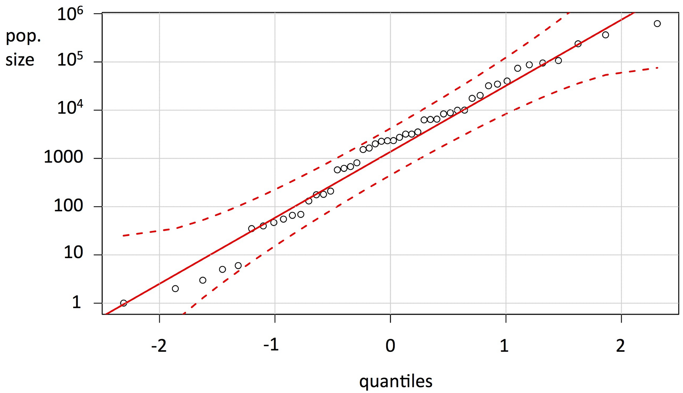
Graph of census populations (number of mature individuals, log scale) of the endemic flora of St Helena (Table 2), as a quantile-quantile (QQ) plot, showing the variation in absolute population sizes of the endemic plants.
Species Half-Lives, Time to Extinction, and the Time Course of Extinction
There is evidence that all species in this analysis are declining. Habitat is progressively being lost and a comparison of fieldwork carried out in the 1980s and a recent survey (2013–4) indicates that there has been a general decline. In some species, this has been dramatic, in others minimal. In only one species (B. lichtensteiniana) is there no obvious evidence of a decline, although some decline is suspected due to plant invasion in native habitats [however, this is partially offset by this being the only endemic plant to have expanded into new anthropogenic habitats, viz., Acacia longifolia (Andrews) Willd. plantations).
Species declines were individually quantified in the form of a time (years) to 50% percent decline (TPD50), or half-life. B. lichtensteiniana, for which there is minimal evidence of decline, is accordingly given a very large TPD50 (10,000) with a high uncertainty (range of 5000–100,000). In contrast, H. saururus has a tiny population and is considered likely to be affected by environmental fluctuations (drought, landslides). It is given a TPD50 of 15 with a range of 5–40 (Table 2).
The half-life can be used to calculate an estimate of the time to critical population thresholds, such as < 1 individual (in our model rounded down to 0, i.e., extinction; see section “Materials and Methods”), 10 individuals (arbitrarily chosen as a critically low population size) and 50 (commonly taken as a threshold of genetic viability, but see Frankham et al., 2014). The build-up of extinct species (or species reaching the other thresholds) can then be projected forward. These forward projections are given in Table 3 and Figure 2. On the basis of this, we can estimate the overall extinction rate for the next 200 years as 625 E/MSY (individual species have different lifespans and different population processes, and move toward extinction at different rates, but this is the overall figure). This is remarkably similar to the directly measured historical extinction rate of 581 E/MSY despite being independently estimated using different data. However, the data do suggest that numerous extinctions are coming up imminently, and over the next 50 years some one to five plant extinctions in St Helena are plausible (central estimate four). In addition, a further seven to nine species are estimated to drop below a population size of 50 (often used as a crude threshold for genetic viability). Figure 3 shows the full extinction time course by joining together the three segments: 1502–1771 (estimated), 1771–2017 (empirical), and 2017–2517 (projected).
TABLE 3
| Time in future (years) | Number of extinctions (n=≤1) | Number of species with < 10 individuals | Number of species with < 50 individuals |
| 0 | 0 | 5 | 8 |
| 50 | (1-)4(-5) | (1-)6(-8) | (9-)11(-12) |
| 100 | (4-)4(-8) | (4-)7(-11) | (11-)12(-13) |
| 150 | (4-)5(-9) | (4-)10(-14) | (11-)13(-16) |
| 200 | (4-)6(-10) | (4-)11(-15) | (11-)13(-17) |
| 500 | (8-)14(-16) | (8-)15(-20) | (14-)18(-24) |
| 1000 | (11-)16(-23) | (11-)19(-27) | (17-)19(-31) |
Projection of extinctions in the wild, and other thresholds, forward in time based upon estimated rates of decline of natural populations.
The central estimate is given together with low and high figures to indicate uncertainty. The number of species with NMI < 10 (i.e., 1–9) is given as these species are considered imminently extinction prone. The < 50 (1–49) column is given as this population size is often used as a rough threshold of population genetic viability for out-breeding species.
FIGURE 2
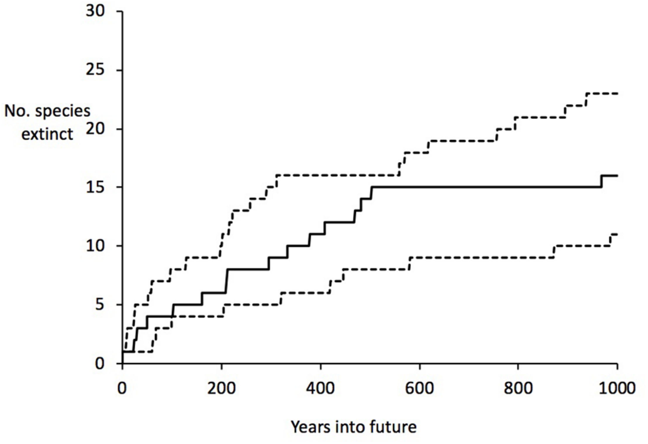
Projected extinctions over time (next 1000 years), based on current threat levels. Upper and lower estimates are given as well as the central estimate (middle).
FIGURE 3
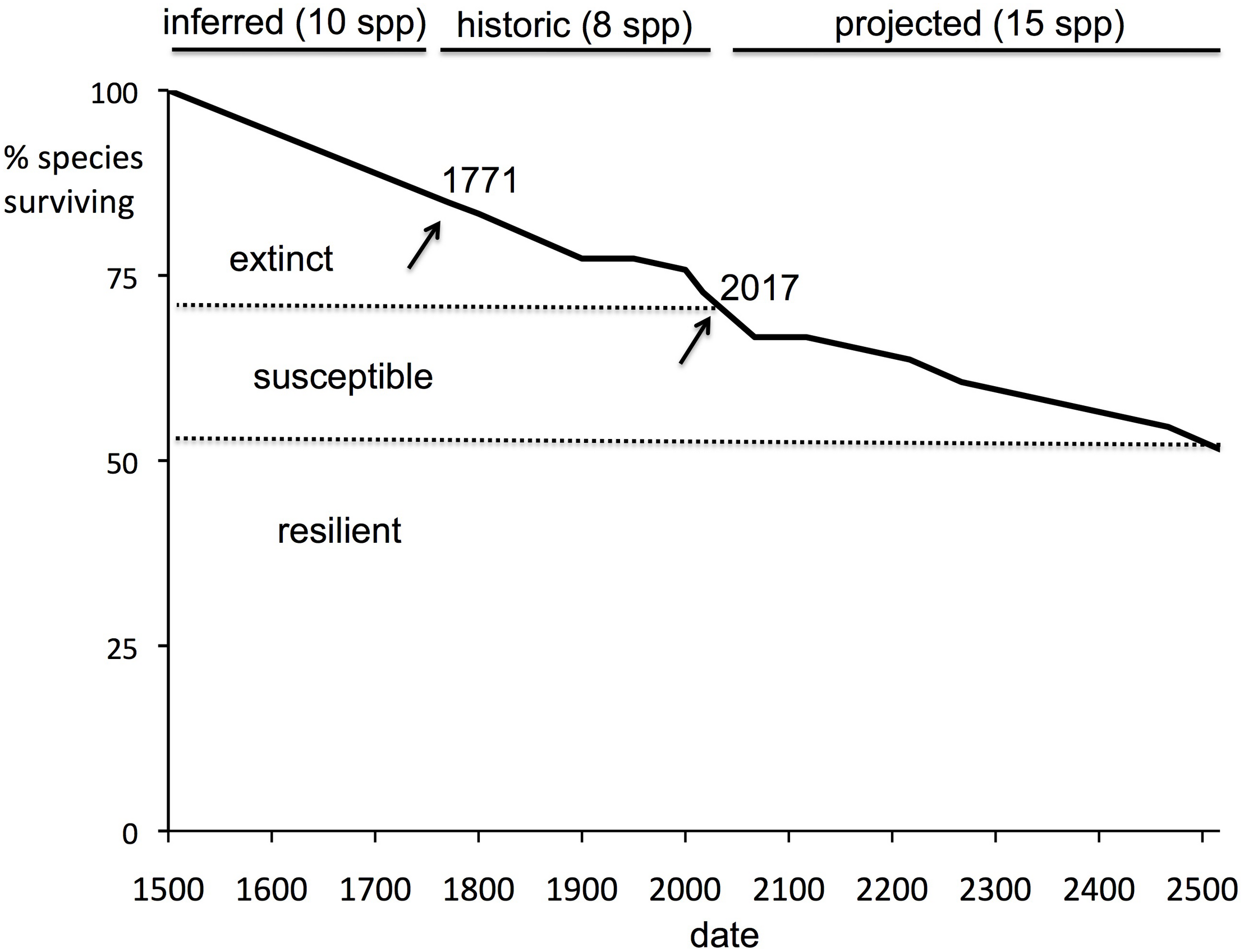
Extinction time course, 1502–2517 as percentage of total flora. A summary of the extinction dynamics of St Helena. “Historic” is actual data; “inferred” is an extrapolation back to 1502 of the historic extinction rate; and “projected” is calculated from a model of current species declines. Despite native ecosystems being reduced to some 3.5% of original levels, less than 30% of the endemic flora is extinct.
Time Course of Habitat Destruction and the Species–Area Curve
St Helena is a small island with an area of 121.7 km2. We estimate that the area occupied by endemic plants has dropped from c. 100% (in 1502) to c. 3.5% today. Superficially, it may seem that habitat destruction has stopped as all remaining areas with native plants are under protection. However, the actual area available to native plants within a protected area is a function of habitat quality. The continuous onslaught of invasive plants does mean that the habitat quality of many of the remaining native plant areas is declining, and so therefore is the effective HA. When the estimated rate of habitat destruction over time is combined with species loss over the same time period, the relationship between HA remaining and species surviving can be determined, i.e., an extinction species–area curve (Figure 4). Our curve follows well the classic S = cAz model (where S is the number of species remaining, A is the HA remaining, and c and z are constants) but with a rather low value for the exponent z (0.1).
FIGURE 4
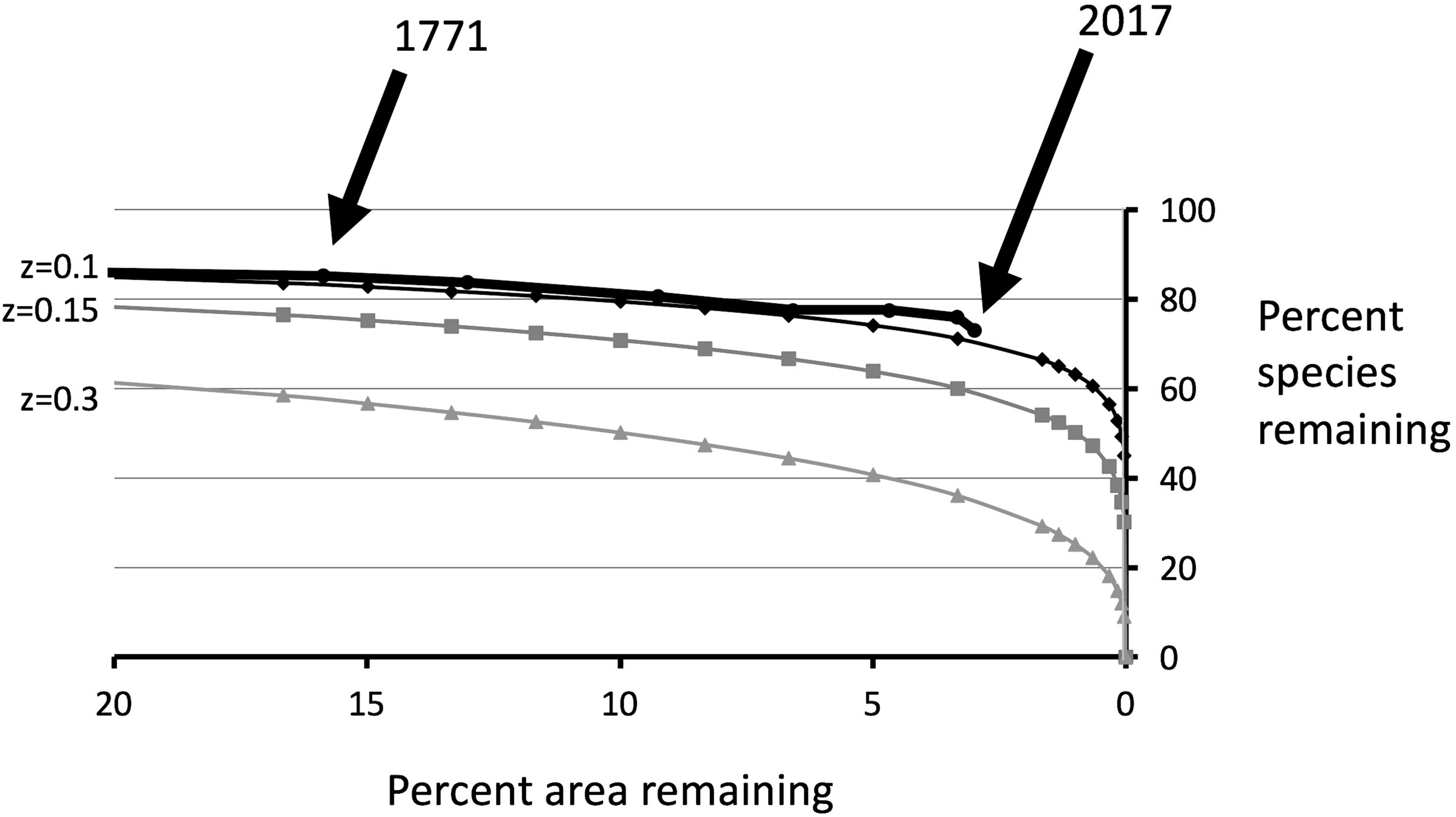
Thick line: estimated species–area curve for extinction due to habitat destruction (actual). Other lines give theoretical curves based on the species–area curve S = cAz, with different values for z. The historical species–area curve matches fairly closely the theoretical curve based on z = 0.1.
Discussion
The Extinction Rate and Extinction-Area Curve for St Helena Is Shallow and Approximately Linear
The area of St Helena now occupied by endemic plants is reduced to around 3.5% of the land surface. As shown in Figure 4, the destruction of natural vegetation over the remaining 96.5% has caused appreciable historical extinction. A simple SAR curve prediction (e.g., S = cAz) with a commonly found value of the exponent (z) of 0.2, would suggest that a larger number of species should have become extinct than is actually the case (Figure 4). However, the observed data fits well with a value of z of 0.1, which is low but still biologically plausible.
We suggest that this low value of z is due to the relaxation time (i.e., a lag time for extinction which makes species survival seem more resistant to habitat destruction than is actually the case). Relaxation time (i.e., time taken to reach new equilibrium) may be particularly long for woody plants (Cronk, 2016). It should be noted that other models have been put forward for the relation between area and extinction (e.g., He and Hubbell, 2011, 2013) which may be appropriate in specific circumstances (Keil et al., 2015). However, the simple SAR is statistically well founded (Pereira et al., 2012; Axelsen et al., 2013) and in this St Helena case, the SAR remains a remarkably good approximation of actual extinction loss.
Extinction Debt
Extinction has a lag phase caused by individual plant longevity and the time needed for stochastic processes to play out as the system attains a new post-disturbance equilibrium. SAR-based estimates of extinction with a relatively steep extinction curve (z = 0.15–0.3) may be seen as giving the equilibrium measure rather than the instantaneous measure: they do not take into account the delayed extinction (relaxation time) as a new equilibrium is reached. This delay of extinction can be characterized as “extinction debt” (Triantis et al., 2010; Halley et al., 2016) alternatively called “biodiversity surplus,” and is the difference between functional extinction and census extinction. A large amount of unpaid extinction debt may thus explain the rather shallow extinction curve (z = c. 0.1) in the observed extinction SAR. If we accept this, then the difference in species at a given area between the number observed (z = 0.1) and that estimated from typical z values of between 0.15 and 0.3 (Price et al., 2018) will give some idea of the magnitude of extinction debt. Following this logic, the extinction debt in 1771 was between four and 14 species and the present extinction debt (2017) is between seven and 20 species. Given that the extinction debt of 1771 was partially resolved by eight extinctions during this time period, up to an additional 14 species must have moved into extinction debt between 1771 and 2017 to maintain the levels of inferred extinction debt. Given the extreme rarity of many endemics and the continuous habitat degradation in St Helena, these numbers are plausible.
An alternative way of exploring extinction debt is through the half-time of debt resolution. An important recent paper (Halley et al., 2016) has provided tools to quantify the decay of extinction debt over time (generations), i.e., the expected time for half the extinction debt to be paid off (t50). Using the equation provided (Halley et al., 2016; Eq. 7, p. 4) together with the constants they estimate for plants (α = 0.48; k = 0.92), the total number of individuals remaining (1.8M; Table 2) and an average generation time of 3 years, we arrive at a t50 of 384 years. This very long relaxation time means that potentially only a portion of the plants that became functionally extinct in the 16th century with the depredations of goats are likely to have already manifested as census extinctions.
Dark Extinction
There may be a much larger amount of unrecorded extinction (pre-1771) than we predict. We call this “dark extinction,” anthropogenic species extinction that is cryptic in that it occurs before a species has been collected and named. This extinction can be inferred but is unlikely ever to be confirmed. However, if there is more dark extinction on St Helena than the 10 species we estimate, then we would expect to see the tail-end of this extinction wave in the records of the first botanists to examine St Helena (i.e., plants almost extinct at the time W. J. Burchell made the first extensive botanical collections from 1805). Actually, there are only two: T. melanoxylon that became extinct just before Burchell arrived and Heliotropium pannifolium, of which Burchell saw only the last individual of the species. The other plants found by Burchell survived much longer, in most cases into the 20th century. There is thus no evidence for an early extinction wave.
Implications for Conservation
The methods used here, using present day decline rates based on present day threats (mainly current levels of plant invasion), predict significant future plant extinction on St Helena (Figure 2).
However, it is quite possible that future threat levels may be much higher, so our predictions will turn out to be underestimates for the following reasons. Climate change may increase the frequency and severity of droughts and other extreme weather events. The threat from invasive plants and pests (mainly insects and microbial pathogens) has increased over time and may get worse. The lag phase and the attendant extinction debt may mean that the current number of realized extinctions is relatively low but likely to increase as the extinction debt is “paid off.” All the remaining safe areas for endemics are small and now exist within a sea of invasive plants. It is therefore quite plausible that over time safe sites will be increasingly eroded by invasion. If the tide of invasion cannot be turned, all the endemic plants of St Helena may be lost and that extinction rate may accelerate as areas get smaller and smaller.
With very small remaining areas, it may not be enough to preserve them in order to conserve all the remaining species from extinction, as genetic and ecological allee effects (Willi et al., 2005; Berec et al., 2007; Luque et al., 2016) may still continue species decline.
General Implications
Because St Helena suffered devastating ecological change by the introduction of the goat shortly after the discovery of the island in 1502, there has been time for some initial extinction debt to have been resolved and a relatively large number of extinctions to occur. It is thus gives an early indication of extinction to come in more recently disturbed ecosystems. Taking the global terrestrial system as a whole, 40% of land area (Steffen et al., 2015) has been “domesticated” (i.e., converted to crop agriculture, grazing land, urban areas, etc.). Although common species, and weeds, may persist and even thrive in these newly converted “agroscapes,” these areas are essentially lost to the majority of biodiversity. Yet this 40% habitat loss has been accompanied by a mere 0.17% loss of seed plant species (Humphreys et al., 2019): 571 seed plant extinctions worldwide out of 334,322 described species. This habitat loss has mainly occurred only over the last 100 years (Steffen et al., 2015) and it is likely that there is considerable extinction debt. Given that extinction debt on St Helena appears to have taken hundreds of years to resolve, it may be the small number of globally extinct plants represents the tip of a large advancing front of extinction.
Conclusion
We have calculated the extinction rate since 1771 as 581 E/MSY. We have also used census data and population decline estimates to project likely extinction forward in time. The projected overall extinction rate for the next 200 years is similar although somewhat higher at 625 E/MSY. However, our data predict an extinction crunch in the next 50 years with four species out of the remaining 48 likely to become extinct during this period. During a period when the native plant areas dropped to 3.5% of the original, the extinction rate appears to have remained approximately shallowly linear with under 30% of the endemic flora becoming extinct, consistent with a species–area curve (S = cAz) with an exponent (z) of c. 0.1.
Taken all together the prognosis leaves no room for complacency. Significant conservation efforts by the St Helena Government and non-Governmental organizations date back at least to the 1970s (Cronk, 1981) but did not prevent the extinction in the wild of Lachanodes arborea (extinct 2012) and the total extinction (in the wild and in cultivation) of the monotypic endemic genus Nesiota (represented by the single endemic species Nesiota elliptica). An aggressive program considering both habitat restoration and the conservation of genetic diversity may be necessary to maintain some species. If that is impossible under current circumstances, then cultivation or seed-banking, until such time that ecosystems can be restored, may be the only option.
Statements
Data availability statement
The data analyzed for this study and associated metadata have been deposited in the Dryad repository (https://datadryad.org/stash/) at https://doi.org/10.5061/dryad.sbcc2fr32.
Author contributions
PL conceived the study and conducted the fieldwork. QC and PL were responsible for conceptual development, analyzed the data, wrote the manuscript, and approved it for publication.
Funding
Funding was provided by the Department for Environment, Food and Rural Affairs (DEFRA) of the UK Government, under the Darwin Plus: Overseas Territories Environment and Climate Fund (Project No. DPLUS008 to PL). We also thank the Natural Sciences and Engineering Research Council of Canada (NSERC) Discovery Grants Program for funding (Grant No. RGPIN-2014-05820 to QC).
Acknowledgments
We thank Shayla Ellick for her contribution to the survey work. We also acknowledge the many people, past and present, who have contributed to conservation efforts of the St Helena flora and who have given hope for the continued survival of the endemic flora. We also acknowledge Dr. Fangliang He (University of Alberta) for helpful general discussions concerning extinction. Finally, we also thank the three referees whose comments greatly improved the manuscript.
Conflict of interest
The authors declare that the research was conducted in the absence of any commercial or financial relationships that could be construed as a potential conflict of interest.
References
1
Axelsen J. B. Roll U. Stone L. Solow A. (2013). Species–area relationships always overestimate extinction rates from habitat loss: comment.Ecology94761–763. 10.1890/12-0047.1
2
Berec L. Angulo E. Courchamp F. (2007). Multiple Allee effects and population management.Trends Ecol. Evol.22185–191. 10.1016/j.tree.2006.12.002
3
Cardoso P. Erwin T. L. Borges P. A. New T. R. (2011). The seven impediments in invertebrate conservation and how to overcome them.Biol. Conserv.1442647–2655. 10.1016/j.biocon.2011.07.024
4
Ceballos G. Ehrlich P. R. Barnosky A. D. García A. Pringle R. M. Palmer T. M. (2015). Accelerated modern human–induced species losses: entering the sixth mass extinction.Sci. Adv.1:e1400253.
5
Ceballos G. Ehrlich P. R. Dirzo R. (2017). Biological annihilation via the ongoing sixth mass extinction signaled by vertebrate population losses and declines.Proc. Natl. Acad. Sci. U.S.A.114E6089–E6096. 10.1073/pnas.1704949114
6
Costello M. J. May R. M. Stork N. E. (2013). Can we name Earth’s species before they go extinct?Science339413–416. 10.1126/science.1230318
7
Cronk Q. C. B. (1981). Senecio redivivus [Lachanodes arborea] and its successful conservation in St Helena.Environ. Conserv.8125–126. 10.1017/S0376892900027156
8
Cronk Q. C. B. (1983). The decline of the Redwood Trochetiopsis erythroxylon on St Helena.Biol. Conserv.26163–174. 10.1016/0006-3207(83)90064-2
9
Cronk Q. C. B. (1986a). The decline of the St Helena ebony Trochetiopsis melanoxylon [T. ebenus].Biol. Conserv.35159–172. 10.1016/0006-3207(86)90048
10
Cronk Q. C. B. (1986b). The decline of the St Helena gumwood Commidendrum robustum.Biol. Conserv.35173–186. 10.1016/0006-3207(86)90049
11
Cronk Q. C. B. (1988). W.J. Burchell and the botany of St Helena.Arch. Nat. Hist.1545–60. 10.3366/anh.1988.15.1.45
12
Cronk Q. C. B. (1989). The past and present vegetation of St Helena.J. Biogeogr.1647–64. 10.2307/2845310
13
Cronk Q. C. B. (1995). A new species and hybrid in the St Helena endemic genus Trochetiopsis.Edinb. J. Bot.52205–213. 10.1017/S0960428600000962
14
Cronk Q. C. B. (2000). The Endemic Flora of St Helena.Oswestry: A. Nelson.
15
Cronk Q. C. B. (2016). Plant extinctions take time.Science353446–447. 10.1126/science.aag1794
16
De Vos J. M. Joppa L. N. Gittleman J. L. Stephens P. R. Pimm S. L. (2015). Estimating the normal background rate of species extinction.Conserv. Biol.29452–462. 10.1111/cobi.12380
17
Di Fonzo M. Collen B. Mace G. M. (2013). A new method for identifying rapid decline dynamics in wild vertebrate populations.Ecol. Evol.32378–2391. 10.1002/ece3.596
18
Diamond J. M. (1972). Biogeographic kinetics: estimation of relaxation times for avifauna of southwest Pacific Islands.Proc. Natl. Acad. Sci. U.S.A.693199–3203. 10.1073/pnas.69.11.3199
19
Díaz S. Settele J. Brondízio E. Ngo H. T. Guèze M. Agard J. et al (2019). Summary for Policymakers of the Global Assessment Report on Biodiversity and Ecosystem Services of the Intergovernmental Science-Policy Platform on Biodiversity and Ecosystem Services.Bonn: IPBES.
20
Fowler S. V. (2004). Biological control of an exotic scale, Orthezia insignis Browne (Homoptera: Ortheziidae), saves the endemic gumwood tree, Commidendrum robustum (Roxb.) DC. (Asteraceae) on the island of St. Helena.Biol. Control29367–374. 10.1016/j.biocontrol.2003.06.002
21
Franken R. J. Hik D. S. (2004). Influence of habitat quality, patch size and connectivity on colonization and extinction dynamics of collared pikas Ochotona collaris.J. Anim. Ecol.73889–896. 10.1017/S00306053120003121-9
22
Frankham R. Bradshaw C. J. Brook B. W. (2014). Genetics in conservation management: revised recommendations for the 50/500 rules, Red List criteria and population viability analyses.Biol. Conserv.17056–63. 10.1016/j.biocon.2013.12.036
23
Gray A. (2019). The ecology of plant extinction: rates, traits and island comparisons.Oryx53424–428. 10.1017/S0030605318000315
24
Gray A. Wilkins V. Pryce D. Fowler L. Key R. S. Mendel H. et al (2019). The status of the invertebrate fauna on the South Atlantic island of St Helena: problems, analysis, and recommendations.Biodiv. Conserv.28275–296. 10.1007/s10531-018-1653-4
25
Halley J. M. Monokrousos N. Mazaris A. D. Newmark W. D. Vokou D. (2016). Dynamics of extinction debt across five taxonomic groups.Nat. Comm.7:12283. 10.1038/ncomms12283
26
He F. Hubbell S. P. (2011). Species-area relationships always overestimate extinction rates from habitat loss.Nature473368–371. 10.1038/nature09985
27
He F. Hubbell S. P. (2013). Estimating extinction from species–area relationships: why the numbers do not add up.Ecology941905–1912. 10.1890/12-1795.1
28
Humphreys A. M. Govaerts R. Ficinski S. Z. Lughadha E. N. Vorontsova M. S. (2019). Global dataset shows geography and life form predict modern plant extinction and rediscovery.Nat. Ecol. Evol.31043–1047. 10.1038/s41559-019-0906-2
29
Janzen D. H. (2001). “Latent extinction - the living dead,” in Encyclopedia of Biodiversity, ed.LevinS. A., (Cambridge, MA: Academic Press), 590–598. 10.1016/b978-0-12-384719-5.00085-x
30
Keil P. Storch D. Jetz W. (2015). On the decline of biodiversity due to area loss.Nat. Comm.6:8837. 10.1038/ncomms9837
31
Lambdon P. (2012). Flowering Plants & Ferns of St Helena.Newbury: Pisces publications for St Helena Nature Conservation Group.
32
Lambdon P. Ellick S. (2014). A Rare Plant Census of St Helena. Darwin Plus: Overseas Territories Environment and Climate Fund Final Report (DPLUS008). Available at: https://www.darwininitiative.org.uk/documents/DPLUS008/23470/DPLUS008%20FR%20-%20Edited.pdf(accessed February 1, 2020).
33
Lande R. (1993). Risks of population extinction from demographic and environmental stochasticity and random catastrophes.Am. Nat.142911–927. 10.1086/285580
34
Lande R. Orzack S. H. (1988). Extinction dynamics of age-structured populations in a fluctuating environment.Proc. Natl. Acad. Sci. U.S.A.857418–7421. 10.1073/pnas.85.19.7418
35
Liow L. H. Fortelius M. Bingham E. Lintulaakso K. Mannila H. Flynn L. et al (2008). Higher origination and extinction rates in larger mammals.Proc. Natl. Acad. Sci. U.S.A.1056097–6102. 10.1073/pnas.0709763105
36
Luque G. M. Vayssade C. Facon B. Guillemaud T. Courchamp F. Fauvergue X. (2016). The genetic Allee effect: a unified framework for the genetics and demography of small populations.Ecosphere7:e01413. 10.1002/ecs2.1413
37
Malanson G. P. (2008). Extinction debt: origins, developments, and applications of a biogeographical trope.Prog. Phys. Geogr.32277–291. 10.1177/0309133308096028
38
McGuinness K. A. (1984). Species–area curves.Biol. Rev.59423–440. 10.1111/j.1469-185X.1984.tb00711.x
39
Melliss J. C. (1875). St Helena.London: Reeve.
40
Otto R. Garzón-Machado V. del Arco M. Fernández-Lugo S. de Nascimento L. Oromí P. et al (2017). Unpaid extinction debts for endemic plants and invertebrates as a legacy of habitat loss on oceanic islands.Divers. Distrib.231031–1041. 10.1111/ddi.12590
41
Percy D. M. Cronk Q. C. B. (1997). Conservation in relation to mating system in Nesohedyotis arborea (Rubiaceae), a rare endemic tree from St Helena.Biol. Conserv.80135–145. 10.1016/S0006-3207(96)00130-9
42
Pereira H. M. Borda-de-Água L. Martins I. S. (2012). Geometry and scale in species–area relationships.Nature482:E3. 10.1038/nature10857
43
Pimm S. L. Russell G. J. Gittleman J. L. Brooks T. M. (1995). The future of biodiversity.Science269:347. 10.1126/science.269.5222.347
44
Price J. P. Otto R. Menezes de Sequeira M. Kueffer C. Schaefer H. Caujapé-Castells J. et al (2018). Colonization and diversification shape species–area relationships in three Macaronesian archipelagos.J. Biogeogr.452027–2039. 10.1111/jbi.13396
45
Purvis A. (2008). Phylogenetic approaches to the study of extinction.Annu. Ann. Rev. Rev. Ecol. Evol. Syst.39301–319. 10.1146/annurev-ecolsys-063008-10201
46
Snäll T. Ehrlén J. Rydin H. (2005). Colonization–extinction dynamics of an epiphyte metapopulation in a dynamic landscape.Ecology86106–115. 10.1890/04-0531
47
Stanton J. C. Semmens B. X. McKann P. C. Will T. Thogmartin W. E. (2016). Flexible risk metrics for identifying and monitoring conservation-priority species.Ecol. Indic.61683–692. 10.1016/j.ecolind.2015.10.020
48
Steffen W. Broadgate W. Deutsch L. Gaffney O. Ludwig C. (2015). The trajectory of the Anthropocene: the great acceleration.Anthropocene Rev.281–98. 10.1177/2053019614564785
49
Tilman D. May R. M. Lehman C. L. Nowak M. A. (1994). Habitat destruction and the extinction debt.Nature37165–66. 10.1038/371065a0
50
Tollefson J. (2019). One million species face extinction.Nature569:171.
51
Triantis K. A. Borges P. A. Ladle R. J. Hortal J. Cardoso P. Gaspar C. et al (2010). Extinction debt on oceanic islands.Ecography33285–294. 10.1111/j.16000-0587.2010.06203.x
52
Willi Y. Van Buskirk J. Fischer M. (2005). A threefold genetic Allee effect.Genetics1692255–2265. 10.1534/genetics.104.034553
Summary
Keywords
plant extinction, extinction rate, oceanic island, island extinction, St Helena, dark extinction, extinction debt, species–area curve
Citation
Lambdon P and Cronk Q (2020) Extinction Dynamics Under Extreme Conservation Threat: The Flora of St Helena. Front. Ecol. Evol. 8:41. doi: 10.3389/fevo.2020.00041
Received
07 September 2019
Accepted
10 February 2020
Published
26 February 2020
Volume
8 - 2020
Edited by
David Jack Coates, Department of Biodiversity, Conservation and Attractions (DBCA), Australia
Reviewed by
John Maxwell Halley, University of Ioannina, Greece; Aelys Muriel Humphreys, Stockholm University, Sweden; Rui Bento Elias, University of the Azores, Portugal
Updates
Copyright
© 2020 Lambdon and Cronk.
This is an open-access article distributed under the terms of the Creative Commons Attribution License (CC BY). The use, distribution or reproduction in other forums is permitted, provided the original author(s) and the copyright owner(s) are credited and that the original publication in this journal is cited, in accordance with accepted academic practice. No use, distribution or reproduction is permitted which does not comply with these terms.
*Correspondence: Quentin Cronk, quentin.cronk@ubc.ca
This article was submitted to Conservation, a section of the journal Frontiers in Ecology and Evolution
Disclaimer
All claims expressed in this article are solely those of the authors and do not necessarily represent those of their affiliated organizations, or those of the publisher, the editors and the reviewers. Any product that may be evaluated in this article or claim that may be made by its manufacturer is not guaranteed or endorsed by the publisher.