Using Model Analysis to Unveil Hidden Patterns in Tropical Forest Structures

When ordinating plots of tropical rain forests using stand-level structural attributes such as biomass, basal area and the number of trees in different size classes, two patterns often emerge: a gradient from poorly to highly stocked plots and high positive correlations between biomass, basal area and the number of large trees. These patterns are inherited from the demographics (growth, mortality and recruitment) and size allometry of trees and tend to obscure other patterns, such as site differences among plots, that would be more informative for inferring ecological processes. Using data from 133 rain forest plots at nine sites for which site differences are known, we aimed to filter out these patterns in forest structural attributes to unveil a hidden pattern. Using a null model framework, we generated the anticipated pattern inherited from individual allometric patterns. We then evaluated deviations between the data (observations) and predictions of the null model. Ordination of the deviations revealed site differences that were not evident in the ordination of observations. These sites differences could be related to different histories of large-scale forest disturbance. By filtering out patterns inherited from individuals, our model analysis provides more information on ecological processes.

1. Introduction

Among trees in a forest stand, tall trees are expected to have large diameters (because of mechanical and physiological processes operating at intra-tree level). Moreover, tree sizes in a stand are expected to be distributed following a general distribution that reflects population demographical processes (i.e., growth, mortality and recruitment). Therefore, a forest stand with a tall canopy is also expected to have a large basal area and, when considering a collection of forest stands at different developmental stages, stand canopy height and stand basal area are positively correlated. Such a correlation is an example of a pattern, i.e., any structure in observations that is significantly different from a random process realization (Wiegand et al., 2003; Grimm and Railsback, 2012). Patterns are key in ecology to understand and infer underlying ecological processes. We define an obvious pattern as a pattern that is inherited from patterns in the constituent elements that compose the object under study. In the above example, the correlation between canopy height and basal area of a forest stand (= the object under study) is an obvious pattern because it is automatically inherited from the size allometry and demographics of trees (= the constituent elements).

The canopy height of a forest stand is, however, also determined by other factors, such as soil. When plotting canopy height vs. basal area for stands at different developmental stages and soil conditions, the observed correlation will mix the soil effects with the obvious positive correlation between canopy height and basal area inherited from trees. The positive correlation between height and basal area may be dominant to the point that the soil effect is not visible at the first order. Hence, obvious patterns can hide relevant patterns useful in inferring underlying ecological processes: an informative pattern may be hidden by a dominant uninformative pattern. The challenge, then, is to filter out the dominant pattern to reveal the hidden pattern.

Although this paper is method-oriented, we shall for clarity and illustration sake focus on tropical rain forests, where the structure is defined as the set of all stand attributes that depend on tree sizes (such as tree density, basal area, aboveground biomass, mean diameter, but excluding any attribute depending on species composition) (Rollet, 1974). Using a multivariate ordination of forest plots based on their structural attributes (Legendre and Legendre, 1998, chapter 9), we will investigate correlations between these structural attributes and the gradient among forest plots detected by the ordination. Considering biomass, basal area, and the number of small, medium, and large trees, a general pattern in tropical rain forests is sketched in Figure 1. The high positive correlation between biomass, basal area and the number of large trees has been widely reported in the literature across the tropics (Lewis et al., 2013; Bastin et al., 2018). Correlations between other structural attributes can be seen, for instance, in French Guiana (Baraloto et al., 2011), or in central Africa (Palla et al., 2011), even though Baraloto et al. jointly analyzed structural variables and environmental variables. The persistence of the correlations sketched in Figure 1 despite the presence of other, non-structural variables indicates that this pattern is dominant. Along with this pattern, a second pattern emerging from the ordination of forest plots is a gradient from poorly (low biomass, basal area and stem density) to highly (high biomass, basal area and stem density) stocked plots.

FIGURE 1

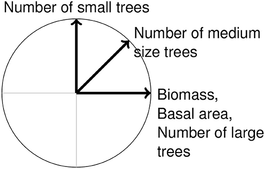
Figure 1. Schematic view of the expected correlation circle between biomass, basal area, and the number of small, medium size, and large trees when ordinating tropical rain forest plots.

Our hypothesis is that these two patterns (gradient from poorly to highly stocked forest plots and correlations sketched in Figure 1) are dominant and obvious patterns that hide more informative patterns. To investigate this hypothesis, we used data from 133 forest plots located at nine tropical sites for which site differences are known.

To filter out the dominant pattern and unveil hidden ones, we use an approach similar to null model analysis (Gotelli and Graves, 1996; Dormann et al., 2017). Gotelli and Graves (1996) defined a null model as “a pattern generating model that is based on randomization of ecological data or random sampling from a known or imagined distribution.” Referring to Gotelli and Ulrich's (2012) terminology (see their Figure 1), this pattern-oriented model (sensu Wiegand et al., 2003) lies somewhere between a statistical test of a null hypothesis using a predefined theoretical distribution and a “mechanistic model” that is process-oriented and does not involve any randomization of data. Hence, “null model analysis specifies a statistical distribution or randomization of the observed data, designed to mimic the outcome of the random process model without specifying or estimating all of its parameters” (Gotelli and Ulrich's, 2012). We develop a null model by combining a parametric component (= a “mechanistic” component in Gotelli and Ulrich's terminology) with a randomization component that consisted of randomizing the deviations of observations to the predictions of the parametric component. The parametric component, which is fitted to the data, assumes an exponential distribution of individual tree diameters to predict stand-level structural attributes. For this model analysis to remove the dominant pattern and reveal hidden patterns, the parametric component of the null model must generate the dominant pattern. We show that after removing the obvious pattern, the correlation between the deviations of structural variables and the ordination of plots based on these deviations provides ecological insights that did not emerge with the classical ordination approach based on observations.

2. Materials and Methods

2.1. Model Analysis

The model in our analysis consists of a parametric component and a randomization component. The parametric component is based on processes operating at the tree level (growth, mortality, recruitment, allometry…), but does not include any processes that may generate site differences. The plot-level pattern that it generates is thus obvious in the sense that it is automatically inherited from tree attributes. The randomization component cumulates the parametric tree-level predictions while ensuring that the resulting plot-level predictions are consistent with observations. The randomization process removes any pattern in the deviations between observations and the predictions of the parametric component.

2.1.1. Parametric Component of the Model

Given n forest plots and a set of p variables that characterize the forest structure (tree density, basal area, aboveground biomass, mean diameter, or the number of trees in different diameter classes, etc.), the parametric component of the model generates the structural variables of each plot based on mechanisms operating at the tree level. Like Gotelli and Graves (1996), we prefer simple and parsimonious models that can account for the dominant pattern at the plot level. We assume that all trees within each plot had constant growth, mortality, and recruitment rates. Moreover, we assume that all trees in all plots have a constant wood density ρ of 0.6 g cm⁻³ and that their biomass-diameter allometry is the same as given by Chave et al.'s (2005) equation for moist forests: f(x, ρ) = ρexp[−1.499+2.148ln x+0.207(ln x)²−0.0281(ln x)³], with x the tree diameter in cm and f(x, ρ) its biomass in kg. These simple assumptions do not include any mechanism related to site differences (e.g., growth dependence on environmental conditions) and ensure that any plot-level pattern generated by the parametric component is inherited from the tree-level patterns contained in these assumptions. Constant demographic rates (growth, mortality, recruitment) at the tree level imply that the stationary diameter distribution at the plot level is an exponential distribution with density function Nμexp[−μ(x−x₀)], where x is tree diameter, x₀ is the minimum diameter for inventory (a constant imposed by the sampling design of the forest inventory), μ equals the ratio of the mortality rate to the diameter growth rate, and N equals the ratio of the recruitment rate over the mortality rate (Supplementary Text 1). The diameter distribution sums to N, the density of trees in each plot. This exponential diameter distribution adheres to the reverse-J shaped diameter distribution of undisturbed tropical forests (Rollet, 1974) and ensures that the pattern generated by the parametric component is the observed dominant pattern.

An alternative to the assumption of constant demographic rates is metabolic scaling theory that also generates a reverse-J shaped diameter distribution at the plot level (Muller-Landau et al., 2006). Metabolic scaling theory results in a size distributions following a power law. We also explore this option (as Supplementary Material) to assess the sensitivity of the results to the choice of the parametric component of the model.

Given the diameter distribution, the wood density ρ, and the allometric equation f, all plot-level structural variables considered in this study can be computed as specified in Table 1. The two parameters N and μ of the diameter distribution have to be estimated for each plot. We may equivalently reparameterize the distribution using any two structural variables such that N and μ are identifiable from these two variables. In practice, we used tree density N and basal area G, and fitted the diameter distribution to each plot i by minimizing the distance between the centered and scaled vector of observed structural variables and the centered and scaled vector of predicted structural variables:

$\begin{array}{ll}({\widehat{N}}_i,{Ĝ}_i)=arg{\displaystyle \underset{N,G}{min}}{\displaystyle \sum _{j=1}^p}\frac{{[A_{\text{obs},ij}-A_{\text{mod},j}(N,G)]}^2}{s_j^2}& (1)\end{array}$

where A_{mod, j}(N, G) is the predicted jth structural variable (i.e., one of the structural variables given in Table 1) for a plot with tree density N and basal area G (j = 1, …, p), A_{obs, ij} is the observed jth structural variable (j = 1, …, p) of the ith plot (i = 1, …, n), and $s_j^2$ is the variance of A_{obs, ij} across the n plots.

TABLE 1

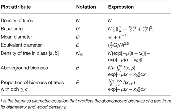
Table 1. Expression of the plot attributes when the diameter distribution at plot level is modeled by an exponential distribution with parameter μ, given by: Nμexp[−μ(x − x₀)], where x is tree diameter and x₀ is the minimum diameter for inventory (a constant imposed by the sampling design of the forest inventory).

2.1.2. Randomization Component of the Model

Let A_obs be the matrix with n rows, p columns and element A_{obs, ij} that assembles the observed structural variables of all plots. The parametric component of the model defines a matrix A_mod with n rows and p columns whose element at the ith row and jth column equals the fitted value $A_{\mathrm{\text{mod}},j}({\widehat{N}}_i,{Ĝ}_i)$. The difference between the observed matrix A_obs and the model matrix A_mod defines a matrix D of deviations:

$\begin{array}{ll}{\text{A}}_{\text{obs}}={\text{A}}_{\text{mod}}+\text{D}& (2)\end{array}$

Under the null hypothesis, all the pattern in the data of the observed matrix A_obs results from the model, so that there is no pattern in the matrix D of deviations. Following Gotelli and Graves (1996), the pattern in the data is measured by a metric M operating on n × p matrices, while the distribution of M(D) under the null hypothesis is defined by a randomization process that reflects the absence of pattern in D according to the metric M (Gotelli et al., 2011). For instance, when interested in the correlation between the jth and kth variables that characterize the forest structure, a relevant metric is Pearson's correlation coefficient:

$\begin{array}{ll}M(A)=\frac{a_j^{\text{T}}{a}_k-(1^{\text{T}}{a}_j)(1^{\text{T}}{a}_k)}{\sqrt{[a_j^{\text{T}}{a}_j-{(1^{\text{T}}{a}_j)}^2][a_k^{\text{T}}{a}_k-{(1^{\text{T}}{a}_k)}^2]}}& (3)\end{array}$

where a_j is the jth column vector of A, 1 is the vector of length n full of ones, and a^T for any vector a denotes the transpose of a. When interested in the structure of A as a whole, a relevant metric is the sum of the eigenvalues of the first c components of the principal component analysis (PCA) of A, with c the number of components selected to represent the data set sufficiently (Abdi and Williams, 2010; Linting et al., 2011). A randomization process in those cases consists in randomly permuting the elements of each column-vector of D, concurrently and independently from each other (Buja and Eyuboglu, 1992; Linting et al., 2011). Let π₁, …, π_p be p independent random permutations of n elements, and let D_null be the random matrix obtained from D as e_null,j = π_j(e_j), where e_j is the jth column of D. This randomization process removes the entire correlational structure of the data, so that matrix D_null does not present any pattern according to the metric M. Let A_null = A_mod+D_null be a random outcome of the null model.

To test if the pattern in A_obs entirely follows from the parametric model or if extra pattern in A_obs is not accounted for, Gotelli and Graves (1996) compared M(A_obs) to the distribution of M(A_null). In agreement with the idea of filtering out the dominant pattern, and following an approach similar to the ordination of residuals made by Couteron et al. (2003) that was equivalent with a PCA with instrumental variables, we rather compared M(D) to the distribution of M(D_null). The two options are identical when M is linear with respect to A, which is generally not the case. The former option is fine to check if the null model can reproduce the observed pattern. The latter option is better to check if there is a remaining hidden pattern once the obvious dominant pattern has been filtered out. The randomization test indicates whether the pattern in deviations is likely, or not, to have arisen by chance, and does not solve issues of dependence of deviations (such as those resulting from inter-plot spatial autocorrelation) that would lead to type I errors if the test was used to test the absence of correlation between deviations (Legendre and Legendre, 1998, p. 17–26).

2.2. Study Sites and Plots

Forest data came from 133 plots distributed across nine sites, totaling 262.56 ha (Table 2). All forests were tropical broadleaf rain forests (Figure 2), all under tropical climate according to the Köppen-Geiger climate classification, with the seasonal precipitation type being equatorial, monsoonal, wet or dry. The altitude of the sites varied from very low elevation close to the littoral (at Paracou and Oyan) to low elevation (maximum 625 m asl). Soils in all sites were ferralitic soils, mostly ferralsols according to the soil classification of the World Reference Base for Soil Resources, but also including acrisols (with clay-enriched subsoil) and plinthosols (with accumulation of Fe). Most of the sites were located on plateaus interrupted by rivers, with a flat to moderate relief, often consisting of a succession of small round-topped hills. A noticeable exception is the Uppangala site that was located on steep mountain slopes.

TABLE 2

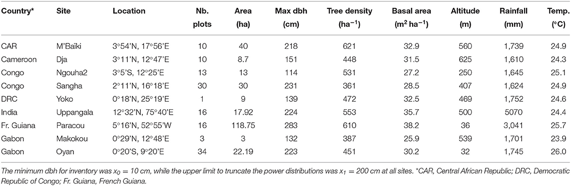
Table 2. Main characteristics of the study sites in terms of sampling effort (number of plots and total inventoried area), structural attributes (maximum dbh, tree density and basal area), and environment (altitude, annual rainfall and average temperature).

FIGURE 2

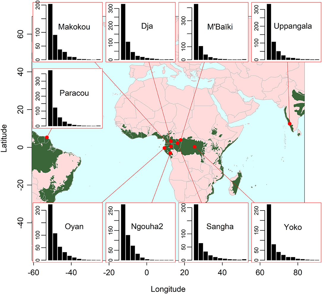
Figure 2. Location of the nine study sites and distribution of the diameter at breast height (dbh) at each site (inset plots). The green area represents the biome of tropical and subtropical moist broadleaf forests as delimited by Dinerstein et al. (2017). In the insets, the eleven bars correspond to the eleven diameter classes 10–20 cm, 20–30 cm, …, 100–110 cm, and ≥ 110 cm, while the y-axis gives the density of trees per hectare.

Sites mainly differed with respect to their species composition and disturbance history. The different floristic assemblages among sites reflected the known large scale patterns in phytogeography (Fayolle et al., 2014b), but also regional bioclimatic patterns (i.e., degree of evergreenness vs. deciduousness of the forest). Two sites, Ngouha2 in Congo and Oyan in Gabon, were exclusively composed of monodominant okoume (Aucoumea klaineana Pierre) forest, with okoume alone representing 56% and 85% of the forest basal area, respectively (Peh et al., 2011). The Dja site in Cameroon also had 40% of its plots located in monodominant limbali [Gilbertiodendron dewevrei (De Wild.) J. Léonard] forest. Monodominance vs. mixed forest could thus be a first factor that differentiates sites.

Most of the plots were initially established in old-growth forest, with no historical evidence of perturbation. However, two-thirds of the plots in the Sangha site in Congo were established in forests that were selectively logged at low intensity (< 2 trees ha⁻¹) in the early eighties. This low intensity logging is still discernible after 35 years in some forest attributes (Poulsen et al., 2013). Three plots at Uppangala were perturbed by a wildfire 30 years ago. Because okoume has a pioneer behavior, monodominant okoume stands at Ngouha2 and Oyan also indicate that large scale disturbances once occurred at those sites (Brunck et al., 1990). Dendrochronology studies conducted at Oyan showed that monodominant patches corresponded to even-aged cohorts of okoume trees with a minimum age of 7–12 years and a maximum age of 50–60 years (Rivière, 1992).

Permanent sample plots were established either as part of an experimental design to study silvicultural techniques for sustainable forest management (M'Baïki, Ngouha2, Oyan, Paracou and Yoko sites), or for ecological research purposes (all other sites). Most of the plots in this latter case were established in protected areas, although some plots were also established in forest logging concessions (Sangha site). In the former case, we used the data measured at the initial time when each plot was established, before any silvicultural treatment. The measurement protocol was similar in all sites, with all trees with a girth at breast height (gbh, measured at 1.3 m above ground) ≥ 30 cm being identified at species or morphospecies level, individually marked, and their gbh measured. Diameter at breast height (dbh) was obtained from gbh assuming a circular cross-section of the trunk. More information on the study sites and plots is given in Supplementary Text 2.

The aboveground biomass of each tree was computed using the allometric Equation (7) by Chave et al. (2014) that depends on tree dbh, wood density and a site-specific bioclimatic stress index. Wood density was determined for each tree species using the global wood density database (Zanne et al., 2009), employing a genus average when no match was found at species level, and a default value of 0.6 g cm⁻³ when no match was found at genus level. Individual tree data were aggregated at the plot level to get the following structural attributes of each plot: density of trees (in total or by diameter class), basal area, mean diameter, equivalent diameter (i.e., the square root of the mean quadratic diameter) and aboveground biomass (in total or by diameter class).

2.3. Analyses

For each of the 133 forest plots, the data were fitted to the model using the optimization defined by Equation (1). Based on the estimated parameters, the predicted structural variables were then computed using the equations in Table 1, and the deviations between observations and predictions were finally computed using Equation (2). Three different sets of structural variables were analyzed using the model analysis.

First, we studied the correlation between biomass and basal area across the 133 permanent sample plots using Peason's correlation coefficient (Equation 3) as the metric and using our randomization process to derive its null distribution. Second, we extended our study of correlation between structural variables under the null model to p = 9 structural variables (density of trees, basal area, mean diameter, equivalent diameter, density of trees with dbh < 30 cm, density of trees with dbh in the range 30–60 cm, density of trees with dbh ≥ 60, aboveground biomass, and proportion of biomass represented by trees with dbh ≥ 60 cm) using the PCA of the centered and scaled variables, and the sum of the eigenvalues of the first two components of the PCA as the metric.

Third, to focus on the diameter distribution only (i.e., disregarding all other tree attributes), we assembled a table of structural variables from the density of trees in 11 dbh classes ranging from 10 to 110 cm with an interval of 10 cm (except the last class that contained all trees with dbh ≥ 110 cm). This 133 × 11 table of densities was first transformed using the chord transform (Legendre and Borcard, 2018), which was again ordinated using PCA. All analyses were conduced with R software (see Supplementary Text 6).

We repeated the analyses with alternative choices for the parametric component of the null model or data selection to assess the sensitivity of the results to specific model or data features. First, the power model was used as an alternative to the exponential model in the model analysis (see Supplementary Text 3 for the definition of its parametric component). Second, to assess the possible influence of young forest plots on the results, analyses were repeated after removing all plots with basal area < 20 m² ha⁻¹. Third, to assess the influence of variation in wood density, we rebuilt the matrix of observations A_obs using pseudo-observations where tree wood densities were replaced by a constant value of 0.6 g cm⁻³ while keeping all other tree data to their observed values, which is equivalent with deleting site differences in average wood density.

3. Results

3.1. Correlation Between Biomass and Basal Area

Pearson's correlation coefficient between the observed biomass and the observed basal area of the plots was 0.80 (Figure 3A). Beyond this dominant pattern of high positive correlation between biomass and basal area, data presented another pattern related to site differences. Sites could be classified into several groups with Oyan and Ngouha2 having relatively low biomass even for high basal areas (red and orange dots in Figure 3A), the other sites having high biomass for high basal area, and Uppangala lying in between. The exponential null model rendered the dominant pattern of high positive correlation between biomass and basal area (correlation coefficient of 0.98; Figure 3B), showing that this high positive correlation was not linked to site differences and is an obvious pattern. Filtering this pattern out, i.e., correlating the deviations of plot biomass and basal area to model predictions, allowed us to more clearly evidence site differences than when directly correlating observations. The correlation between the deviations of biomass and basal area to the predictions equaled −0.49 and was significantly different from zero (p < 0.001).

FIGURE 3

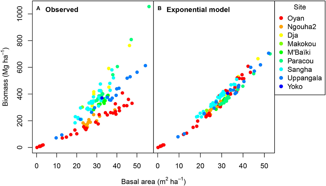
Figure 3. Aboveground biomass vs. basal area for 133 forest stands at nine sites as (A) observed and (B) predicted by the exponential null model. The different colors correspond to the different sites as shown in the legend.

We can check that the correlation in deviations resulted from differences between Oyan and Ngouha2 and the other sites by excluding the data from these two sites. The correlation between observed biomass and basal area then was 0.87, while the correlation between modeled biomass and basal area was 0.96. The correlation between the deviations of biomass and basal area to the predictions was < 0.01 and was not significantly different from zero (p = 0.96). Even if the pattern of correlation in the data was well rendered by the exponential null model, it is worth noting that the null model predicted a smaller slope for the response of biomass to basal area than actually observed (compare Figure 3A where biomass reaches 1,000 Mg ha⁻¹ for the highest basal areas, and Figure 3B where biomass remains below 700 Mg ha⁻¹). These differences are not measurable with a metric like the correlation coefficient.

Replacing the exponential model with the power model (Supplementary Text 3) or removing plots with basal area < 20 m² ha⁻¹ (Supplementary Text 4) had little influence on the results. Imposing the same wood density for all trees changed the correlation pattern between biomass and basal area, with the Oyan and Ngouha2 plots becoming more aligned with the Uppangala plots (Supplementary Text 5). A remaining pattern due to site differences (beyond those associated with wood density) was still significant. The model analysis was more sensitive to the deletion of site differences in wood density (correlation coefficient of deviations to model predictions changing its sign from −0.49 to 0.31) than the direct correlation analysis based on observations (correlation coefficient changing from 0.80 to 0.93).

3.2. Ordination of Plots Based on Structural Variables

The PCA of structural characteristics showed the general pattern of Figure 1, with a strong positive correlation between basal area, biomass and the density of trees with dbh ≥ 60 cm on the first axis of the PCA, and a strong positive correlation between the overall tree density and the density of trees with dbh < 30 cm on the second axis of the PCA (Figure 4A). The sum of the first two eigenvalues was 7.4. The projection of plots on the first two axes of the PCA opposed plots with large basal area or biomass to those with small basal area or biomass (1st axis), and plots with large tree density to those with small density (2nd axis; Figure 4B). This ordination of plots corresponded to the expected general pattern and did not separate forest sites well. The exponential null model rendered well the dominant pattern of observed data (compare Figures 4A,C and Figures 4B,D), with a more structured pattern than observed as shown by the proximity of variable loadings to the border of the circle in Figure 4C. The sum of the first two eigenvalues for the exponential model equaled 8.7.

FIGURE 4

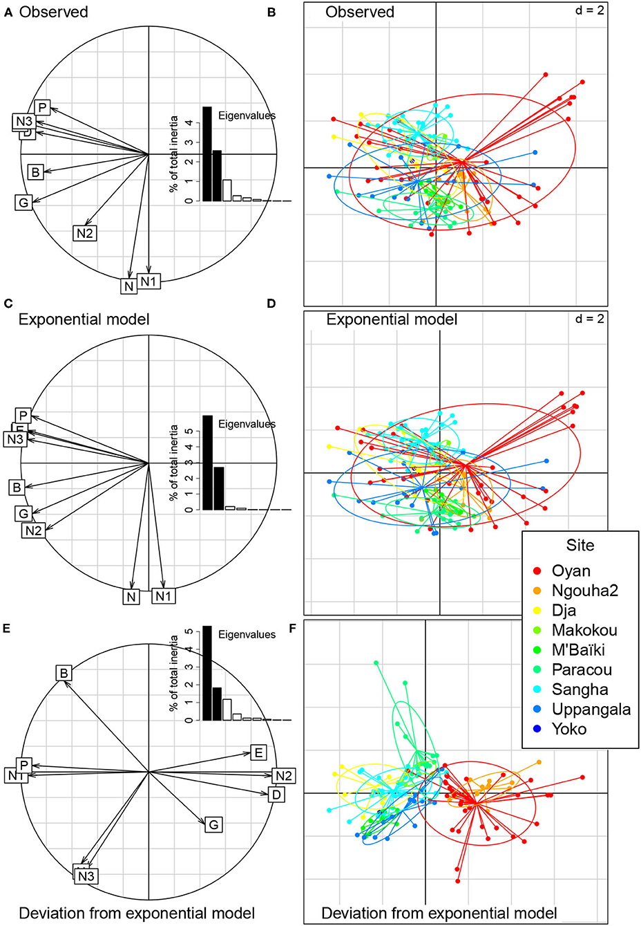
Figure 4. Principal component analysis (PCA) of structural characteristics of 133 forest plots at nine sites. The PCA is performed either on the matrix of observed data (A,B), on the modeled data using the exponential model (C,D), or on the deviations of observations to the predictions of the exponential model (E,F). (A,C,E) Correlation circle between the first two axes of the PCA and structural characteristics (N = density of trees, G = basal area, D = mean diameter, E = equivalent diameter, N₁ = density of trees with dbh < 30 cm, N₂ = density of trees with dbh in the range 30–60 cm, N₃ = density of trees with dbh ≥ 60, B = aboveground biomass, and P = proportion of biomass represented by trees with dbh ≥ 60 cm). The insets show the eigenvalues of the PCA. (B,D,F) Projection of the forest plots on the first two axes of the PCA. Each dot corresponds to a plot with the color indicating the site. Lines and ellipses highlight the dispersion of the plots of each site.

The PCA of the deviations of the structural variables fitted with the exponential model offered a very different view of the forest structure (Figures 4E,F). The matrix of deviations D showed a significant pattern (sum of first two eigenvalues = 7.1, p < 0.001). Two groups of sites were separated along the first axis of the PCA: Oyan and Ngouha2 on the one hand, and the other sites on the other hand (Figure 4F). This first axis was mainly built on a negative correlation between the deviation of the density of trees with dbh in the range 30-60 cm and the deviation of the density of trees with dbh < 30 cm (Figure 4E). Therefore, plots in the Oyan and Ngouha2 sites had more trees in the 30-60 cm dbh class and fewer trees in the dbh class < 30 cm than expected under the null model as compared to the other sites. The model analysis revealed a pattern of site differences that was not perceptible with the PCA of observations.

The power null model performed slightly less well than the exponential model in rendering the dominant pattern of observed data, but results were similar for both models (Supplementary Text 3). Removing plots with basal area < 20 m² ha⁻¹ had little influence on the results, but accentuated the contrast between the PCA of observations and the PCA of deviations to the null model (Supplementary Text 4). Oyan and Ngouha2 sites were more superimposed with other sites in the analysis of observations and more clearly separated from other sites in the analysis of deviations to the null model when plots with basal area < 20 m² ha⁻¹ were excluded than when included. Imposing a constant wood density on all trees had little influence on the results of the PCA (Supplementary Text 5), except for the change of sign of the correlation between the deviation of biomass and the deviation of basal area reported above.

3.3. Ordination of Plots Based on Densities in dbh Classes

The main gradient of the PCA of chord-transformed trees densities in dbh classes was again a gradient of poorly to highly stocked plot (Figure 5A). The sum of the first two eigenvalues was 7.9. Plots with a high score on the first axis of the PCA had a greater density of trees in the smallest dbh class and a smaller density of trees in the intermediate classes, implying a steep dbh distribution. Conversely, plots with a small score on the first axis had a smaller density of trees in the smallest dbh class, implying a flatter dbh distribution. Again site differences were not clearly visible along this dominant gradient with the plots of the Oyan site covering the whole gradient along the first axis (Figure 5B). The second axis of the PCA separated sites to some extent. The exponential null model rendered the dominant gradient along the first axis of the PCA, with an amplification of the opposition between poorly stocked plots with more trees in the smallest dbh classes and highly stocked plots with more trees in the intermediate dbh classes (Figures 5C,D). The sum of the first two eigenvalues for the exponential model equaled 10.9.

FIGURE 5

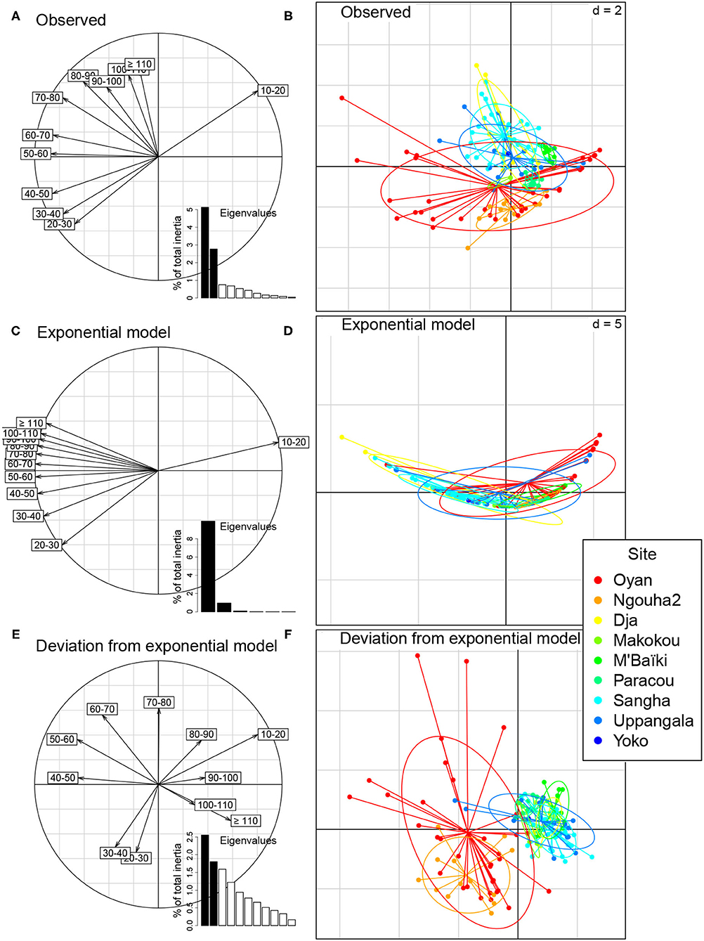
Figure 5. Principal component analysis (PCA) of the chord-transformed abundances of stems per dbh class in 133 forest plots at nine sites. The PCA is performed either on the matrix of observed abundances (A,B), on the modeled abundances using the exponential model (C,D), or on the deviations of observations to the predictions of the exponential model (E,F). (A,C,E) Correlation circle between the first two axes of the PCA and the chord-transformed abundances in the dbh classes (from 10 to 20 cm for the first dbh class to ≥ 110 cm for the 11th dbh class). The insets show the eigenvalues of the PCA. (B,D,F) Projection of the forest plots on the first two axes of the PCA. Each dot corresponds to a plot with the color indicating the site. Lines and ellipses highlight the dispersion of the plots of each site.

The PCA of the deviations from the null model again offered a very different view of the forest structure. There was a significant pattern left in the deviations of observations from the exponential model (sum of the first two eigenvalues = 4.4, p < 0.001). The Oyan and Ngouha2 sites were separated from the other sites along the first axis (Figure 5F). This axis contrasted plots with tree densities in the smallest or greatest dbh classes that strongly deviated from the null model, and those for which the deviation was strongest in intermediate dbh classes (Figure 5E). The analysis again revealed a pattern of site differences that was not perceptible along the main dominant gradient of the PCA of observations.

4. Discussion

4.1. The Gradient of Plots Is a Dominant and Obvious Pattern That Hides Site Differences

The dominant pattern captured by the ordination of forest plots was a gradient from a steep reverse-J distribution to a flatter reverse-J distribution. This signal was strong enough for similar results to be obtained with the PCA of structural variables and the PCA of densities in dbh classes. This dominant pattern is widely reported in tropical forests, whether based on the PCA of structural attributes (Baraloto et al., 2011; Palla et al., 2011) or on the correspondence analysis of the densities of trees in dbh classes (Couteron et al., 2003; Fayolle et al., 2014a). This pattern is so general that the reverse-J dbh distribution has been suggested as a way to assess disturbance (Sellan et al., 2017).

This dominant gradient of plots is rendered by a null model that accounts for tree allometry and constant demographic rates in growth, mortality and recruitment. Therefore, it is inherited from tree patterns and is an obvious gradient. Site differences only had a second-order influence on the gradient of plots. They were more clearly visible in the analysis of the deviations to the null model than in the original observations where they were hidden by the dominant obvious pattern.

The dataset used in this study originated from well-documented sites, allowing us to confirm the ecological insights on site differences revealed by the null model analysis. The Ngouha2 and Oyan sites that were separated from the other sites when ordinating the deviations to the null model consist of monodominant stands of the pioneer okoume species. Interestingly, the other plots that consisted of monodominant forest (at the Dja site) were ordinated opposite the Ngouha2 and Oyan plots. Therefore, the second-order site effect captured by the ordination was not related to monodominance per se. Logged-over plots at the Sangha site were also separated by the ordination from Ngouha2 and Oyan plots, suggesting that logging at Sangha was too low intensity or occurred too long ago to deviate from the standard reverse-J shape. The second-order site effect thus seems to be mostly related to large-scale and recent (< 50 years) disturbance that triggered the recruitment of pioneer species (Sellan et al., 2017). While Ngouha2 and Oyan, like other sites, had a reverse-J shaped dbh distribution, the model analysis (particularly that based on densities in dbh classes) showed they had a high density of trees in intermediate dbh classes, which may denote a transient state related to the recruitment of pioneer cohorts. In contrast, other sites had dbh distributions closer to the null model, indicative of a demographic state closer to equilibrium.

Removing plots with basal area < 20 m² ha⁻¹ had little influence on the results, which can be interpreted as the ordination gradient not being driven by a stand age gradient, if we consider small basal area as a crude proxy for young age. Imposing a constant wood density to all trees (i.e., removing any site difference in wood density) also had limited influence on the results with the noticeable exception of the correlation pattern between biomass and basal area. This lack of sensitivity of the PCA to the variability in tree wood density confirms that the dominant pattern was first and foremost driven by the diameter distribution. Moreover, when focusing on the correlation between biomass and basal area, the model analysis was more sensitive to the deletion of site differences in wood density than the direct correlation analysis based on observations, which is consistent with its capacity to reveal hidden patterns.

4.2. The Influence of Processes on Patterns May Not Always Be Captured

The question of an obvious pattern that is inherited from the constituent elements of the object under study is fundamentally a question of pattern and scale in ecology (Levin, 1992). When ordinating forest plots, the goal is to find plot differences that provide ecological insights on processes operating at the macroecological level (Lawton, 1999), i.e., how environment, space, disturbance, or history drive plot attributes (Figure 6). Yet, the dominant gradient observed from ordination may be the result of processes operating at lower levels (tree demographics and physiological processes that drive tree size allometry). The model analysis aims at generating and filtering out the dominant, obvious pattern inherited from lower levels, but leaves open the question of identifying the macroecological processes that drive the unveiled pattern. In particular, the current model analysis provides no information regarding the partitioning of environment and space (Peres-Neto and Legendre, 2010; Bauman et al., 2018).

FIGURE 6

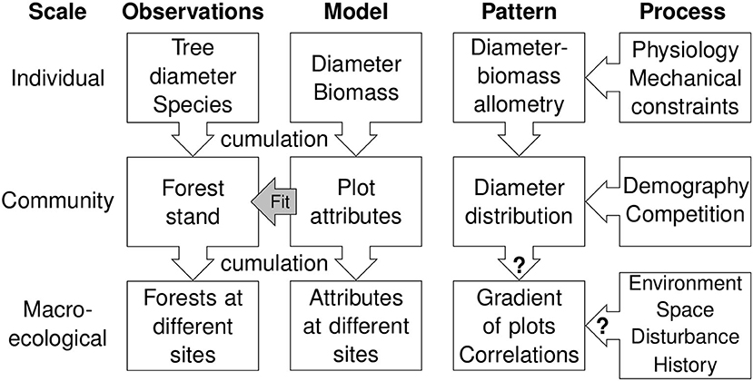
Figure 6. Conceptual view of the different patterns at different scales (from the individual to the macroecological level), the process that possibly drive these patterns, the observations from which the patterns arise, and the models to predict observations. Model analysis is used to generate an obvious pattern at macroecological level that is inherited from patterns at lower levels and assess if this obvious pattern differs from the observed one.

Spatial correlation plays a particular role in generating macroecologial patterns. An extension of the current work consists of exploring how variance in structural attributes is partitioned differently between space and environment (both considered macroecological processes) when considering original data or the deviations to the null model (Dray et al., 2006; Bauman et al., 2018).

Another possible extension of the current work is to develop null models for other patterns than the gradient of plots and correlations of structural variables, such as patterns in species relative abundances, the relationship between species diversity and forest structural attributes (Chisholm et al., 2013; Day et al., 2013), or the relationship between diversity and productivity (Liang et al., 2016). In this latter case, the “more individual” hypothesis can be seen as a null model. This hypothesis predicts that the positive relationship between productivity and species richness is inherited from the cumulation of individuals, without requiring any kind of interaction between species (Š́ımová et al., 2013; McClain et al., 2016). Deviation from the pattern predicted by the “more individual” hypothesis may then signal species interactions. On the other hand, macroecological processes may still operate while resulting in a pattern that is undistinguishable from that generated by the null model, as if these processes were neutral. Hubbell's (2001) neutral theory of species assemblage predicts patterns of species abundances that may not be distinguishable from those relying on Hutchinson's species niches. Another example is Brown et al.'s equal fitness paradigm (Brown et al., 2018) that predicts an equal energetic fitness for all species despite the diversity of life history strategies among species.

4.3. The Null Model Must Be Kept Simple and Several Options Be Tested

The choice of the model used to filter out the dominant pattern may have an influence on the results. If the parametric component is made more realistic by adding detail, at some point all the observed pattern will be predicted by the parametric component, but processes explaining site differences included in the parametric component (Gotelli and Ulrich's, 2012). Like Gotelli and Graves (1996), we reckon that the parametric component should rely only on processes operating at lower levels and be kept as simple and parsimonious as possible while still being able to generate the dominant pattern.

A sensitivity analysis using different options for the parametric component of the null model may be useful to assess the influence of model choice. In the present case, we obtained similar results when using either the exponential or the power distribution for tree dbh. The key point is the capacity of the parametric component of the null model to generate the dominant pattern (with the exponential distribution performing better than the power distribution in our study). Nevertheless, the absence of residual pattern in the deviations between observations and predictions would not necessarily mean that the null model is the pattern generating process. Competing models would be needed to assess this type II error.

4.4. Conclusions

We used inventory plots from nine tropical forest sites to perform classical analysis in ecological studies (correlation, ordination) aiming at identifying patterns in the data and inferring underlying processes. We found the expected patterns of correlation between structural variables and ordination of plots from poorly to highly stocked forests. These patterns were dominant because they prevailed over site differences, and obvious because they were inherited from the constituent elements of the forest. But they also hid site differences, i.e., the pattern of interest for ecological inference. The null model analysis revealed these site differences by filtering out the dominant patterns. We expect our conclusions to be much more general in application. It could be a clue in particular to explain why only small shares of the variation in structural attributes of tropical forests (like biomass) can be explained by environmental drivers.

Data Availability Statement

The model and analysis are implemented as R (version 3.3.2) code. All code is available in Supplementary Text 6. The data supporting the results are publicly available at doi: 10.5281/zenodo.4338387.

Author Contributions

NP designed the study and made the analyses. NP, FM, JL, GD, JRP, and SGF contributed to the writing of the manuscript. PP, JFB, TWC, and PC provided comments. GD, NA, FBB, CJC, NLEO, EF, DH, AN, JRP, BS, and SGF contributed data. FB managed data. All authors contributed to the article and approved the submitted version.

Funding

This study was supported in parts by the USDA National Institute of Food and Agriculture McIntire Stennis projects 1017711 and by the Department of Forestry and Natural Resources, Purdue University. Funding was also provided by the Funds voor Wetenschappelijk Onderzoek. FM was supported by the GAMBAS project funded by the French National Research Agency (ANR-18-CE02-0025).

Conflict of Interest

The authors declare that the research was conducted in the absence of any commercial or financial relationships that could be construed as a potential conflict of interest.

Publisher's Note

All claims expressed in this article are solely those of the authors and do not necessarily represent those of their affiliated organizations, or those of the publisher, the editors and the reviewers. Any product that may be evaluated in this article, or claim that may be made by its manufacturer, is not guaranteed or endorsed by the publisher.

Acknowledgments

We thank the Ministère des Eaux, Forêts, Chasse et Pêche (MEFCP, Central African Republic), the Institut Centrafricain de Recherche Agronomique (ICRA, Central African Republic), the University of Bangui (Central African Republic), the Société Centrafricaine de Déroulage (SCAD, Central African Republic), the Centre de coopération internationale en recherche agronomique pour le développement (CIRAD), the Service de Coopération et d'Actions Culturelles (SCAC/MAE, Central African Republic), and the Agence Française de Développement (AFD) for their logistical, administrative and funding support to the M'Baïki site. We thank the Karnataka Forest Department for permission to carry out research work in Uppangala.

Supplementary Material

The Supplementary Material for this article can be found online at: https://www.frontiersin.org/articles/10.3389/fevo.2021.599200/full#supplementary-material

References

Abdi, H., and Williams, L. J. (2010). Principal component analysis. WIRes. Computation. Stat. 2, 433–459. doi: 10.1002/wics.101

PubMed Abstract | CrossRef Full Text | Google Scholar

Baraloto, C., Rabaud, S., Molto, Q., Blanc, L., Fortunel, C., Hérault, B., et al. (2011). Disentangling stand and environmental correlates of aboveground biomass in Amazonian forests. Global Change Biol. 17, 2677–2688. doi: 10.1111/j.1365-2486.2011.02432.x

CrossRef Full Text | Google Scholar

Bastin, J. F., Rutishauser, E., Kellner, J. R., Saatchi, S., Pélissier, R., Hérault, B., et al. (2018). Pan-tropical prediction of forest structure from the largest trees. Global Ecol. Biogeogr. 27, 1366–1383. doi: 10.1111/geb.12803

PubMed Abstract | CrossRef Full Text | Google Scholar

Bauman, D., Drouet, T., Fortin, M.-J., and Dray, S. (2018). Optimizing the choice of a spatial weighting matrix in eigenvector-based methods. Ecology 99, 2159–2166. doi: 10.1002/ecy.2469

PubMed Abstract | CrossRef Full Text | Google Scholar

Brown, J. H., Hall, C. A. S., and Sibly, R. M. (2018). Equal fitness paradigm explained by a trade-off between generation time and energy production rate. Nat. Ecol. Evol. 2, 262. doi: 10.1038/s41559-017-0430-1

PubMed Abstract | CrossRef Full Text | Google Scholar

Brunck, F., Grison, F., and Maître, H. F. (1990). L'okoumé, Aucoumea klaineana Pierre. Monographie (Nogent-sur-Marne: CIRAD-CTFT)

Google Scholar

Buja, A., and Eyuboglu, N. (1992). Remarks on parallel analysis. Multivar. Behav. Res. 27, 509–540. doi: 10.1207/s15327906mbr2704_2

PubMed Abstract | CrossRef Full Text | Google Scholar

Chave, J., Andalo, C., Brown, S., Cairns, M. A., Chambers, J. Q., Eamus, D., et al. (2005). Tree allometry and improved estimation of carbon stocks and balance in tropical forests. Oecologia 145, 87–99. doi: 10.1007/s00442-005-0100-x

PubMed Abstract | CrossRef Full Text | Google Scholar

Chave, J., Réjou-Méchain, M., Búrquez, A., Chidumayo, E., Colgan, M. S., Delitti, W. B. C., et al. (2014). Improved allometric models to estimate the aboveground biomass of tropical trees. Global Change Biol. 20, 3177–3190. doi: 10.1111/gcb.12629

PubMed Abstract | CrossRef Full Text | Google Scholar

Chisholm, R. A., Muller-Landau, H. C., Abdul Rahman, K., Bebber, D. P., Bin, Y., Bohlman, S. A., et al. (2013). Scale-dependent relationships between tree species richness and ecosystem function in forests. J. Ecol. 101, 1214–1224. doi: 10.1111/1365-2745.12132

PubMed Abstract | CrossRef Full Text | Google Scholar

Couteron, P., Pélissier, R., Mapaga, D., Molino, J. F., and Teillier, L. (2003). Drawing ecological insights from a management-oriented forest inventory in French Guiana. For. Ecol. Manag. 172, 89–108. doi: 10.1016/s0378-1127(02)00310-9

CrossRef Full Text | Google Scholar

Day, M., Baldauf, C., Rutishauser, E., and Sunderland, T. C. H. (2013). Relationships between tree species diversity and above-ground biomass in Central African rainforests: implications for REDD. Environ. Conserv. 41, 64–72. doi: 10.1017/S0376892913000295

PubMed Abstract | CrossRef Full Text | Google Scholar

Dinerstein, E., Olson, D., Joshi, A., Vynne, C., Burgess, N. D., Wikramanayake, E., et al. (2017). An ecoregion-based approach to protecting half the terrestrial realm. BioScience 67, 534–545. doi: 10.1093/biosci/bix014

PubMed Abstract | CrossRef Full Text | Google Scholar

Dormann, C. F., Fründ, J., and Schaefer, H. M. (2017). Identifying causes of patterns in ecological networks: opportunities and limitations. Annu. Rev. Ecol. Evol. Syst. 48, 559–584. doi: 10.1146/annurev-ecolsys-110316-022928

CrossRef Full Text | Google Scholar

Dray, S., Legendre, P., and Peres-Neto, P. R. (2006). Spatial modelling: a comprehensive framework for principal coordinate analysis of neighbour matrices (PCNM). Ecol. Model. 196, 483–493. doi: 10.1016/j.ecolmodel.2006.02.015

CrossRef Full Text | Google Scholar

Fayolle, A., Picard, N., Doucet, J. L., Swaine, M., Bayol, N., Bénédet, F., et al. (2014a). A new insight in the structure, composition and functioning of central African moist forests. For. Ecol. Manag. 329, 195–205. doi: 10.1016/j.foreco.2014.06.014

CrossRef Full Text | Google Scholar

Fayolle, A., Swaine, M. D., Bastin, J. F., Bourland, N., Comiskey, J. A., Dauby, G., et al. (2014b). Patterns of tree species composition across tropical African forests. J. Biogeogr. 41, 2320–2331. doi: 10.1111/jbi.12382

PubMed Abstract | CrossRef Full Text | Google Scholar

Gotelli, N. J., and Graves, G. R. (1996). Null Models in Ecology. (Washington, DC: Smithsonian Institute Press)

Google Scholar

Gotelli, N. J., and Ulrich, W. (2012). Statistical challenges in null model analysis. Oikos 121, 171–180. doi: 10.1111/j.1600-0706.2011.20301.x

CrossRef Full Text | Google Scholar

Gotelli, N. J., Ulrich, W., and Maestre, F. T. (2011). Randomization tests for quantifying species importance to ecosystem function. Method. Ecol. Evol. 2, 634–642. doi: 10.1111/j.2041-210X.2011.00121.x

CrossRef Full Text | Google Scholar

Grimm, V., and Railsback, S. F. (2012). Pattern-oriented modelling: a ‘multi-scope' for predictive systems ecology. Philos. Trans. R. Soc. B Biol. Sci. 367, 298–310. doi: 10.1098/rstb.2011.0180

PubMed Abstract | CrossRef Full Text | Google Scholar

Hubbell, S. P. (2001). The Unified Neutral Theory of Biodiversity and Biogeography. No. 32 in Monographs in Population Biology (Princeton, NJ: Princeton University Press).

Google Scholar

Lawton, J. H. (1999). Are there general laws in ecology? Oikos 84, 177–192. doi: 10.2307/3546712

CrossRef Full Text | Google Scholar

Legendre, P., and Borcard, D. (2018). Box–Cox-chord transformations for community composition data prior to beta diversity analysis. Ecography 41, 1820–1824. doi: 10.1111/ecog.03498

CrossRef Full Text | Google Scholar

Legendre, P., and Legendre, L. (1998). Numerical Ecology, 2nd Edn. No. 20 in Developments in Environmental Modelling (Amsterdam: Elsevier Science).

Google Scholar

Levin, S. A. (1992). The problem of pattern and scale in ecology: The Robert H. MacArthur award lecture. Ecology 73, 1943–1967. doi: 10.2307/1941447

CrossRef Full Text | Google Scholar

Lewis, S. L., Sonke, B., Sunderland, T., Begne, S. K., Lopez-Gonzalez, G., van der Heijden, G. M. F., et al. (2013). Aboveground biomass and structure of 260 African tropical forests. Philos. Trans. R. Soc. Lond. B 368, 20120295. doi: 10.1098/rstb.2012.0295

PubMed Abstract | CrossRef Full Text | Google Scholar

Liang, J., Crowther, T. W., Picard, N., Wiser, S., Zhou, M., Alberti, G., et al. (2016). Positive biodiversity-productivity relationship predominant in global forests. Science 354;aaf8957. doi: 10.1126/science.aaf8957

PubMed Abstract | CrossRef Full Text | Google Scholar

Linting, M., van Os, B. J., and Meulman, J. J. (2011). Statistical significance of the contribution of variables to the PCA solution: an alternative permutation strategy. Psychometrika 76, 440–460. doi: 10.1007/s11336-011-9216-6

CrossRef Full Text | Google Scholar

McClain, C. R., Barry, J. P., Eernisse, D., Horton, T., Judge, J., Kakui, K., et al. (2016). Multiple processes generate productivity–diversity relationships in experimental wood-fall communities. Ecology 97, 885–898. doi: 10.1890/15-1669.1

PubMed Abstract | CrossRef Full Text | Google Scholar

Muller-Landau, H. C., Condit, R. S., Harms, K. E., Marks, C. O., Thomas, S. C., Bunyavejchewin, S., et al. (2006). Comparing tropical forest tree size distributions with the predictions of metabolic ecology and equilibrium models. Ecol. Lett. 9, 589–602. doi: 10.1111/j.1461-0248.2006.00915.x

PubMed Abstract | CrossRef Full Text | Google Scholar

Palla, F., Picard, N., Abernethy, K. A., Ukizintambara, T., White, E. C., Riéra, B., et al. (2011). Structural and floristic typology of the forests in the forest-savanna mosaic of the Lopé National Park, Gabon. Plant Ecol. Evol. 144, 255–266. doi: 10.5091/plecevo.2011.478

CrossRef Full Text | Google Scholar

Peh, K. S. H., Lewis, S. L., and Lloyd, J. (2011). Mechanisms of monodominance in diverse tropical tree-dominated systems. J. Ecol. 99, 891–898. doi: 10.1111/j.1365-2745.2011.01827.x

CrossRef Full Text | Google Scholar

Peres-Neto, P. R., and Legendre, P. (2010). Estimating and controlling for spatial structure in the study of ecological communities. Global Ecol. Biogeogr. 19, 174–184. doi: 10.1111/j.1466-8238.2009.00506.x

CrossRef Full Text | Google Scholar

Poulsen, J. R., Clark, C. J., and Palmer, T. M. (2013). Ecological erosion of an Afrotropical forest and potential consequences for tree recruitment and forest biomass. Biol. Conserv. 163, 122–130. doi: 10.1016/j.biocon.2013.03.021

CrossRef Full Text | Google Scholar

Rivière, L. (1992). Étude de l'évolution des peuplements naturels d'okoumé (Aucoumea klaineana Pierre) dans le sud-estuaire du Gabon. Construction de tables de croissance provisoires. Thèse de doctorat, Université Paris 6, Paris

Google Scholar

Rollet, B. (1974). L'architecture des forêts denses humides sempervirentes de plaine (Nogent-sur-Marne: CTFT).

Google Scholar

Sellan, G., Simini, F., Maritan, A., Banavar, J. R., Haulleville, T., Bauters, M., et al. (2017). Testing a general approach to assess the degree of disturbance in tropical forests. J. Veg. Sci. 28, 659–668. doi: 10.1111/jvs.12512

CrossRef Full Text | Google Scholar

Šímová, I., Li, Y. M., and Storch, D. (2013). Relationship between species richness and productivity in plants: the role of sampling effect, heterogeneity and species pool. J. Ecol. 101, 161–170. doi: 10.1111/1365-2745.12011

CrossRef Full Text | Google Scholar

Wiegand, T., Jeltsch, F., Hanski, I., and Grimm, V. (2003). Using pattern-oriented modeling for revealing hidden information: a key for reconciling ecological theory and application. Oikos 100, 209–22. doi: 10.1034/j.1600-0706.2003.12027.x

CrossRef Full Text | Google Scholar

Zanne, A. E., Lopez-Gonzalez, G., Coomes, D. A., Ilic, J., Jansen, S., Lewis, S. L., et al. (2009). Global wood density database. Dryad Dig. Repository. doi: 10.5061/dryad.234

CrossRef Full Text | Google Scholar