Anthropogenic Induced Beta Diversity in Plant–Pollinator Networks: Dissimilarity, Turnover, and Predictive Power

Introduction

As human dominance of the biosphere continues to grow, two landscape types are continuing to expand: agricultural and urban systems (Foley et al., 2005; Seto et al., 2010). While agricultural ecosystems have been extensively studied, and the negative effects of agricultural intensification on species and ecological processes are relatively well understood (IPBES, 2018), it is only in the last two decades that attention has turned to urban ecosystems (McPhearson et al., 2016).

Urban landscapes can negatively affect many species, with species richness tending to be lower in urban landscapes (Shochat et al., 2006; Grimm et al., 2008; McKinney, 2008). Yet, urban adapted species can thrive, occurring at high levels of abundance (Shochat et al., 2010) and there is accumulating evidence that the urban landscape is driving convergent phenotypic changes (Alberti et al., 2017a,b), suggesting that cities impose similar evolutionary selective regimes (Santangelo et al., 2018). Urban areas can potentially act as a refuge for species (Carrier and Beebee, 2003; Menke et al., 2011; Hall et al., 2017), with gardens and public space recognized as important conservation arenas (Goddard et al., 2010). Furthermore, effects are not uniform across either urban or agricultural landscapes but vary with intensity. While previous reviews of urban gradients have indicated that species richness follows a hump shaped curve along an urban gradient, with species richness peaking at medium levels of urban intensity (Blair, 1999; Germaine and Wakeling, 2001; McKinney, 2002; Shochat et al., 2006), a more recent global meta-analysis has indicated that increasing intensity of urbanization continually erodes species richness when compared to natural habitats (Newbold et al., 2015). Newbold et al. (2015) found a similar pattern and magnitude of species loss for increasing intensity of crop and pastoral agriculture and plantation silviculture, indicating that land use intensification in general reduces local species richness (Gerstner et al., 2014; Beckmann et al., 2019). Yet, the response of any species to increasing land use intensity can be specific to the land use and the species’ functional traits (Rader et al., 2014). For example, while agricultural intensification and urbanization are both associated with decreases in pollinating species diversity (Le Féon et al., 2010; Bates et al., 2011), more recently urban landscapes have been suggested as a potential refuge for bees, but not other insect pollinator groups, from the surrounding agricultural matrix (Banaszak-Cibicka and Żmihorski, 2012; Hall et al., 2017).

Moving beyond local species richness, beta diversity measures the compositional turnover of species among communities. Higher beta diversity means that two communities have dissimilar compositions, are heterogenous, while low beta diversity implies that communities are homogenous. There is building consensus that beta diversity declines with agricultural intensification, meaning that communities in intensive agricultural landscapes undergo homogenization, although the trend is not universal and depends on the group studied (Vellend et al., 2007; Ekroos et al., 2010; Flohre et al., 2011; Karp et al., 2012). Similarly, urban landscapes have the most homogenized communities of any studied land use types in a global meta-analysis (Newbold et al., 2015), providing evidence for the claim that urbanization results in biotic homogenization (McKinney, 2006).

Yet the impacts of land use change and intensification, particularly urbanization, on ecosystem processes such as species interactions are less well understood (Shochat et al., 2006; Alberti, 2010; Elmqvist et al., 2015; but see Baldock et al., 2015). Pollination is emerging as a model system for studying the effects of global change on species interactions due to a large literature on mechanistic aspects of pollination (Harrison and Winfree, 2015) and well-developed network science tools to visualize and parameterize interaction webs (Dunne, 2006; Bascompte and Jordano, 2013). Pollinators have been extensively studied in agricultural systems and natural habitats (Kremen et al., 2002; Ricketts et al., 2008; Potts et al., 2010), and while there is a growing literature on pollinators in urban landscapes (Cane et al., 2006; Bates et al., 2011; Geslin et al., 2013; Fortel et al., 2014; Baldock et al., 2015; Theodorou et al., 2017), it remains an under-studied area, particularly in terms of describing the patterns of interaction beta diversity. Trøjelsgaard et al. (2015) studied interaction network beta diversity across the Canary Islands, finding strong spatial structuring of the networks, yet, to our knowledge, no study has explored the patterns of interaction beta diversity in anthropogenic landscapes.

Anthropogenic disturbances affect beta diversity through multiple processes. First, when disturbances decrease species richness, beta diversity can increase. This is because the probability that sites do not share species increases when fewer species occupy each site (Chase et al., 2011). Second, disturbances can impose similar ecological filters over vast areas (Keddy, 1992), thereby homogenizing communities (Karp et al., 2012), or create environmental heterogeneity, thereby diversifying communities (Hawkins et al., 2015). Increasing community dissimilarity with increasing geographical distance, known as distance decay, is well documented for single trophic communities (e.g., Nekola and White, 1999). More recently, distance decay has been shown to occur at both local and regional scales for plant–pollinator interaction networks (Carstensen et al., 2014; Simanonok and Burkle, 2014; Trøjelsgaard et al., 2015).

Here, we first quantify the spatial and anthropogenic induced turnover in plant–pollinator interaction networks by examining the beta diversity of species and interactions between network pairs across 21 sites. We assume that the environment is composed of both its landscape context (agricultural vs. urban) and the intensity of the land use (high, medium, or low). At the spatial scale of this study (50 km), we predict that the anthropogenic gradient dissimilarity, created by combining an urban and agricultural gradient, will produce stronger community and interaction dissimilarity than distance decay effects.

Second, we quantify the components of interaction turnover which drive network difference. Rewiring, the reassembly of interactions among co-occurring species, and species driven interaction turnover, interactions between species conditioned by their co-occurrence (Pellissier et al., 2018), are the major components of interaction turnover. Species turnover can be further decomposed into its three components: plant-driven, pollinator-driven, and plant-and-pollinator driven turnover. Each component of species driven turnover is due to compositional turnover of the interacting species: for example, where a plant species is present at site A but absent from a site B, any interaction the plant is involved in will turnover due to plant driven turnover in the site pair comparison A-B. The overwhelming importance of species turnover for pollination network dissimilarity (Simanonok and Burkle, 2014; Trøjelsgaard et al., 2015) suggests that we are likely to find that rewiring is a minority contributor to network dissimilarity across the 21 sites of our study region. Further, we explore how the components of species driven interaction turnover are impacted by spatial distance and anthropogenic landscapes by decomposing species driven interaction turnover into its three components and regressing them against spatial distance and anthropogenic induced environmental dissimilarity.

Finally, if we are to move beyond descriptive studies of interaction biogeography, we must understand the variables that are predictive of interaction turnover. We explore the factors predictive of interaction turnover, aiming to understand whether there is predictive power in broad landscape, network, and ecological variables or whether species specific information is required for accurate predictions. Requiring species specific information would mean much more intensive data collection on species traits is needed to build a predictive biogeography of interactions. We train a model to predict turnover using a combination of interaction properties, relative floral abundances, spatial distance, and anthropogenic environmental dissimilarities, and then test its predictive performance against models containing species as random effects to determine the source of predictive power for interaction turnover.

Thus, our aims are threefold, sequential and complementary: explore the (1) patterns, (2) components, and (3) predictive variables generating beta diversity in interaction networks situated in anthropogenic landscapes.

Materials and Methods

Field Site Selection

Twenty-one sites were sampled around east Leinster, Ireland, along gradients of agricultural intensity, urbanization, and semi-naturalness (Figure 1). The agricultural and urban sites were located along gradients of intensity; high, medium, and low, with three sites to each level for replication, while there was a single semi-natural level containing three sites. Each site is characterized by the degree of urbanization, measured as the percentage of impervious surface in the landscape, agricultural intensity, measured as the average field size in the landscape, and the percentage of semi-natural vegetation. The low urban and semi-natural sites were not exclusively urban or semi-natural, both containing agricultural land, due to the impossibility of finding exclusively low urban or semi-natural landscapes in the east Leinster region. The site characteristics are shown in Supplementary Table S2. A minimum distance of 1km separated all sites, to ensure that a separate pollinator community was sampled at each site.

FIGURE 1

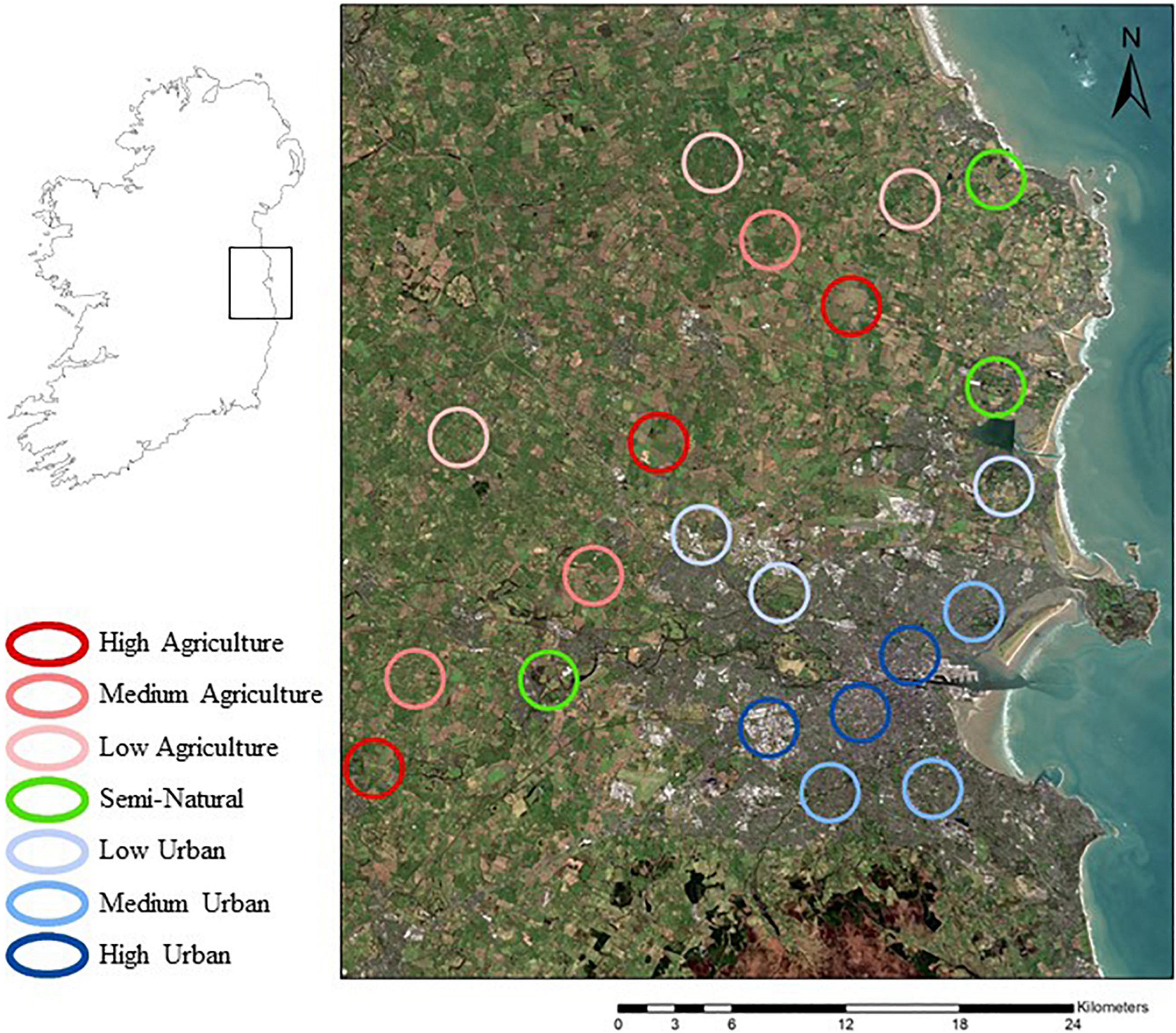
Figure 1. Location of the 21 sites. The nine urban sites are in Dublin city. The nine agricultural sites are in the surrounding agricultural landscape in counties Dublin, Kildare, and Meath and the three semi natural sites are in landscapes with a higher proportion of semi natural meadows.

The urbanization gradient was created using an impervious surface index, from a impervious surface map generated by the Copernicus Pan European Land Service¹ [© European Union, Copernicus Land Monitoring Service 2018, European Environment Agency (EEA)], while the agricultural gradient was created using an index of average field size (Supplementary Table S1). Each index was calculated over an area within a 1.5 km radius circle, with this circle delimiting the boundary of a “site.” Sites categorized as “high” urbanization have 70–74% impervious surface, those as “medium” urbanization have 42–46%, and those as “low” urbanization have 12–18%. To calculate average field size, the number of fields in a 1.5 km radius circle at candidate sites were counted using Google Maps My Maps application² which was then divided by the area under agriculture obtained from the Copernicus Urban Atlas land use map³ [© European Union, Copernicus Land Monitoring Service 2018, European Environment Agency (EEA)], to obtain the average field size at that site. Both arable and pasture were considered agricultural land. An average field size of greater than 5 hectares (5.0–6.5 ha) within a circle of 1.5 km radius was considered a high intensity agricultural landscape, between 3.5 and 5 ha (3.8–4.4 ha) medium intensity and less than 3.5 ha (2.5–3.5 ha) average field size a low intensity agricultural landscape (Supplementary Table S1).

Average field size was used as the agricultural intensity index instead of area under agriculture as average field size is a more independent measure of the intensity of agricultural activities. Arable farmers remove field boundaries to create larger fields for more efficient use of machines and intensive pasture, such as dairying, remove field boundaries for more flexible paddock management with temporary electrical fences. There is a trend of increasing area under agriculture along the agricultural index based on field size, mostly due to the larger amounts of field boundaries at lower average field sizes, yet we chose to use field size as opposed to area under agriculture to more in independently sample intensity of agricultural landscapes. The semi-natural index is designed to measure landscapes which have a lower area under agriculture, where semi-naturalness is measured as the percentage of semi-natural vegetation in a 1.5 km radius.

Semi natural sites were categorized as those with greater than 10% of the site area being under semi natural meadow grassland. Semi natural vegetation was calculated by combining the Herbaceous Vegetation Associations category of land use in the 2012 Copernicus Urban Atlas land use map⁴, plus the habitats surveyed in the Grasslands of Ireland study⁵.

Sampling Flowers, Flower–Visitors, and Flower–Visitor Interactions

Each of the 21 sites was sampled four times between 5 May and 20 August 2018 at monthly intervals. Plants and pollinators were sampled along a 2 m × 1 km transect within each 1.5 km radius site, with sub-sections of the transect allocated proportionately to all land cover types comprising more than 1% of the selected site (e.g., pasture, arable, continuous urban fabric; see Supplementary Figure S1 legend). Transects in residential areas were positioned along the boundary between pavements and residential gardens, so that 1 m of the transect width was located in gardens and the other 1 m was located on pavements and road verges. Transect locations were chosen using a random number generator to select points from a grid, and transect sections were located as close as possible to those points. Where land cover types were particularly dominant within a site, a maximum transect section length of 250 m was walked, with multiple transects of the same land cover walked across multiple locations. The amount of pasture and arable land surveyed at each agricultural site is shown in Supplementary Table S4.

Flowers were sampled by noting every flowering species on the outward walk of the transect and then counting the floral units of each species on the return walk. A floral unit was defined as an individual flower or collection of flowers that an insect of 5 mm body length could walk between (see Baldock et al., 2015, Supplementary Table S5) and comprised a single capitulum for Asteraceae, a secondary umbel for Apiaceae and a single flower for most other taxa. Grasses, sedges and wind-pollinated forbs were not sampled.

Flower–visitor interactions were quantified by walking along each transect and recording every insect on flowers up to 1m either side of the transect line to a height of 2 m, where appropriate, e.g., along hedgerows. An attempt was made to net all bees and hoverflies (Syrphidae), which were frozen and later identified to species. All other flower visiting insects were recorded at the family level (Coleoptera, Diptera, Lepidoptera). Bees and hoverflies were identified using Stubbs and Falk (2002) and Falk (2015) respectively, with identifications checked by taxonomists (see Acknowledgments). Plants were identified using Rose and O’Reilly (2006) and the phone application Plantnet⁶, 85% to species and the rest to genus or morpho species. Sampling for flower visitors and their interactions took place between 09:00 and 19:00 h on dry, warm, non-windy days. No sampling took place on days that were below 12°C or above Beaufort scale of 5 (fresh breeze). Two sites were sampled each day, one in the morning and one in the afternoon. The 21 sites were sampled over a 2-week period each month, with the order of sites being sampled each month chosen randomly. Environmental conditions such as temperature, wind strength, cloudiness, sunshine, habitat, and vegetation structure were recorded for each section of the transect and are made available on the figshare data repository (see section “Acknowledgments”).

Community and Network Dissimilarity

The level of pairwise dissimilarity between networks was calculated using the recently developed network diversity indices that take advantage of Hill numbers (Ohlmann et al., 2019). Pairwise network beta diversity was calculated using the disPairwise function of the R package econetwork (Dray et al., 2020a). For the equations used in the disPairwise function see the Supplementary Materials section “Calculating beta diversity of interaction networks” and Ohlmann et al. (2019). To ensure comparability between network beta diversity measures and plant and pollinator community beta diversity measures, Hill numbers were used to calculate the plant and pollinator community pairwise beta diversity (see function hill_taxa_parti_pairwise in package hillR; Li, 2018).

Communities differing in species or interaction richness are likely to be less similar than communities of equal richness (Anderson et al., 2011; Burkle et al., 2016). The influence of different alpha diversities was mitigated by using a null model based on 1000 random assignments of species and interactions to our networks according to a probability distribution derived from their actual occurrences across the sites (Trøjelsgaard et al., 2015; Pellissier et al., 2018). That is, widespread species were more likely to be drawn and assigned to a network during the random assortments, and numbers of species and interactions assigned to a random network were constrained to equal empirical numbers. Across all pairwise combinations, we calculated the empirical similarity in plant, pollinator, and interaction composition (βempirical). The deviation from randomness was measured using z-scores given as (βempirical -mean(βresampled))/SDresampled, where mean(βresampled) and SDresampled are the mean and standard deviation of the similarities achieved from the 1000 random assortments of species and interactions. Hence, a positive z-score suggests that two communities are more similar than expected if species or interactions were distributed randomly across the region, and vice versa for a negative z-score. The significance level of each βempirical value was obtained using the resampled values as a benchmark and all βempirical values having z-scores larger than 1.96 or smaller than -1.96, respectively, were deemed significantly different (p < 0.05) from random.

Custom R functions create null interaction networks across sites is available on GitHub at: https://github.com/ciwhite/network_beta_diversity. The null models were tested on simulated community and interaction network data to confirm that the randomization procedure could detect both the absence and presence of beta diversity patterns.

A variance partitioning exercise was performed to assess the level of spatial autocorrelation between the beta diversity metrics (beta diversity of the plant community, pollinator community, and interaction networks) and the environmental dissimilarity metric. Variation in communities and interaction networks was partitioned into the purely spatial, purely environmental and the spatially structured environment components. To our knowledge, this is the first-time variation partitioning has been carried out on interaction networks.

Both the empirical beta diversity similarity values and the derived z-scores were regressed against geographical distance and anthropogenic induced environmental dissimilarity using Mantel tests with 1000 permutations performed with the vegan v. 2.0-8 package for R (Oksanen et al., 2019). Anthropogenic induced environmental dissimilarity (hereafter environmental dissimilarity) is measured as the Euclidean dissimilarity of the site characteristics (agricultural intensity, urbanization, semi-naturalness) and thus describes how different a site is from another in landscape composition and intensity of use. Multi-scale moran eigen vector maps were created using the adespatial package (Dray et al., 2020b) and variation partitioning was carried out using vegan.

Components of Interaction Turnover

Here, we use the method proposed by Novotny (2009) to partition network dissimilarity into additive components of rewiring and species driven interaction turnover, as the method proposed by Poisot et al. (2012) can underestimate species turnover and overestimate rewiring (Fründ, 2021). Interactions turnover due to rewiring and species driven interaction turnover, the latter of which is due to changes in species composition and can be further partitioned into plant driven, pollinator driven and plant + pollinator driven turnover. More formally, if 1 and 2 are two ecological networks, then let I_rewired be the number of interactions that change between the shared species of 1 and 2, and let I_species be the number of interactions that change due to changes in species composition (Figure 2). The total number of interactions that differ between A and B is then given by I_rewired + I_species, and the proportion of turnover that is due to rewiring and species-driven interaction turnover are: rewiring = I_rewired/(I_rewired + I_species) and species-driven = I_species/(I_rewired + I_species).

FIGURE 2

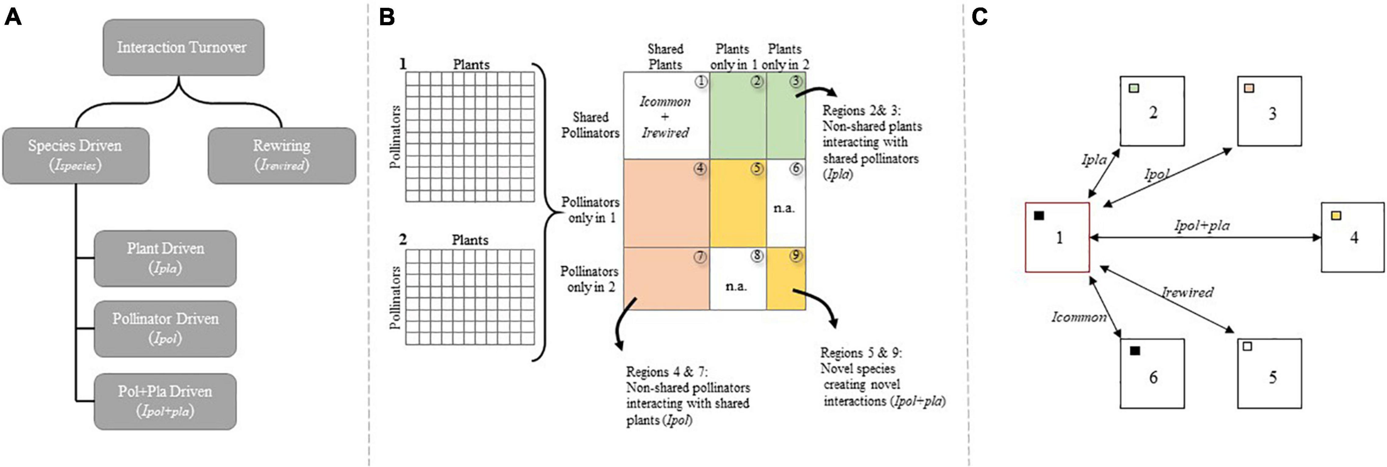
Figure 2. (A) Interaction turnover between two ecological networks can be partitioned into contributions from rewiring (i.e., when shared species alter their interactions; I_rewired) and species-driven turnover (i.e., when changing species composition change interactions; I_species), with the latter being further partitioned into pollinator-driven (I_pol), plant-driven (I_pla) and pollinator + plant-driven (I_pol+pla) interaction turnover. (B) Matrices 1 and 2 represent ecological networks, with pollinator species arranged in rows and plant species in columns, which are artificially merged into one large matrix in order to identify interactions contributing to the different categories of interaction turnover. Region 1 contains interactions between shared species, and I_common denotes interactions found in both 1 and 2, whereas I_rewired is the sum of interactions only observed in either matrix 1 or 2, but between shared species. Shaded areas contain interactions contributing to species–driven interaction turnover. Interactions located in regions 2 and 3 are between shared pollinators and non-shared plants (i.e., the plants are found in either matrix 1 or 2 but not both) and represent plant–driven interaction turnover. Interactions located in regions 4 and 7 are between shared plants and non-shared pollinators comprising the pollinator-driven interaction turnover. Finally, regions 5 and 9 contain interactions between non-shared pollinators and non-shared plants and comprise the pollinator + plant–driven interaction turnover. Regions marked with n.a. do not contain any interactions due to the artificial merging of matrices 1 and 2. (C) Interaction specific site-pair combinations. This (hypothetical) interaction is observed at sites 1 and 6 (filled squares) while the species pair is also present at site 5, however, without interacting (open square). The plant species is absent from site 2 (green square), the pollinator species absent from site 3 (red square) and both species absent from site 4 (yellow square) allowing a dataset to be created to document all the ways in which interaction networks differ. Six site-pair combinations are possible in this case; 1↔5 rewiring, 1↔2: plant driven interaction turnover, 1↔3 pollinator driven interaction turnover, 1↔4 plant and pollinator driven interaction turnover and 1↔6: no interaction turnover (interaction constancy). Figure adapted from Trøjelsgaard et al. (2015).

Species–driven interaction turnover (I_species) can be further partitioned into that caused by (i) pollinators only present in one of the networks but interacting with plants present in both (i.e., pollinator–driven interaction turnover, I_pol), (ii) plants only present in one of the networks but interacting with pollinators present in both (i.e., plant–driven interaction turnover, I_pla), or (iii) plants and pollinators only occurring in one of the communities and interacting together (i.e., a complete turnover of species and hence interactions, I_pol+pla) (Figure 2). Therefore, if I_pla is the number of interactions between non-shared plants and shared pollinators (regions 2 and 3 in Figure 2), I_pol is the number of interactions between non-shared pollinators and shared plant species (regions 4 and 7 in Figure 2), and I_pol+pla is the number of interactions between non-shared pollinators and non-shared plants (regions 5 and 9 in Figure 2), then I_species = I_pol + I_pla + I_pol+pla, and the fractions of the species-driven interaction turnover that can be explained by replacement of pollinators, plants or both are T_pol = I_pol/I_species; T_pla = I_pla/I_species and T_pol+pla = I_pol+pla/I_species, respectively. Custom R functions to partition interaction turnover into the various components are available on GitHub at: https://github.com/ciwhite/network_beta_diversity.

We used Local Regression (loess) to account for non-linearities in the relationship between both plant driven (T_pla) and pollinator driven (T_pol) interaction turnover and each of geographical or anthropogenic environmental distance. Loess was evaluated with confidence intervals calculated using bootstrap with replacement (Wehrens et al., 2000). First, we estimated a local regression for the empirical data and local regressions for each of 10 000 permutations of the data. Second, “basic bootstrap confidence intervals” (Wehrens et al., 2000) were calculated.

Predicting Interaction Turnover

Our aim was to explore whether it is possible to predict interaction turnover due to rewiring, plant driven turnover, pollinator driven turnover and plant and pollinator driven turnover. In particular, we are interested in where the main sources of predictive power lie: can we predict interaction turnover using site characteristics and network properties, or is information at species level required?

To do so we explore the predictive ability of three models (1) a generalized linear model (GLM) with measured ecological, landscape and network variables (detailed below), (2) a generalized linear mixed effects model (GLMM) with the measured variables as fixed effects and random effects for each plant and pollinator species involved in the interaction, and (3) a random effect GLMM containing the plant and pollinator species as random effects. The purpose of the random effects GLMM is to account for the variation contained at the species level and so by comparing the predictive power of the random effects glmm (3) to mixed effects glmm (2), we can determine whether the predictive power comes from species specific information that we have not measured or the measured ecological, landscape and network variables. Importantly, the dataset and hence species in the random effects model and the mixed effects model are the same, the random effect levels are consistent between models, allowing valid model comparisons.

Thus, for each component of interaction turnover, we explore the predictive power of three models:

$$\begin{array}{c}glm(turnover\sim ecologicalvariables+landscapevariables+\hfill \\ \hfill networkvariable,family=binomial(link=\mathrm{"}logit\mathrm{"}))\end{array}(1)$$

$$\begin{array}{c}glmm(turnover\sim ecologicalvariables+landscapevariables+\hfill \\ \hfill networkvariable+\left(1|pol\right)+\left(1|pla\right),\\ \hfill family=binomial(link=\mathrm{"}logit\mathrm{"}))\end{array}(2)$$

$$\begin{array}{c}glmm(turnover\sim (1|pol)+(1|pla),\hfill \\ \hfill family=binomial(link=\mathrm{"}logit\mathrm{"}))\end{array}(3)$$

To create the datasets for each component of interaction turnover, we first isolated each unique interaction between a plant and a pollinator species. We then noted each site pair where the interaction was constant, where the interaction rewired, where the interaction turned over due to plant driven turnover, pollinator driven turnover, or plant and pollinator driven turnover, and finally where the interaction was absent from both sites even though the species co-occurred in the site pair. Thus, for each unique interaction, we obtained every event of interaction turnover, constancy, or absence between site pairs. This dataset was split into four for each component of interaction turnover, a rewiring dataset, a plant driven turnover dataset, a pollinator driven turnover dataset and a plant and pollinator driven turnover dataset. The three models above are then applied to each dataset and their predictive power compared.

The measured ecological variables are origin of plant species (native or introduced) and a floral abundance variable measuring the difference in floral abundance between the site pair. Four different indices of floral abundance were tested in an exploratory model: the difference in floral abundance, relative difference in floral abundance and the absolute values of both. While each floral abundance variable was significant, the absolute difference in relative floral abundance proved to be most significant. As the mixed effects GLMMs would not converge when all four floral abundance variables were added, the most significant predictor, absolute difference in relative abundance, was chosen to represent the floral abundance variable. Absolute difference in relative abundance was calculated as such: for a given interaction specific site-pair combination we calculated the difference in flower abundance for the plant species involved in the interaction. This was then divided by sum of the floral abundance at both sites for that species to get a measure of the relative change in flower abundance. The absolute value of the relative change was taken and used as a predictor variable.

Four measured landscape variables were tested: (1) the environmental dissimilarity between the site pair, (2) the average agricultural intensity index of the site pair, (3) the average urbanization score of the site pair, and (4) the geographical distance between the site pair. The average of the agricultural and urbanization scores were used in addition to the environmental dissimilarity to assess whether there are directional effects of the agricultural and urban gradient respectively. Averages were used rather than differences as differences remove the directional effect of each gradient, while sums and averages are equivalent predictor variables.

Finally, the network variable was the average interaction frequency between the plant and pollinator species. Interactions with high frequency can be interpreted as linking species with high mutual affinity, such species would likely interact with high frequency if no temporal or spatial constraints are imposed (Carstensen et al., 2014). Thus, we expect interactions with high average interaction frequency to rewire less frequently, show high constancy across sites, while those with low average frequency to rewire more frequently. Average interaction frequency is the average abundance of an interaction, calculated as the sum of the interaction frequencies between two species across all sites in which they co-occur divided by the number of sites where both species co-occur (interacting or not).

Importantly, these variables should not be considered an exhaustive set, rather they represent a set that can be obtained during standard ecological network data collection. We are interested in exploring the predictive power of each model type to assess whether additional species level information needs to be collected to explain the components of interaction turnover. Each variable was scaled and centered around 0 to ensure that the GLMMs would converge.

Predictive power was measured by carrying out a model training and test exercise, where the ability of each model trained on a training dataset was used to predict interaction turnover on a test dataset. The training and test dataset are created by splitting collected dataset into non-overlapping test and training sets, meaning this is an out of sample prediction exercise. The comparator of predictive power is the area under the receiver operating curve (ROC), which is created by plotting the true positive rate (TPR) against the false positive rate (FPR) at various threshold settings. For a given threshold value, the closer the corresponding point in the ROC space is to the upper left angle (FPR = 0, TPR = 1), the greater the model’s predictive power. Thus, an indication of the overall model performance is given by the Area Under Curve (AUC) index (Hanley and McNeil, 1982). AUC is computed by numerical integration of the curve f = TPR(FPR), with values closer to 1 indicating greater model performance. By comparing the AUC values generated from the three models for each component of interaction turnover it is possible to assess the importance of routinely collected variables in ecological network studies and the species level information as contained in the random effects (For further information on the size of the test and training datasets, the specific variables used in to predict each component of interaction turnover and on model development, validation and fitting see Prediction of Interaction Turnover of the Supplementary Materials).

During the GLMM model validation procedure, the residuals were checked for overdispersion with respect to each model predictor and the discretized response using the DHARMa package (Hartig, 2020). It was found that the model was over dispersed with respect to the discretized model predictions. As such, the model behaves differently as the probability of an interaction turning over increases: the model predictions have a higher variance at high probability of interaction turnover while having a lower variance at low probability of interaction turnover. Such overdispersion is likely due to the model missing an informative predictor that was not measured in this study. The simpler binomial GLM without random effect variables did behave better in terms of overdispersion, but the simpler model’s fit prediction performance tended to be much lower than the more complex binomial GLMM. We choose to present the results of the binomial GLMM, noting that the overdispersion with respect to the discretized predictions is likely to be caused by a missing predictor variable.

Linear binomial mixed models were performed with the packages lme4 v. 1.0-5 for R (Bates et al., 2015) and all analyses were performed using R version 4.0.2. (R Core Team, 2020). We acknowledge that the linear mixed models only account for the taxonomic non-independence (i.e., the multiple entries of each species) and not necessarily the spatial non-independence (i.e., the multiple entries of the pairwise comparisons of the networks).

Results

A total of 4,161 insect flower visitors were sampled from the 21 sites, of which 62% were Hymenoptera, 35% Diptera, 2% were Lepidoptera and 1% were Coleoptera. This comprised of 85 visitor taxa (44 Diptera, 30 Hymenoptera, 11 Lepidoptera; Coleoptera were not identified beyond order) visiting 213 plant taxa (180 identified to species, 21 to genus and 12 to morpho species). A total of 862 unique interactions were recorded, resulting in a 73% sample coverage for interactions; 86 pollinator species were recorded with a 99% sampling coverage; and 192 plant species were recorded with a 97% sampling coverage (Supplementary Figure S2).

Community and Network Dissimilarity

Taking alpha diversity into account by using z-scores, geographical distance increased the pairwise dissimilarity of pollinator communities (Mantel test with 999 permutations: r_M = 0.1909, p = 0.024) and interaction networks (r_M = 0.1876, p = 0.025) but not plant communities (Mantel test with 999 permutations: r_M = 0.1338, p = 0.091; Figures 3A–C). Moreover, we found a stronger and significant increase in dissimilarity with the anthropogenic gradient dissimilarity for plants (Mantel test with 999 permutations: r_M = 0.571, p < 0.001) and interaction networks (Mantel test with 999 permutations: r_M = 0.5705, p < 0.001) (Figures 3E,F) but no impact on the pollinator communities (Mantel test with 999 permutations: r_M = 0.0934, p = 0.208) (Figure 3D). Therefore, geographically close networks and pollinator communities, but not plant communities, were more similar in their composition than expected from a random assortment of species and interactions, while distant communities or networks were no more different in their composition than expected. In contrast, plant community composition and interaction networks responded more strongly to environmental dissimilarity than geographical distance: those plant communities and interactions networks that had low environmental dissimilarity were more similar in their composition than expected under random assortment. There was no impact of the anthropogenic dissimilarity on the pollinator communities.

FIGURE 3

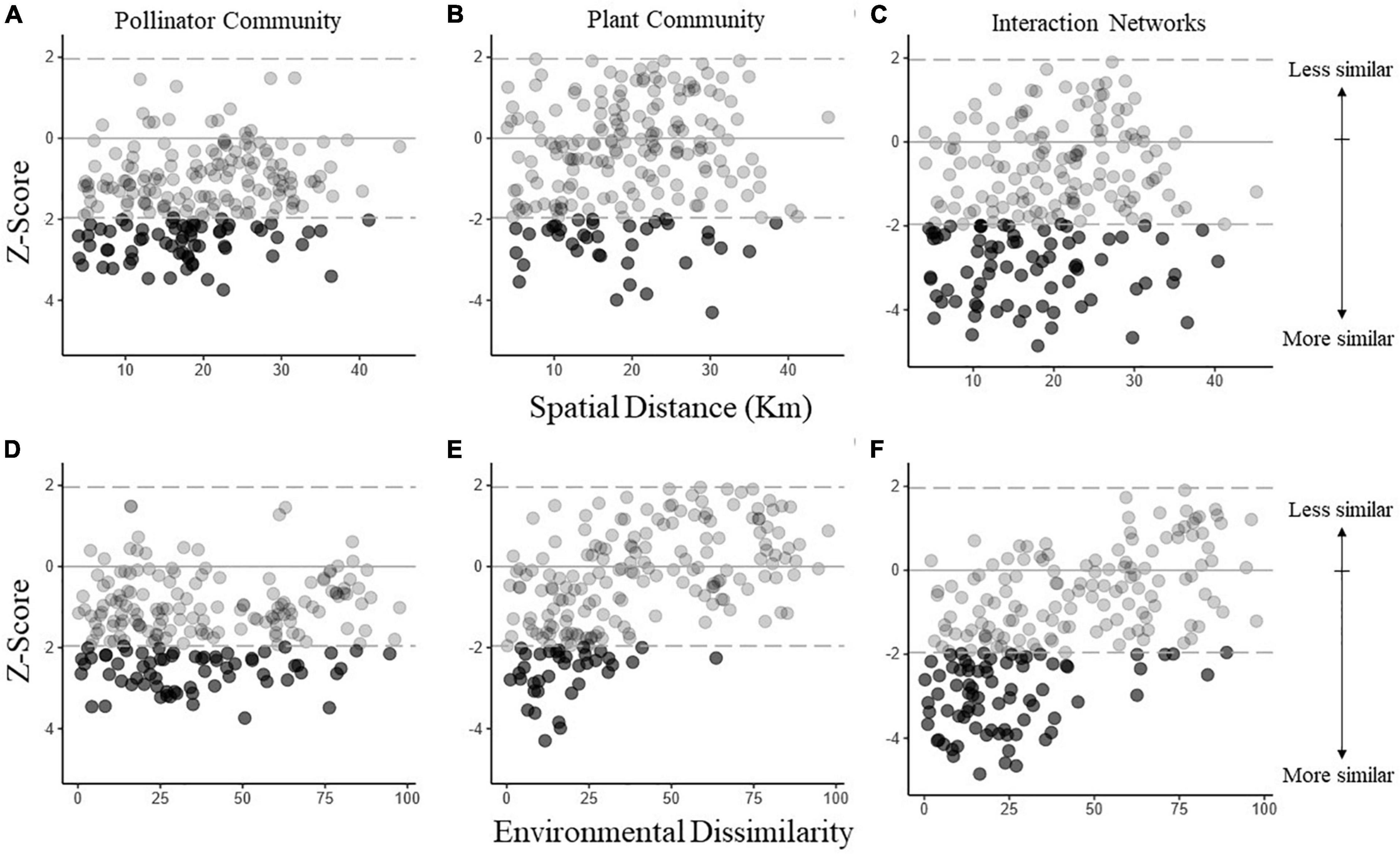
Figure 3. Dissimilarity in the composition of pollinators (A,D), plants (B,E), and their interactions (C,F) networks as a function of spatial (A–C) and environmental distance (D–F). To reduce the effect of differing α diversities, we calculated z-scores as a measure of deviation from randomness. Z-scores were given as (β_emperical – mean(β_resampled))/SD_resampled, where β_emperical is the empirical similarity between two networks, mean(β_resampled) and SD_resampled are the mean and standard deviation of the similarities when performing 1000 random assortments of species and interactions, respectively. Positive and negative z-scores signify higher and lower similarity, respectively, than expected from random distributions of species and interactions. Filled circles indicate that a given empirical pairwise comparison differed significantly from the resampled values, and gray dashed lines mark the boundary between 1.96 and -1.96.

Disaggregating the pollinator community shows that the bee community did not respond to either geographical distance or environmental dissimilarity, while hoverfly composition only responded to spatial distance (Mantel test with 999 permutations: r_M = 0.1796, p = 0.016; Supplementary Figure S8). Similarly, disaggregating the plant community into introduced and native plant species revealed that the native plant community responded to both geographical distance (Mantel test with 999 permutations: r_M = 0.2643, p = 0.002), and anthropogenic environmental dissimilarity (Mantel test with 999 permutations: r_M = 0.3486, p = 0.001; Supplementary Figures S9A,B), while the introduced plant community composition did not significantly respond to geographical distance (Mantel test with 999 permutations: r_M = 0.031, p = 0.367) but did respond to anthropogenic environmental dissimilarity (Mantel test with 999 permutations: r_M = 0.1989, p = 0.027; Supplementary Figures S9C,D).

Variation partitioning produced qualitatively similar results (see Supplementary Figure S10), where the environment partition accounted for the largest source of explained variation for each community and the networks, confirming that, in a heavily modified region, it was the anthropogenic environmental variables that structured communities more than spatial distance.

Components of Interaction Turnover

Species driven interaction turnover was the dominant component of network difference (I_species > I_rewire), accounting for ∼80% of interaction turnover (Figure 4A). The proportion of interactions that turnover due to species driven turnover and rewiring varied inversely with environmental dissimilarity; with the species driven turnover proportion increasing with increasing environmental dissimilarity (Mantel test with 999 permutations: r_M = 0.5632, p < 0.001), while the rewiring proportion decreased (–0.5632, p < 0.001; Figure 4D). There was no significant effect of spatial distance on the contribution of turnover (Mantel test with 999 permutations: r_M = 0.0849, p = 0.217) or rewiring (Mantel test with 999 permutations: r_M = –0.0849, p = 0.783; Figure 4A).

FIGURE 4

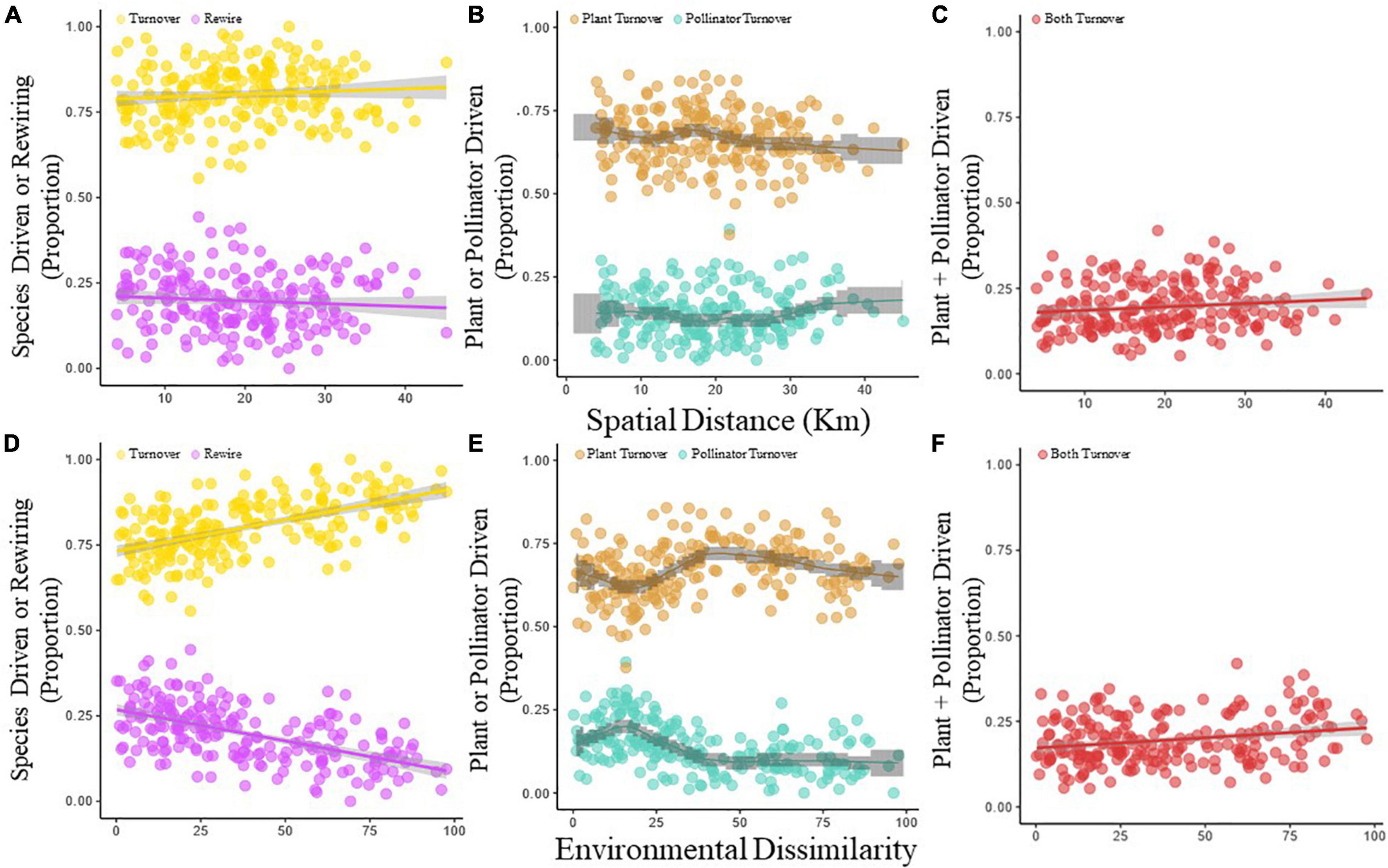
Figure 4. The proportion of the total interaction turnover that can be labeled as either species-driven interaction turnover (yellow points and yellow line) or rewiring (purple points and purple line) changes in relation to geographical distance (A) or the environmental dissimilarity (B) between paired networks. The proportion of the species–driven interaction turnover that can be ascribed as pollinator-driven (blue points and blue line) and plant-driven (orange points and orange line) as a function of spatial distance (C) or environmental dissimilarity (D). Proportion of species–driven interaction turnover that is caused by a combined turnover of both plants and pollinators (pollinator + plant-driven) in relation to geographical distance (E) and environmental dissimilarity (F).

The species driven turnover (I_species) was further partitioned into plant (T_pla), pollinator (T_pol) and plant + pollinator (T_pla+pol) driven turnover (Figures 4B,C,E,F). Along both the spatial and environmental dissimilarity gradient, plant driven interaction turnover contributed more to species driven interaction turnover than pollinator driven (T_pla > T_pol, Figures 4B,E), accounting for ∼70% of species driven interaction turnover. While spatial distance did not have much impact on proportional contributions (the bootstrap limits did not show a trend, Figure 4B; see Supplementary Table S7 for non-significant mantel test), the proportion of plant and pollinator turnover varied as a function of enviromental dissimilarity (Figure 4E). The effect was most pronounced at small environmental dissimilarities, where pollinator driven turnover peaked and plant driven turnover reached its minimum. For pollinator driven turnover, this was significant as the lower limits of the bootstrap confidence bands at environmental dissimilarity score of 15 were higher than the upper limits at other dissimilarities, while for plant driven turnover, the peak occurred at a score of 45, where the lower confidence band is higher than the upper limits at other landscape dissimilarities.

The plant and pollinator driven turnover (T_pol+pla) contributed 15% to all interaction turnover (Figure 4C), meaning in any given network comparision, 15% of interactions will be between plant and pollinator species unique to either network. Spatial distance had a non-significant postive effect on the contribution of unique interaction to interaction turnover (Mantel test with 999 permutations: r_M = 0.1274, p = 0.103; Figure 4C), while the unique interaction contribution to interaction turnover increased linearly with gradient dissimilarity (Mantel test with 999 permutations: r_M = 0.2256, p = 0.027; Figure 4F).

Predicting Interaction Turnover

The prediction performance of the mixed effects model and the random effects model was similar for each component of interaction turnover, indicating that the fixed effects added little useful information for predicting interaction turnover (see AUC values in Supplementary Table S18 and Figure 5). The good predictive performance of the random effects models indicates that most of the variation in whether an interaction will turnover or not is contained in the species under comparison. The prediction performance of the GLM was poor for pollinator driven turnover (AUC = 0.62), plant driven turnover (AUC = 0.65) and plant and pollinator driven turnover (AUC = 0.58), yet performed reasonably well for rewiring (AUC = 0.87, Supplementary Table S18), meaning that the fixed effects, composed of landscape variables (gradient dissimilarity, average impervious index and average agricultural intensity index, spatial distance), interaction properties (average interaction frequency) and ecological variables (plant origin and difference in floral abundance) can be used to predict interaction rewiring (Figure 5). Yet, this predictive performance is lower compared to the random effects model (random effects model AUC = 0.93), meaning that much of the variance in whether an interaction would rewire is dependent on the species in question and less so on the surrounding environment. For pollinator driven, plant driven and plant and pollinator driven interaction turnover the GLMs performed very poorly in comparison to the random effects GLMMs (see Figure 5 or Supplementary Table S18 for comparison of AUC values), illustrating that whether an interaction turned over due to species driven turnover is dependent on the species in question and not on the measured site variables or interaction properties. See Supplementary Material Prediction of Interaction Turnover for full discussion of results, particularly Supplementary Table S18.

FIGURE 5

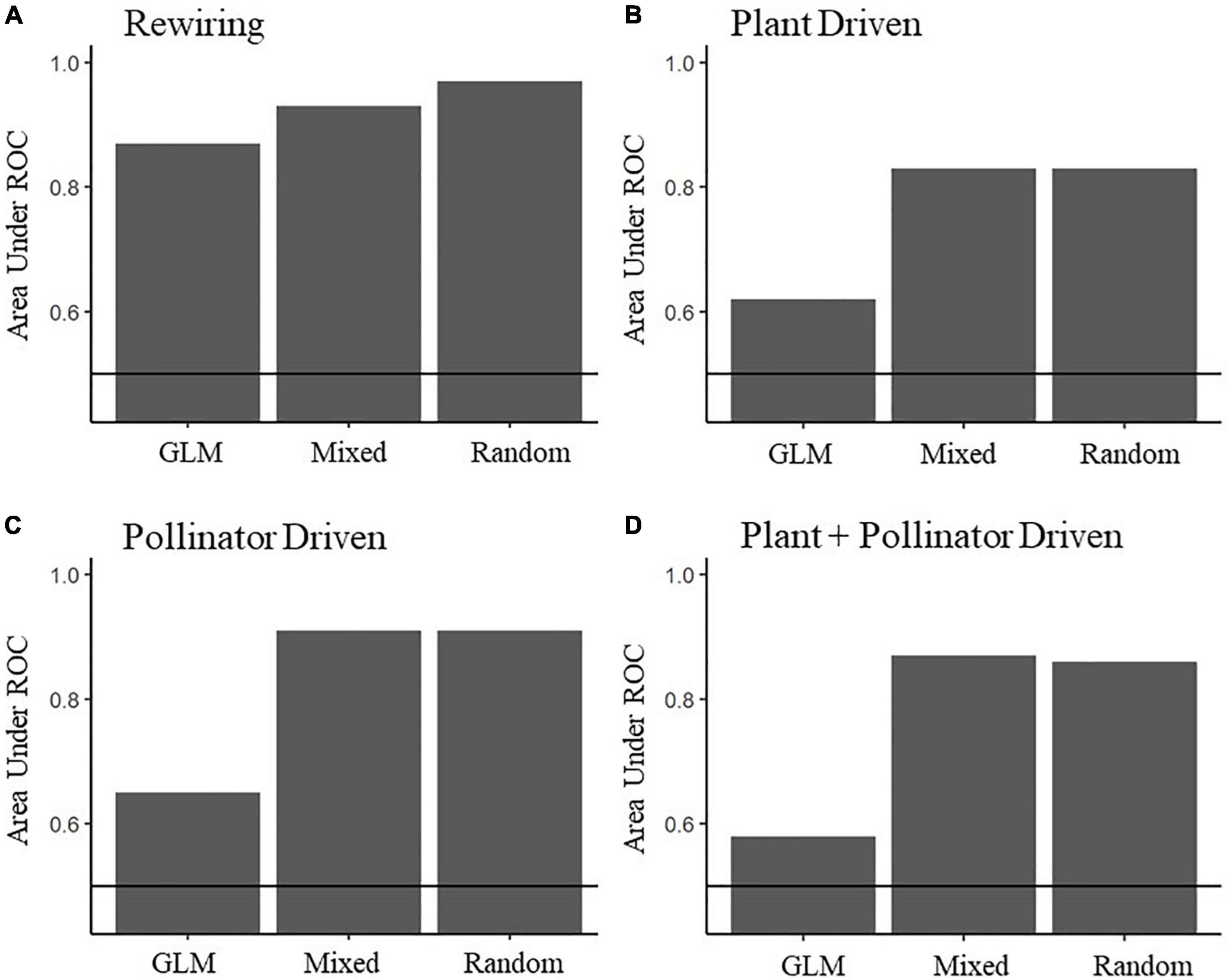
Figure 5. Area under the Receiver Operating Curve (AUC) values for models predicting interaction rewiring (A), plant driven interaction turnover (B), pollinator driven interaction turnover (C), and both plant + pollinator driven interaction turnover (D). The receiver operating curve is created by plotting the true positive rate (TPR) against the false positive rate (FPR) at various threshold settings. The closer AUC is to one, the better the model performance. GLM refers to a model using landscape, ecological and network variables, Mixed refers to a GLMM with landscape, ecological and network variables as fixed effects and species identity as random effects and Random refers to a GLMM using species identity as random effects. The horizontal line is 0.5 AUC, where the model performs no better than random.

The binomial GLM for rewiring performed reasonably well (AUC = 0.87) indicating that the covariates are useful for predicting when an interaction will rewire or stay constant. Average interaction frequency correlated negatively with interaction turnover, meaning interactions that were frequent rewired less (Figure 6A), while the average agricultural index, the average impervious index and the environmental dissimilarity (Figures 6B–D) were positively correlated with interaction turnover, meaning that interaction pairs in differing landscape intensities and types were more likely to rewire. Plant origin, whether native or introduced, affected the probability of interaction turnover, with native plants having a lower mean turnover probability (Figure 6E). Finally, a lot of variation is contained at the species level, with the impact of average interaction frequency conditioned strongly be species identity (Figure 6F). See Supplementary Table S10 for model outputs and summaries of the binomial GLM.

FIGURE 6

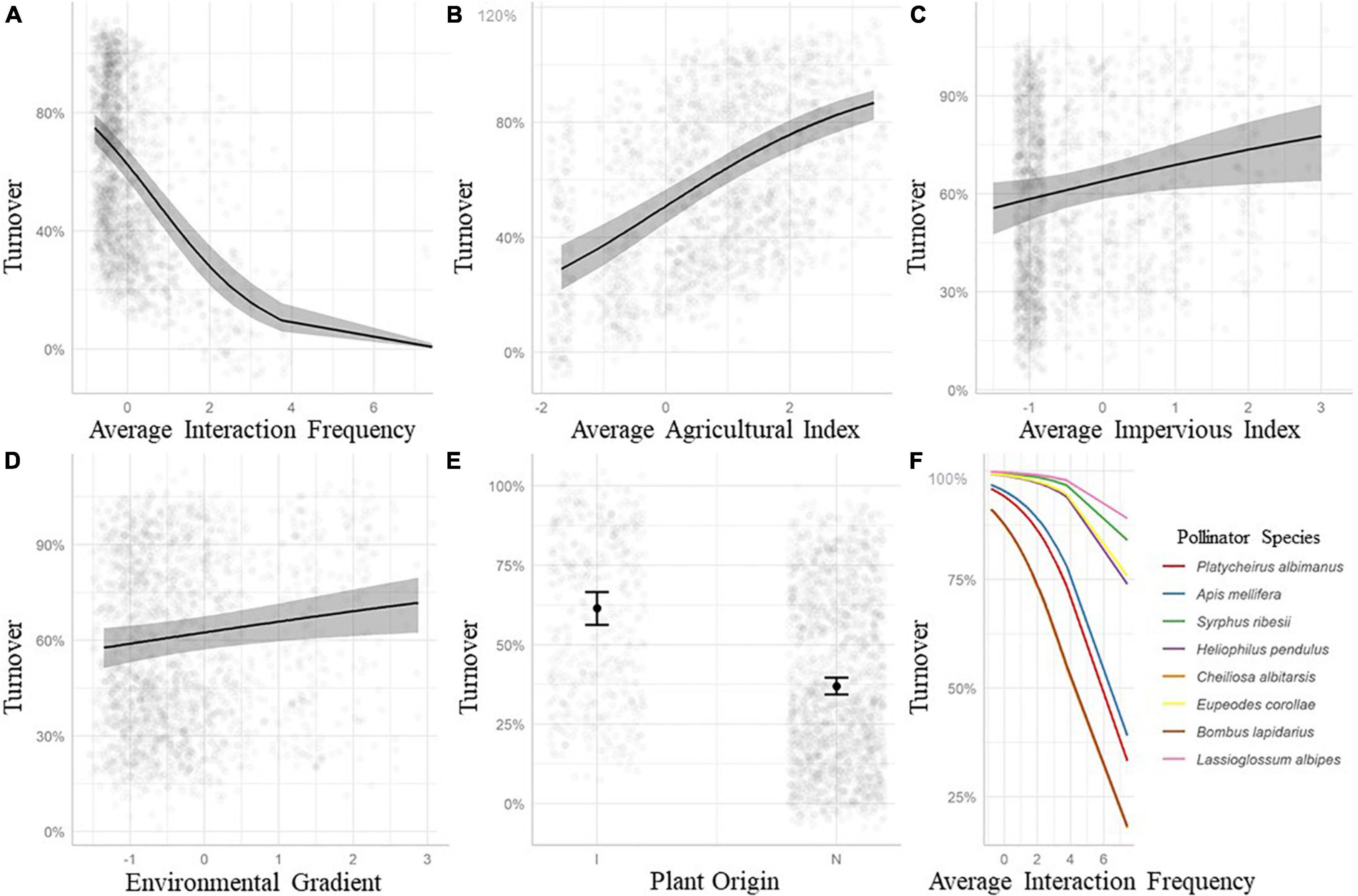
Figure 6. Probability of interaction turnover and model predictors based on a binomial GLM predicting rewiring (A–E) and a sample of individual pollinator responses from a binomial GLMM (F). (A) Average interaction frequency is negatively related to the probability of interaction turnover. The more frequent interactions show lower probabilities of turnover between sites. (B) The larger the average agricultural index of the site pair, the higher the probability that an interaction turns over. (C) The larger the average impervious index of the site pair, the higher the probability that an interaction turns over. (D) The more dissimilar the environmental gradient is between site pairs, the higher the probability that an interaction turns over. (E) Probability of interaction turnover for native and introduced plant species. (F) Large variance in how the interaction turnover of individual pollinator species changes with average interaction frequency. Superimposed residuals result in darker marks (A–E). See Supplementary Table S10 for binomial GLM parameter estimates and Supplementary Table S9 for mixed effects GLMM parameter estimates and random effect variances.

Discussion

Community Dissimilarity

The beta diversity of interaction networks is structured strongly by anthropogenic landscapes, and to a lesser extent by geographical proximity (Figure 3). The mechanism structuring the interaction networks is likely anthropogenic environmental filtering of the plant community, as the plant beta diversity patterns are strongly structured by the anthropogenic landscapes, while pollinator beta diversity is not. Additionally, plant driven interaction turnover is the dominant component of interaction turnover (Figure 4) and so drives the observed patterns in network beta diversity. Previous studies have shown distance decay effects for plant-pollinator interaction networks across a variety of spatial scales (Carstensen et al., 2014; Trøjelsgaard et al., 2015), yet to our knowledge, this is the first evidence that environmental gradients (in this case, urbanization and agricultural intensification) structure interaction beta diversity, and indeed can exert a greater structuring force than spatial distance.

Network beta diversity patterns show a degree of spatial structure, some of which can be accounted for by the spatial structure present in the pollinator community (Figure 3). Yet, the variation partitioning procedure estimated the independent spatial component to account for 8% of the network beta diversity variation (Supplementary Figure S11F), demonstrating that interactions are subject to spatial processes that do not operate for their constituent organisms. Similarly, a further 8% of variation is partitioned into the purely environmental component, providing evidence that interactions have their own biogeographic patterns not determined exclusively by their respective communities. Using a different method, Poisot et al. (2012) found a similar pattern, the dissimilarity of interactions formed by species shared between sites shows no correlation with the dissimilarity of species composition, implying that environmental filtering of species and interactions are different. Thus, if we are to build a predictive biogeography of ecological interactions, we are not only required to model species co-occurrence as influenced by environmental and spatial data but also must model the influence of such variables on the likelihood of interactions occurring. We must condition interaction probabilities on the environment and spatial distance (Gravel et al., 2019).

Networks and plant communities that occur in sites with similar environmental characteristics were more similar than expected by the null model distribution (Figure 3). This is likely an effect of local environmental filtering, where plant species and thus interactions in similar landscapes were selected for. The native plant community is responsible for this pattern, as opposed to the non-native plant community (Supplementary Figure S9), and so we can rule out the effect of human preferences for garden and agricultural plant species in generating more similar than expected communities. This suggests that the environmental context, the degree of urbanization or intensity of agriculture, is strongly filtering native plant community composition, generating homogenous native plant communities in similar landscapes. Interestingly, there were only three plant communities that were more dissimilar than expected by the null model distribution (Figure 3), meaning that both the spatial distance and environmental dissimilarity between sites were not great enough to create plant communities and networks significantly different in their composition. Studies have found that networks that are far apart (∼450 km) are more different than expected under randomization (Trøjelsgaard et al., 2015), suggesting that the spatial distance of this study (50 km) was not large enough for dispersal limitation to have an effect. Yet, it is surprising that the relatively large differences in the anthropogenic gradient, comparing sites in an urban center to sites with a significant proportion of semi-natural habitat to sites in intensive agriculture, did not produce plant, pollinator communities or interaction networks that were significantly different from each other. Overall, that plant communities and networks are more similar than expected in similar landscapes is suggestive of homogenization within anthropogenic land use classes, a finding similar to studies that show intense agriculture erodes beta diversity (Karp et al., 2012) or that residential lawns homogenize urban plant communities (Wheeler et al., 2017). Yet, we do not find homogenization of communities along the urban and agricultural intensification gradients (Supplementary Figure S7), suggesting that the pattern observed here is not one of homogenization with intensity of land use, but rather of community homogenization within landscape types.

It should be noted that most of the variation in the plant and pollinator communities and in interaction networks could not be explained by either the measured environmental variables or spatial distance, indicating that while urbanization and agricultural intensification do structure communities and interaction networks, they account for a relatively small proportion of the total dissimilarity. Thus, while we conclude that landscape scale anthropogenic environmental filtering is contributing to structuring community assembly and interaction formation in our study region, the major structuring processes have not been elucidated. A potential reason for the low explanatory power is that local habitat filtering effects are unaccounted for in the analysis, as aggregating communities and networks collected in different habitats into a landscape level community or network obscures local habitat filtering.

Components of Interaction Turnover

As in other studies, species driven interaction turnover was the major component of interaction turnover, accounting for ∼80% of the turnover in interactions. Increasing spatial distance had no effect on the proportion of rewiring or species driven interaction turnover, in contrast to a previous study conducted a study at a larger spatial scale (Trøjelsgaard et al., 2015), again suggesting that geographical effects occur at larger spatial scales than the 50 km scale of the present study. However, increasing environmental dissimilarity had a strong effect, increasing the proportion of species driven turnover and decreasing the rewiring contribution. The contribution of rewiring more than halves across the anthropogenic dissimilarity gradient: rewiring contributes ∼25% at low anthropogenic dissimilarity but less than 10% at high anthropogenic dissimilarity. Importantly, the fact that rewiring contributes double digit proportions to interaction turnover means that any study that attempts to understand the impacts of environmental change on ecological networks must account for rewiring or risk underestimating the impact of environmental change.

Disaggregating species driven interaction turnover into its respective components reveals that plant species turnover accounts for 70% of all species driven interaction turnover. A previous study in a more natural area found that pollinator-drive interaction turnover was the major component (Trøjelsgaard et al., 2015). This suggests that in urban and agricultural environments, where the native plant species pool is supplemented with non-natives, plant driven turnover is the dominant component of network beta diversity.

Plants and pollinators appear to be affected differently by anthropogenic dissimilarity, with a peak for pollinator driven interaction turnover at low gradient dissimilarity while the peak for plant driven interaction turnover occurred at medium levels of gradient dissimilarity. This is consistent with the respective responses of the plant and pollinator communities to anthropogenic dissimilarity. Plant community dissimilarity is more strongly correlated to anthropogenic dissimilarity than the pollinator community is, and thus we should expect the proportion of plant driven interaction turnover to increase as anthropogenic dissimilarity increases. A weak positive effect of environmental dissimilarity on plant + pollinator driven interaction turnover existed, meaning a complete substitution of both plants and pollinators accounted for an increasing fraction of species driven turnover in landscapes with increasingly different compositions. In the Canary Islands, Trøjelsgaard et al. (2015) found that these entirely novel interactions dominate interaction turnover at regional spatial scales, yet in strongly contrasting anthropogenic landscapes complete substitution only accounts for ∼25% of interaction turnover. Thus, while the anthropogenic gradients likely impose habitat filtering effects resulting in complete substitution and novel interactions, the strength of the anthropogenic filtering effect is not as strong as island biogeographic dispersal limitation and habitat filtering.

We encourage replication of this study in other contexts, particularly along anthropogenic gradients. Ireland is known to have a depauperate pollinator community compared to the British Isles and particularly Mediterranean Europe, and the trends revealed here - turnover of the plant community is the dominant component of interaction turnover - may not be so dominant in regions with a richer pollinator fauna. Island biogeographic factors could play a role in which component is dominant as the study of Trøjelsgaard et al. (2015) on the Canary Islands found that the pollinator community was the main component of network dissimilarity. Thus, determining what conditions pollinator turnover vs. plant turnover is the dominant component of network dissimilarity is fruitful avenue of research.

Predicting Interaction Turnover

Pairwise interactions have proven difficult to predict (Burkle and Alarcón, 2011). Efforts in the last decade have moved toward probabilistic models that generate both interactions and networks, moving the field beyond descriptions of network structure (Strydom et al., 2021). Here, our aim was to explore which variables (species-level, environmental, spatial) influence the turnover of interactions to highlight the data required by probabilistic models to accurately predict patterns of network beta diversity.

We found that species driven interaction turnover, as opposed to rewiring, is difficult to predict without species level information. The site variables and interaction properties that we measured provided little useful information for predicting species driven interaction turnover. The inclusion of the species identities and the site pair combination as random effects drastically improved prediction performances, indicating that species specific variables are required to accurately predict species driven interaction turnover. As species driven turnover is the dominant component of interaction turnover in spatially separated networks, further work building probabilistic models to predict network beta diversity would benefit from adopting species distribution modeling practices, in particular joint species distribution models (Tikhonov et al., 2017) and interaction distribution modeling (Gravel et al., 2019). As the local species pool forms the basis of interaction networks, building probabilistic species pools based on spatially explicit distribution models is essential to predict networks across space (Strydom et al., 2021).

In contrast to species driven interaction turnover, it was possible to predict interaction rewiring to a reasonable degree of accuracy with site characteristics and interaction properties. Average interaction frequency was the most significant predictor of rewiring, with interactions that occurred frequently between co-occurring species much less likely to rewire. Interactions with high interaction frequency can be interpreted as linking species with high mutual affinity, it is likely that such species would interact with high frequency if no temporal or spatial constraints are imposed (Carstensen et al., 2014). These interactions were likely a result of both niche and neutral processes: at a minimum, these interactions were not forbidden due to trait mismatches and were likely heavily influenced by the relative abundances of the respective species (Poisot et al., 2014). Additionally, the relative difference in plant abundance between a site pair showed a positive relationship with rewiring, meaning that increasing the difference in plant floral abundance between a site pair increased the likelihood of interaction turnover, underscoring how important neutral processes are to interaction formation. Yet, interaction frequency in pollination systems is difficult to predict (Strydom et al., 2021) and, to the best of our knowledge, models predicting floral abundance for each species within a community do not exist. Thus, the more useful variables for predicting rewiring are currently unavailable to probabilistic network modelers interested in exploring network dissimilarity across space and time. The long-standing assumption that co-occurrence is equivalent to meaningful interaction strength has been shown to be false (Blanchet et al., 2020), and thus to predict rewiring, a significant component of network dissimilarity accounting for ∼20% of interaction turnover in our study, species level information on abundance and traits are particularly important in constraining the set of possible networks generated from probabilistic models. The proliferation of open access databases, such as those on plant functional traits (TRY⁷), species interaction data (Mangal⁸ and GloBI⁹) and metacommunity ecology and species trait data¹⁰ could facilitate the development of predictive models of interaction strength and floral abundance.

Landscape level variables were predictive of rewiring, particularly agricultural intensity which increased the likelihood of rewiring strongly. Interestingly, this would increase the beta diversity of interaction networks in intensive agricultural landscapes, contrasting with the homogenization of the plant communities in such landscapes (Karp et al., 2012). A much weaker positive effect of the impervious gradient was found, indicating that urbanization also increases the probability of interaction rewiring. However, the urbanization effect was not retained in the mixed effects model, and so we can conclude that while agricultural intensification shows a strong and consistent effect of increased rewiring probability, the evidence for urbanization is mixed and needs further exploration. Additionally, the gradient dissimilarity between site pairs increased the probability of an interaction rewiring, indicating an effect of landscape composition. That these landscape variables impact rewiring probabilities highlights that remote sensing can be a useful data source for models seeking to enhance predictive power. Yet, the random effects GLMM still outperformed the binomial GLM to such a degree that if we are to build predictive models of interaction rewiring, and more generally of interaction turnover, it would be more fruitful to build predictive models using species level information. Gravel et al. (2019) proposes to build probabilistic models of species interactions which combines species distribution modeling and species level trait data to model the probability of interactions between species. The probabilistic approach is data intensive, yet this study has shown that to accurately predict interaction turnover, species level data are required.

Conclusion

Using methods and tools developed to make interaction networks amenable to community ecology analysis, we have shown that an anthropogenic environmental gradient structures the composition of interaction networks while geographical distance exerts a weaker effect, to our knowledge the first study to do so. A similar pattern is observed with the components of interaction turnover, demonstrating that the anthropogenic gradient moderates the components of interaction turnover and not geographical distance, highlighting the importance of considering anthropogenic disturbances in studying the biogeography of interaction networks. Yet, when it comes to predicting when an interaction turns over, site characteristics and interaction properties perform poorly, showing that if we are to build a more predictive science of the biogeography of interaction networks, there is still much work to be done to integrate species specific responses. Given that species driven interaction turnover is the main component of the patterns observed in this study, extending species distribution modeling to interaction distribution modeling is a promising avenue of further research.

Data Availability Statement

The datasets presented in this study can be found in online repositories. The names of the repository/repositories and accession number(s) can be found below: for R scripts, data analysis workflow and data see my GitHub: https://github.com/ciwhite/network_beta_diversity; for the data see FigShare: https://figshare.com/articles/dataset/Beta_Diversity_of_Plant-Pollinator_Interactions_in_Anthropogenic_Landscapes/16910902.

Author Contributions

CW and JS conceived of the study design. CW carried out data collection and analysis. CW was carried out the writing with commenting and editing from JS and MC. All authors contributed to the article and approved the submitted version.

Funding

The research leading to this manuscript has received funding from the European Community’s Framework Program Horizon 2020 for the Connecting Nature Project (Grant Agreement number: 730222) and from the Trinity College Dublin studentship.

Conflict of Interest

The authors declare that the research was conducted in the absence of any commercial or financial relationships that could be construed as a potential conflict of interest.

Publisher’s Note

All claims expressed in this article are solely those of the authors and do not necessarily represent those of their affiliated organizations, or those of the publisher, the editors and the reviewers. Any product that may be evaluated in this article, or claim that may be made by its manufacturer, is not guaranteed or endorsed by the publisher.

Acknowledgments

Tom Gittings for verifying hoverfly identifications and to Una Fitzpatrick and Tomas Murray of the National Biodiversity Data Centre for assistance in verifying the bees. Laura Russo for introducing the process of taxonomic identification of insects and for lots of very helpful assistance and advice. All R code and custom functions are available at: https://github.com/ciwhite/network_beta_diversity. All data (interaction network data, environmental conditions and site coordinates) are made available on at: https://figshare.com/projects/Network_Beta_Diversity/134342.

Supplementary Material

The Supplementary Material for this article can be found online at: https://www.frontiersin.org/articles/10.3389/fevo.2022.806615/full#supplementary-material

Footnotes

1. ^ https://identify.plantnet.org/
2. ^ https://www.google.com/maps/d/
3. ^ https://land.copernicus.eu/local/urban-atlas
4. ^ https://land.copernicus.eu/local/urban-atlas/urban-atlas-2012
5. ^ https://www.npws.ie/maps-and-data/habitat-and-species-data
6. ^ https://identify.plantnet-project.org/
7. ^ https://www.try-db.org/TryWeb/About.php
8. ^ https://mangal.io/#/
9. ^ https://www.globalbioticinteractions.org/about
10. ^ https://icestes.github.io/

References

Alberti, M. (2010). Maintaining ecological integrity and sustaining ecosystem function in urban areas. Curr. Opin. Environ. Sustainabil. 2, 178–184.

Google Scholar

Alberti, M., Correa, C., Marzluff, J. M., Hendry, A. P., Palkovacs, E. P., Gotanda, K. M., et al. (2017a). Global urban signatures of phenotypic change in animal and plant populations. Proc. Natl. Acad. Sci. U S A. 114, 8951–8956. doi: 10.1073/pnas.1606034114

PubMed Abstract | CrossRef Full Text | Google Scholar

Alberti, M., Marzluff, J., and Hunt, V. M. (2017b). Urban driven phenotypic changes: empirical observations and theoretical implications for eco-evolutionary feedback. Philos. Trans. R. Soc. B: Biol. Sci. 372:20160029. doi: 10.1098/rstb.2016.0029

PubMed Abstract | CrossRef Full Text | Google Scholar

Anderson, M. J., Crist, T. O., Chase, J. M., Vellend, M., Inouye, B. D., Freestone, A. L., et al. (2011). Navigating the multiple meanings of β diversity: a roadmap for the practicing ecologist. Ecol. Lett. 14, 19–28. doi: 10.1111/j.1461-0248.2010.01552.x

PubMed Abstract | CrossRef Full Text | Google Scholar

Baldock, K. C., Goddard, M. A., Hicks, D. M., Kunin, W. E., Mitschunas, N., Osgathorpe, L. M., et al. (2015). Where is the UK’s pollinator biodiversity? the importance of urban areas for flower-visiting insects. Proc. R. Soc. B: Biol. Sci. 282:20142849. doi: 10.1098/rspb.2014.2849

PubMed Abstract | CrossRef Full Text | Google Scholar

Banaszak-Cibicka, W., and Żmihorski, M. (2012). Wild bees along an urban gradient: winners and losers. J. Insect Conserv. 16, 331–343.

Google Scholar

Bascompte, J., and Jordano, P. (2013). Mutualistic Networks. Princeton, NJ: Princeton University Press.

Google Scholar

Bates, A. J., Sadler, J. P., Fairbrass, A. J., Falk, S. J., Hale, J. D., and Matthews, T. J. (2011). Changing bee and hoverfly pollinator assemblages along an urban-rural gradient. PLoS One 6:e23459. doi: 10.1371/journal.pone.0023459

PubMed Abstract | CrossRef Full Text | Google Scholar

Bates, D., Maechler, M., Bolker, B., and Walker, S. (2015). Fitting linear mixed-effects models using lme4. J. Statistical Software 67, 1–48. doi: 10.18637/jss.v067.i01

CrossRef Full Text | Google Scholar

Beckmann, M., Gerstner, K., Akin-Fajiye, M., Ceau?u, S., Kambach, S., Kinlock, N. L., et al. (2019). Conventional land-use intensification reduces species richness and increases production: a global meta-analysis. Global Change Biol. 25, 1941–1956. doi: 10.1111/gcb.14606

PubMed Abstract | CrossRef Full Text | Google Scholar

Blair, R. B. (1999). Birds and butterflies along an urban gradient: surrogate taxa for assessing biodiversity? Ecol. Appl. 9, 164–170.

Google Scholar

Blanchet, F. G., Cazelles, K., and Gravel, D. (2020). Co-occurrence is not evidence of ecological interactions. Ecol. Lett. 23, 1050–1063. doi: 10.1111/ele.13525

PubMed Abstract | CrossRef Full Text | Google Scholar

Burkle, L. A., and Alarcón, R. (2011). The future of plant–pollinator diversity: understanding interaction networks across time, space, and global change. Am. J. Botany 98, 528–538. doi: 10.3732/ajb.1000391

PubMed Abstract | CrossRef Full Text | Google Scholar

Burkle, L. A., Myers, J. A., and Belote, R. T. (2016). The beta-diversity of species interactions: untangling the drivers of geographic variation in plant–pollinator diversity and function across scales. Am. J. Botany 103, 118–128. doi: 10.3732/ajb.1500079

PubMed Abstract | CrossRef Full Text | Google Scholar

Cane, J. H., Minckley, R. L., Kervin, L. J., Roulston, T. A. H., and Williams, N. M. (2006). Complex responses within a desert bee guild (Hymenoptera: Apiformes) to urban habitat fragmentation. Ecol. Appl. 16, 632–644. doi: 10.1890/1051-0761(2006)016[0632:crwadb]2.0.co;2

PubMed Abstract | CrossRef Full Text | Google Scholar

Carrier, J. A., and Beebee, T. J. (2003). Recent, substantial, and unexplained declines of the common toad Bufo bufo in lowland England. Biol. Conserv. 111, 395–399.

Google Scholar

Carstensen, D. W., Sabatino, M., Trøjelsgaard, K., and Morellato, L. P. C. (2014). Beta diversity of plant-pollinator networks and the spatial turnover of pairwise interactions. PLoS One 9:e112903. doi: 10.1371/journal.pone.0112903

PubMed Abstract | CrossRef Full Text | Google Scholar

Chase, J. M., Kraft, N. J., Smith, K. G., Vellend, M., and Inouye, B. D. (2011). Using null models to disentangle variation in community dissimilarity from variation in α-diversity. Ecosphere 2, 1–11.

Google Scholar

Dray, S., Matias, C., Miele, V., Ohlmann, M., and Thuiller, W. (2020a). econetwork: Analyzing Ecological Networks. R Package Version 0.4.1. Available online at: https://CRAN.R-project.org/package=econetwork.

Google Scholar

Dray, S., Bauman, D., Blanchet, G., Borcard, D., Clappe, S., Guenard, G., et al. (2020b). Adespatial: Multivariate Multiscale Spatial Analysis. R Package Version 0.3-8. Available online at: https://CRAN.R-project.org/package=adespatial.

Google Scholar

Dunne, J. A. (2006). The Network Structure of Food Webs. Oxford: Oxford University Press, 27–86.

Google Scholar

Ekroos, J., Heliölä, J., and Kuussaari, M. (2010). Homogenization of lepidopteran communities in intensively cultivated agricultural landscapes. J. Appl. Ecol. 47, 459–467.

Google Scholar

Elmqvist, T., Setälä, H., Handel, S. N., Van Der Ploeg, S., Aronson, J., Blignaut, J. N., et al. (2015). Benefits of restoring ecosystem services in urban areas. Curr. Opin. Environ. Sustainabil. 14, 101–108.

Google Scholar

Falk, S. J. (2015). Field Guide to the Bees of Great Britain and Ireland. Totnes: British Wildlife Publishing.

Google Scholar

Flohre, A., Fischer, C., Aavik, T., Bengtsson, J., Berendse, F., Bommarco, R., et al. (2011). Agricultural intensification and biodiversity partitioning in European landscapes comparing plants, carabids, and birds. Ecol. Appl. 21, 1772–1781. doi: 10.1890/10-0645.1

PubMed Abstract | CrossRef Full Text | Google Scholar

Foley, J. A., DeFries, R., Asner, G. P., Barford, C., Bonan, G., Carpenter, S. R., et al. (2005). Global consequences of land use. Science 309, 570–574.

Google Scholar

Fortel, L., Henry, M., Guilbaud, L., Guirao, A. L., Kuhlmann, M., Mouret, H., et al. (2014). Decreasing abundance, increasing diversity and changing structure of the wild bee community (Hymenoptera: Anthophila) along an urbanization gradient. PLoS One 9:e104679. doi: 10.1371/journal.pone.0104679

PubMed Abstract | CrossRef Full Text | Google Scholar

Fründ, J. (2021). Dissimilarity of species interaction networks: how to partition rewiring and species turnover components. Ecosphere. 12:e03653. doi: 10.1002/ecs2.3653

CrossRef Full Text | Google Scholar

Germaine, S. S., and Wakeling, B. F. (2001). Lizard species distributions and habitat occupation along an urban gradient in Tucson. Arizona, USA. Biol. Conserv. 97, 229–237.

Google Scholar

Gerstner, K., Dormann, C. F., Stein, A., Manceur, A. M., and Seppelt, R. (2014). EDITOR’S CHOICE: review: effects of land use on plant diversity–a global meta-analysis. J. Appl. Ecol. 51, 1690–1700.

Google Scholar

Geslin, B., Gauzens, B., Thebault, E., and Dajoz, I. (2013). Plant pollinator networks along a gradient of urbanisation. PLoS One 8:e63421. doi: 10.1371/journal.pone.0063421

PubMed Abstract | CrossRef Full Text | Google Scholar

Goddard, M. A., Dougill, A. J., and Benton, T. G. (2010). Scaling up from gardens: biodiversity conservation in urban environments. Trends Ecol. Evol. 25, 90–98. doi: 10.1016/j.tree.2009.07.016

PubMed Abstract | CrossRef Full Text | Google Scholar

Gravel, D., Baiser, B., Dunne, J. A., Kopelke, J. P., Martinez, N. D., Nyman, T., et al. (2019). Bringing Elton and Grinnell together: a quantitative framework to represent the biogeography of ecological interaction networks. Ecography 42, 401–415.

Google Scholar

Grimm, N. B., Faeth, S. H., Golubiewski, N. E., Redman, C. L., Wu, J., Bai, X., et al. (2008). Global change and the ecology of cities. Science 319, 756–760. doi: 10.1126/science.1150195

PubMed Abstract | CrossRef Full Text | Google Scholar

Hall, D. M., Camilo, G. R., Tonietto, R. K., Ollerton, J., Ahrné, K., Arduser, M., et al. (2017). The city as a refuge for insect pollinators. Conserv. Biol. 31, 24–29. doi: 10.1111/cobi.12840

PubMed Abstract | CrossRef Full Text | Google Scholar

Hanley, J. A., and McNeil, B. J. (1982). The meaning and use of the area under a receiver operating characteristic (ROC) curve. Radiology 143, 29–36. doi: 10.1148/radiology.143.1.7063747

PubMed Abstract | CrossRef Full Text | Google Scholar

Harrison, T., and Winfree, R. (2015). Urban drivers of plant-pollinator interactions. Funct. Ecol. 29, 879–888.

Google Scholar

Hartig, F. (2020). DHARMa: Residual Diagnostics for Hierarchical (Multi-Level/Mixed) Regression Models. R Package Version 0.3.3.0. Available online at: https://CRAN.R-project.org/package=DHARMa.

Google Scholar

Hawkins, C. P., Mykrä, H., Oksanen, J., and Vander Laan, J. J. (2015). Environmental disturbance can increase beta diversity of stream macroinvertebrate assemblages. Global Ecol. Biogeography 24, 483–494. doi: 10.1111/gcb.15389

PubMed Abstract | CrossRef Full Text | Google Scholar

IPBES (2018). “The IPBES assessment report on land degradation and restoration,” in Secretariat of the Intergovernmental Science-Policy Platform on Biodiversity and Ecosystem Services, eds L. Montanarella, R. Scholes, and A. Brainich (Germany: Bonn).

Google Scholar

Karp, D. S., Rominger, A. J., Zook, J., Ranganathan, J., Ehrlich, P. R., and Daily, G. C. (2012). Intensive agriculture erodes β-diversity at large scales. Ecol. Lett. 15, 963–970. doi: 10.1111/j.1461-0248.2012.01815.x

PubMed Abstract | CrossRef Full Text | Google Scholar

Keddy, P. A. (1992). Assembly and response rules: two goals for predictive community ecology. J. Vegetation Sci. 3, 157–164.

Google Scholar

Kremen, C., Williams, N. M., and Thorp, R. W. (2002). Crop pollination from native bees at risk from agricultural intensification. Proc. Natl. Acad. Sci. U S A. 99, 16812–16816. doi: 10.1073/pnas.262413599

PubMed Abstract | CrossRef Full Text | Google Scholar

Le Féon, V., Schermann-Legionnet, A., Delettre, Y., Aviron, S., Billeter, R., Bugter, R., et al. (2010). Intensification of agriculture, landscape composition and wild bee communities: a large scale study in four European countries. Agriculture Ecosystems Environ. 137, 143–150.

Google Scholar

Li (2018). hillR: taxonomic, functional, and phylogenetic diversity and similarity through Hill Numbers. J. Open Source Software 3:1041. doi: 10.21105/joss.01041

CrossRef Full Text | Google Scholar

McKinney, M. L. (2002). Urbanization. Biodiversity Conserv. Biosci. 52, 883–890.

Google Scholar

McKinney, M. L. (2006). Urbanization as a major cause of biotic homogenization. Biol. Conserv. 127, 247–260.

Google Scholar

McKinney, M. L. (2008). Effects of urbanization on species richness: a review of plants and animals. Urban Ecosystems 11, 161–176. doi: 10.1016/j.envint.2015.09.013

PubMed Abstract | CrossRef Full Text | Google Scholar

McPhearson, T., Pickett, S. T., Grimm, N. B., Niemelä, J., Alberti, M., Elmqvist, T., et al. (2016). Advancing urban ecology toward a science of cities. BioScience 66, 198–212.

Google Scholar

Menke, S. B., Guénard, B., Sexton, J. O., Weiser, M. D., Dunn, R. R., and Silverman, J. (2011). Urban areas may serve as habitat and corridors for dry-adapted, heat tolerant species; an example from ants. Urban Ecosystems 14, 135–163.

Google Scholar

Nekola, J. C., and White, P. S. (1999). The distance decay of similarity in biogeography and ecology. J. Biogeography 26, 867–878.

Google Scholar

Newbold, T., Hudson, L. N., Hill, S. L., Contu, S., Lysenko, I., Senior, R. A., et al. (2015). Global effects of land use on local terrestrial biodiversity. Nature 520, 45–50. doi: 10.1038/nature14324

PubMed Abstract | CrossRef Full Text | Google Scholar

Novotny, V. (2009). Beta diversity of plant–insect food webs in tropical forests: a conceptual framework. Insect Conservation Diversity 2, 5–9.

Google Scholar

Ohlmann, M., Miele, V., Dray, S., Chalmandrier, L., O’connor, L., and Thuiller, W. (2019). Diversity indices for ecological networks: a unifying framework using Hill numbers. Ecol. Lett. 22, 737–747. doi: 10.1111/ele.13221

PubMed Abstract | CrossRef Full Text | Google Scholar

Oksanen, J., Blanchet, G. F., Friendly, M., Kindt, R., Legendre, P., McGlinn, D., et al. (2019). vegan: Community Ecology Package. R package Version 2.5-6. Available online at: https://CRAN.R-project.org/package=vegan.

Google Scholar

Pellissier, L., Albouy, C., Bascompte, J., Farwig, N., Graham, C., Loreau, M., et al. (2018). Comparing species interaction networks along environmental gradients. Biol. Rev. 93, 785–800. doi: 10.1111/brv.12366

PubMed Abstract | CrossRef Full Text | Google Scholar

Poisot, T., Canard, E., Mouillot, D., Mouquet, N., and Gravel, D. (2012). The dissimilarity of species interaction networks. Ecol. Lett. 15, 1353–1361. doi: 10.1111/ele.12002

PubMed Abstract | CrossRef Full Text | Google Scholar

Poisot, T., Stouffer, D. B., and Gravel, D. (2014). Beyond species: why ecological interaction networks vary through space and time. Oikos 124, 243–251.

Google Scholar

Potts, S. G., Biesmeijer, J. C., Kremen, C., Neumann, P., Schweiger, O., and Kunin, W. E. (2010). Global pollinator declines: trends, impacts and drivers. Trends Ecol. Evol. 25, 345–353. doi: 10.1016/j.tree.2010.01.007

PubMed Abstract | CrossRef Full Text | Google Scholar

R Core Team (2020). R: A Language and Environment for Statistical Computing. Vienna: R Foundation for Statistical Computing.

Google Scholar

Rader, R., Bartomeus, I., Tylianakis, J. M., and Laliberté, E. (2014). The winners and losers of land use intensification: pollinator community disassembly is non-random and alters functional diversity. Diversity Distribut. 20, 908–917.

Google Scholar

Ricketts, T. H., Regetz, J., Steffan-Dewenter, I., Cunningham, S. A., Kremen, C., Bogdanski, A., et al. (2008). Landscape effects on crop pollination services: are there general patterns? Ecol. Lett. 11, 499–515. doi: 10.1111/j.1461-0248.2008.01157.x

PubMed Abstract | CrossRef Full Text | Google Scholar

Rose, F., and O’Reilly, C. (2006). The Wild Flower Key (Revised Edition)-How to Identify Wild Plants, Trees and Shrubs in Britain and Ireland. London: Warne & Co.

Google Scholar

Santangelo, J. S., Rivkin, L. R., and Johnson, M. T. (2018). The evolution of city life. Proc. R. Soc. B 285:20181529.

Google Scholar

Seto, K. C., Sánchez-Rodríguez, R., and Fragkias, M. (2010). The new geography of contemporary urbanization and the environment. Ann. Rev. Environ. Resources 35, 167–194.

Google Scholar

Shochat, E., Lerman, S. B., Anderies, J. M., Warren, P. S., Faeth, S. H., and Nilon, C. H. (2010). Invasion, competition, and biodiversity loss in urban ecosystems. BioScience 60, 199–208. doi: 10.1007/s00442-020-04603-1

PubMed Abstract | CrossRef Full Text | Google Scholar

Shochat, E., Warren, P. S., Faeth, S. H., McIntyre, N. E., and Hope, D. (2006). From patterns to emerging processes in mechanistic urban ecology. Trends Ecol. Evol. 21, 186–191. doi: 10.1016/j.tree.2005.11.019

PubMed Abstract | CrossRef Full Text | Google Scholar

Simanonok, M. P., and Burkle, L. A. (2014). Partitioning interaction turnover among alpine pollination networks: spatial, temporal, and environmental patterns. Ecosphere 5, 1–17.

Google Scholar

Strydom, T., Catchen, M. D., Banville, F., Caron, D., Dansereau, G., Desjardins-Proulx, P., et al. (2021). A roadmap towards predicting species interaction networks (across space and time). Philos. Trans. R. Soc. B 376:20210063. doi: 10.1098/rstb.2021.0063

PubMed Abstract | CrossRef Full Text | Google Scholar

Stubbs, A. E., and Falk, S. J. (2002). British Hoverflies: An Illustrated Identification Guide. Wokingham: British Entomological and Natural History Society.

Google Scholar

Theodorou, P., Albig, K., Radzevičiūtė, R., Settele, J., Schweiger, O., Murray, T. E., et al. (2017). The structure of flower visitor networks in relation to pollination across an agricultural to urban gradient. Funct. Ecol. 31, 838–847.

Google Scholar

Tikhonov, G., Abrego, N., Dunson, D., and Ovaskainen, O. (2017). Using joint species distribution models for evaluating how species-to-species associations depend on the environmental context. Methods Ecol. Evol. 8, 443–452.

Google Scholar

Trøjelsgaard, K., Jordano, P., Carstensen, D. W., and Olesen, J. M. (2015). Geographical variation in mutualistic networks: similarity, turnover and partner fidelity. Proc. R. Soc. B: Biol. Sci. 282:20142925. doi: 10.1098/rspb.2014.2925

PubMed Abstract | CrossRef Full Text | Google Scholar

Vellend, M., Verheyen, K., Flinn, K. M., Jacquemyn, H., Kolb, A., Van Calster, H., et al. (2007). Homogenization of forest plant communities and weakening of species–environment relationships via agricultural land use. J. Ecol. 95, 565–573.

Google Scholar

Wehrens, R., Putter, H., and Buydens, L. M. (2000). The bootstrap: a tutorial. Chemometrics Intell. Lab. Systems 54, 35–52.

Google Scholar

Wheeler, M. M., Neill, C., Groffman, P. M., Avolio, M., Bettez, N., Cavender-Bares, J., et al. (2017). Continental-scale homogenization of residential lawn plant communities. Landscape Urban Plann. 165, 54–63. doi: 10.1002/eap.2455

PubMed Abstract | CrossRef Full Text | Google Scholar