Abstract
The rapid urbanization in China urges scholars to investigate the impacts of built environment on the level of travel satisfaction of rural residents to improve their quality of life and make planning exercises more human-centric. This study samples six villages out of the 25 top rural areas in Chengdu, Sichuan, China, as the research object and constructs a structural equation model to explore the direct and indirect impacts of the built environment on daily travel satisfaction of rural residents. The research finds that building density (0.609), road density (0.569), the number of accessible markets (0.314), and private car ownership (0.02) have significant positive impacts on travel satisfaction. Public transport (−0.063) has a direct negative impact on travel satisfaction. Consequently, in order to further improve travel satisfaction, construction departments and rural planners should improve the building and road densities of new rural areas and increase the number of accessible markets. The convenience of rural public transport services also needs improvement.
Introduction
Travel is an essential activity in people’s daily life (Yang et al., 2022). Travel satisfaction has been defined as people’s comprehensive evaluation and subjective feeling of transportation facilities and services (Gao et al., 2017a,b). Travel satisfaction reflects the quality of transportation services and can guide planners in providing good travel services for improving public health through transportation (Zhu and Fan, 2018a).
Research on travel satisfaction began in the 1960s and has been an area of research since (Diana, 2011; Abenoza et al., 2017; Gao et al., 2017b; Susilo et al., 2017; Mouratidis et al., 2019; Wang et al., 2020). In the past studies, scholars usually considered the influence of local population characteristics and travel-related variables (e.g., travel mode and travel time) on travel satisfaction (Olsson et al., 2013; St-Louis et al., 2014; De Vos et al., 2016; Ye and Titheridge, 2017; Mouratidis et al., 2019) and confirmed that various factors had a significant impact on travel satisfaction. For example, residents living in the city have a higher level of travel satisfaction when using bicycles (Mouratidis et al., 2019). Travel satisfaction will be remarkably reduced as a result of increasing population and motor vehicles, and the consequent extension in commuting time will result in low satisfaction (Meng et al., 2013). In recent years, studies have gradually incorporated the built environment (Ye and Titheridge, 2017; Zhao and Li, 2018), travel attitude (De Vos et al., 2015; Gao et al., 2017a), and travel preference (St-Louis et al., 2014; De Vos et al., 2016) into the debate. When people have a certain travel mode preference, they will use that mode as much as possible, and consequently travel satisfaction will be high (Cao and Ettema, 2014). The artificial nature of the built environment has significant impact on travel satisfaction (Ye and Titheridge, 2017). These studies, however, are based on evidence drawn from cities. Moreover, while certain studies do explore suburban residents’ travel satisfaction, these are limited in scope as they only consider social attributes and travel modes (Meng et al., 2013). The study by Mouratidis et al. (2019) considers urban morphology in relation to the impact of the built environment on travel satisfaction. The results reveal that the travel satisfaction of suburban residents is lower than that of city residents. Since suburban densities are lower, distances between key points are farther and the travel durations are longer. In sum, travel satisfaction research to date is mostly centered on the city. A small number of studies do consider the suburbs, and fewer studies still are based on rural areas. Moreover, most of the research explores parameters such as travel mode, time and distance, purpose of travel, traffic conditions, and travelers’ attitude (Zhu and Fan, 2018b). Scant literature, however, analyzes the impact of the built environment on travel satisfaction in rural areas (Wang et al., 2020).
The built infrastructure of rural areas is significantly different from cities and suburbs. Rural areas pivot around agricultural concerns. They are characterized by market towns, or villages, and feature a predominance of agricultural industries such as farms, commercial forests, and horticulture and vegetable production. Rural towns, too, will have a more, decentralized, scattered population in comparison with that of cities (Sougoubaike, 2021). China has made great efforts to build up rural areas in recent years, and has improved rural roads and public transport services as a means of rural revitalization and poverty alleviation (Zhao and Yu, 2020). Although in recent years, the volume of travel satisfaction studies focusing on Chinese cities has increased (Ye and Titheridge, 2017; Zhu and Fan, 2018a,c; Zhao and Li, 2019), rural areas have long been overlooked. Rural population density is relatively low, but the travel distances are relatively high. Furthermore, public transportation services are scarce in such areas (Zhao and Yu, 2020). Along with rapid urbanization, China’s rural areas are fundamentally changing (Ding, 2007), and the emerging reshaped countryside is transforming traditional scattered locales into centralized communities, resulting in shortened distance between households. The rapid reconstruction of rural areas has led to dramatic change in rural built environment. The construction of infrastructure and roads around villages imposes major changes on local, rural traffic conditions, typically making it more convenient for residents to commute between towns and cities. However, it is not apparent that changes to the rural built environment necessarily guarantee an improved travel experience for rural residents. On the other hand, transport planning needs to respond to the expectation and perception of travelers as key stakeholders (Yang, 2018). Investigating the travel preferences of rural residents can improve understanding of rural residents needs and preferences, and provide a “grass-roots” traffic policy reference for future rural planning.
This study therefore takes samples out of the top 100 recognized rural areas in Sichuan Province of China as the study context to explore the influence of the rural built environment on travel satisfaction of rural residents. Subjective perceptions of the built environment are recognized as influencing factors. At the same time, travel related variables (travel preference, and travel mode choice) are also considered as objective variables. The following aspects are investigated: (1) The factors affecting rural residents’ travel satisfaction under the existing rural built environment; (2) The relationship between the built environment and rural residents’ travel satisfaction; (3) The influence of subjective variables of the built environment and travel preference on travel satisfaction; and (4) Path analysis of the impact of various variables on travel satisfaction.
The remainder of this paper is arranged as follows. See section “Literature Review” reviews the relevant literature. See section “Methodology” presents the main research method of this paper, including the construction of a structural equation theory model, sample village selection, data collection, and variable descriptions. See section “Results and Discussion” provides the modeling results. See section “Conclusion and Policy Implications” concludes the paper and lists policy implications.
Literature Review
Most existing studies classify the influencing factors of travel satisfaction into four categories: socio-demographic factors, travel-related variables, travel attitude, and the built environment (Wang et al., 2020). The following sub-sections review these determinants.
Effects of Socio-Demographic Factors on Travel Satisfaction
Scholars usually use disaggregate models to scrutinize the impact of socio-demographic factors (e.g., gender and income) on travel satisfaction. Their findings are mixed, even conflicting. Zhu and Fan (2018c) found that the satisfaction of male commuters is slightly higher than that of female counterparts, which is consistent with St-Louis et al. (2014). However, some scholars believe that travel satisfaction and gender have no statistical correlation (Carrel et al., 2016). Good health will lead to high travel satisfaction (Zhu and Fan, 2018c), and residents with poor health have low travel satisfaction (Zhu and Fan, 2018a). Personal income is adversely related to travel satisfaction, where high-income people have low travel satisfaction (Meng et al., 2013); De Vos et al. (2016) indicated that older adults have high travel satisfaction, and the number of private cars and driving licenses have significant positive impacts on travel satisfaction.
Impacts of Travel-Related Variables on Travel Satisfaction
Travel satisfaction, as a subjective experience, is evidently related to travel mode (De Vos et al., 2016; Ye and Titheridge, 2017). Travel mode affects travel satisfaction, and travel satisfaction affects the residents’ choice of transportation means (Diana, 2011). Non-motorized travelers (walkers and cyclers) have the highest level of travel satisfaction (Olsson et al., 2013; St-Louis et al., 2014; De Vos et al., 2016). Motorists have a slightly lower travel satisfaction level. Public transport users (bus, subway) have the lowest travel satisfaction (Ettema et al., 2011; De Vos et al., 2015); Li et al. (2019) found that the more satisfied people are with public transportation services, the more likely they will choose public transportation. Travel time is also a factor affecting travel satisfaction. The long travel times caused by traffic congestion adversely impacts travel satisfaction (Turcotte, 2011; Olsson et al., 2013).
Impacts of the Built Environment on Travel Satisfaction
Generally, the built environment is measured by density, diversity, design, public transport accessibility, and destination accessibility for their impacts on travel behavior (Ewing and Cervero, 2010). Some of its measurement indices, such as building density and road density, can reflect the degree of infrastructure construction, to a certain extent (Ao et al., 2018). The built environment can also affect the choice of residents’ travel mode. People prefer to walk more (Cervero et al., 2016) and reduce private car travel in areas with high building density or good accessibility (Ding et al., 2014; Yang et al., 2021). However, residents in the suburbs might choose to drive more because of the greater distances and reduced accessibility (Eck et al., 2005). The above research confirms that the built environment will affect the travel mode, and the travel mode will affect the travel satisfaction. Therefore, there may be a certain connection between the built environment and travel satisfaction. However, there are few studies on the impact of built environment on travel satisfaction (Wang et al., 2020). Study by Ye and Titheridge (2017) confirmed that built environment indicators indirectly affect travel satisfaction through the choice of their travel mode preference, and environmental preference. A second study by Mouratidis et al. (2019) also confirmed the indirect impact of the built environment. The greater the neighborhood density, the shorter the travel duration, with the result that people are more likely to choose to walk, leading to a higher level of travel satisfaction. Contrariwise, the farther away from major hubs or city centers, the longer the travel time, and the more inclined people are to choose to drive, resulting in lower travel satisfaction. Even though there is a direct link between the built environment and travel satisfaction, the causal relationship between them still needs further research.
Impacts of Travel Attitude and Built Environment Perception on Travel Satisfaction
Although people’s attitude toward a certain mode of travel does not consistently affect travel satisfaction, their travel satisfaction will increase when choosing travel mode with a positive attitude. The positive evaluation of a certain travel mode might increase the possibility that the mode will be selected on the next trip (De Vos et al., 2016). People’s perception of the built environment, such as accessibility perception, public transport perception, and positive/negative emotions toward travel, will directly or indirectly affect satisfaction (Li et al., 2012). They believed that people who have a positive attitude to travel have high travel satisfaction, and those who have a positive attitude to public transportation, walking, and driving have a higher travel satisfaction than those who prefer bicycle travel. People’s different perception of accessibility will affect their choice of travel mode and travel satisfaction. Many people living in the city will still prefer a residence with good bus accessibility if they cannot afford to buy a private car (Wang and Lin, 2014). Good public transport accessibility is conducive to increasing positive emotions of those who choose to travel by public transport (Xiong and Zhang, 2014). Even the degree of greenery experienced has a positive impact on travel satisfaction and drivers’ mood (Yan et al., 2007; Ye and Titheridge, 2017). We can see from the existing literature that attitude and perception can affect travel satisfaction. As a subjective factor of the built environment, the built environment perception is affected by the built environment. Therefore, when the built environment affects the travel satisfaction, it may first affect the built environment perception and then affect the travel satisfaction, but this inference needs to be confirmed by empirical studies. Therefore, studying the impacts of built environment accessibility on travel satisfaction from the subjective and objective perspectives is necessary (Zhao and Li, 2019).
Travel Research in Rural China
Most empirical travel satisfaction studies in China focus on cities, particularly large cities. With increasing new rural construction and the ongoing urbanization process, a handful of scholars have conducted travel research in rural China, while travel satisfaction research has yet to be reported. Previous studies analyzed the influencing factors of rural residents’ travel mode, destination choice, and travel carbon emissions, concluding the following: Rural residents in economically developed areas make many trips of short distances and duration (Yang et al., 2014). The shorter the travel distance, the higher probability of using a private car (Feng et al., 2010). The longer the travel distance, the greater the impact of travel distance on destination choice (Yang et al., 2013). A positive correlation is found between new rural building density (and road density) and the number of vehicles in rural households, and the higher the building density, the more people will choose to travel by car or electric bicycle. The closer the destination, the more rural residents will decide to go on foot (Ao et al., 2020a,b) and the lower the average daily travel CO2 emission (Ao et al., 2019a,b; Wang et al., 2019). The acceptable cycling distance of rural residents will be increased where special bicycle lanes are provided in rural areas. Rural residents mainly choose public transportation, electric bicycles, and walking. The level of service of buses is low, and so this needs to be improved (Zheng and Chen, 2017; Zhao and Yu, 2020). Overall, however, few studies exist on the travel satisfaction of rural residents (Meng et al., 2013).
From the existing literature, on the one hand, there is little literature on travel and travel satisfaction in rural areas. The great changes in China’s rural built environment do not necessarily guarantee the improvement of rural residents’ travel experience. On the other hand, although the existing literature has confirmed that there is a certain relationship between socio-demographic variables, built environment, travel mode, and travel satisfaction, there is also a mutual influence relationship between various variables. For example, sociodemographic factors and built environment affect the choice of travel mode, and travel mode affects travel satisfaction. However, there is little literature on how various variables affect travel satisfaction and the causal relationship between them.
Methodology
Model Specification
Travel satisfaction mainly refers to travelers’ subjective feelings (Gao et al., 2017b) and is affected by travel mode choice, travel time, distance, and other travel-related variables. Travelers’ perception of the built environment, travel attitudes, and preferences will affect their travel satisfaction (Ye and Titheridge, 2017), and the perception of the environment and their travel attitude preferences will affect the choice of travel modes to some extent. At present, Sichuan’s rural areas are experiencing rapid urbanization. On the one hand, the built environment is constantly evolving, and its impact on residents’ travel satisfaction requires attention. On the other hand, the perception of the environment is directly affected by the objectively measurable features of the built environment and given this is changing, so is the perception of the built environment of rural residents. The built environment perception and travel attitude vary from person to person. Different individuals have different understandings of the environment with various travel preferences, thereby resulting in different travel modes and travel satisfaction (Cao et al., 2006). The choice of travel mode and travel satisfaction will be directly affected by built environment attributes (Etminani-Ghasrodashti and Ardeshiri, 2015; Sun and Dan, 2015).
Kim et al. (2014) proposed that a general regression model is insufficient to solve the complex causality. Thus, this paper uses path analysis to analyze the direct, indirect, and total impacts among variables. The conceptual framework of this study is shown in Figure 1.
FIGURE 1
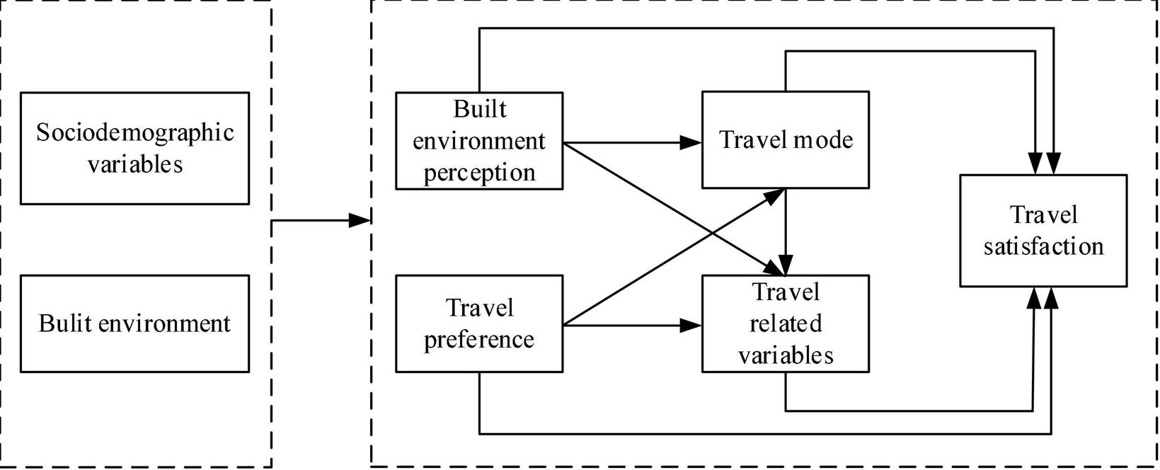
The conceptual framework.
Sample Selection and Data Collection
Sample Selection
Sichuan Province is located in the hinterland of Southwest China, with an urbanization rate of 52.29% at the beginning of 2019. With the advancement of urbanization, its rural economy is constantly improving (Ao et al., 2021). Statistics show that the construction of transportation facilities in Sichuan Province has amounted to ¥1030 billion during the 13th Five-Year Plan period, which is 1.23 times higher than the 12th Five-Year Plan period. At present, the access rate of hardened roads in the built villages1 has reached 100%, and the newly rebuilt rural roads have reached 97,000 km (Sichuan Provincial People’s Government, 2017). At the end of 2018, the total mileage of rural roads in the province has reached 286,000 km, ranking first in the country. In 2017, the Sichuan provincial government published the list of Top 100 villages to show the development of rural areas (Figure 2), in which 25 villages in Chengdu are designated.
FIGURE 2
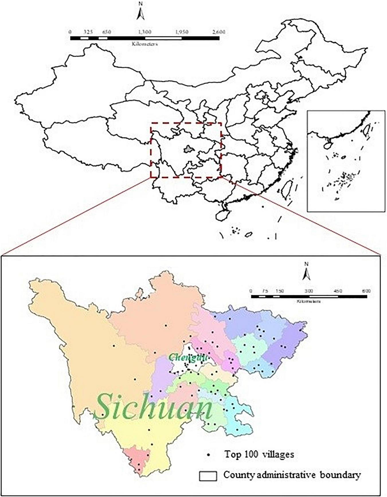
Geographic location of top 100 villages in Sichuan Province.
All Chengdu’s Top 100 villages are selected as the study area for the following two reasons: (1) Chengdu is the capital city of Sichuan Province and has transformed into a new first-tier city in China. According to the Sichuan Bureau of Statistics, the urbanization rate of Chengdu has reached 71.85% at the beginning of 2018, and it is predicted to reach 77% (Sichuan Provincial People’s Government, 2016) in 2020, which tops in the provincial list. In 2018, the regional gross domestic product reached ¥1534.277 billion (Chengdu Bureau of Statistics, 2019). The number of demonstration villages in Chengdu accounts for one-fourth of the provincial total. (2) The Top 100 villages in Chengdu are prioritized in terms of transportation infrastructure investment. Rural residents have relatively many abundant travel facilities, thereby providing a good foundation in this study. In 2019, the cumulative investment in Chengdu’s transportation infrastructure will be ¥35.322 billion, including ¥210.241 million for highway construction projects (Bureau, 2019b). Among the third batch of “four good rural roads” provincial demonstration counties in Sichuan, Chengdu has added three new demonstration county-level cities. In recent years, the mileage of rural roads in Chengdu has reached 24,795 km, and the density of rural roads has reached 172 km/100 km2. For the construction of “four good rural roads,” more than 9,800 km of new rural road reconstruction projects have been completed, covering all towns, villages, and groups in the city. In addition, Chengdu has built 61 township-level passenger stations, 253 townships, and 3,747 villages (communities) to achieve bus access, and the bus accessibility rate is 98% (Bureau, 2019a). Therefore, the Top 100 villages in Chengdu are the typical representatives of new rural development in Western China.
The selection of sample villages follows three basic principles: (1) Random selection: Twelve out of the 25 villages in Chengdu are randomly selected as basic sample villages (in the list of the Top 100 villages in Sichuan Province) (Qingshuiqiao Village, Wenquan Community, Qinggangshu Village, Wuxing Village, Shibawan Village, Youqing Community, Lianghe Village, Xingfu Village, Mingyue Village, Renhe Community, Lantian Community, and Lantiansi Village). (2) All-round coverage of geographical location: The final selected sample village needs to take the center of Chengdu (Tianfu Square) as the reference point, and the Top 100 villages as research representatives in southeast, northwest, and other directions need to be around the center. ArcGIS 10.2 is used to mark the geographical location of each Top 100 place on the map, as shown in Figure 3. The three sample villages (Hot Spring Community, Youqing Community, and Xingfu Village) in part are relatively concentrated, and the three relatively intensive sample villages are eliminated. (3) Effectively conduct the questionnaire survey into villages and households and presurvey based on the remaining nine Top 100 villages and clarify the villagers’ willingness to participate in the questionnaire survey. In accordance with the rejection degree of local residents to the questionnaire survey, three sample villages (Mingyue Village, Lianghe Village, and Renhe Community) are removed from our candidate list. Eventually, six sample villages are determined, which are located in the north of Chengdu City: Qinggangshu Village in Pidu District and Pingshuiqiao Village in Jintang County. The sample villages are Lantiansi Village in Shuangliu District in the south, Wuxing Village in Chongzhou City, Lantian Community in Dayi County in the west, and Shibawan Village in Qing Baijiang in the east. The geographical locations of sample villages are shown in Figure 4.
FIGURE 3
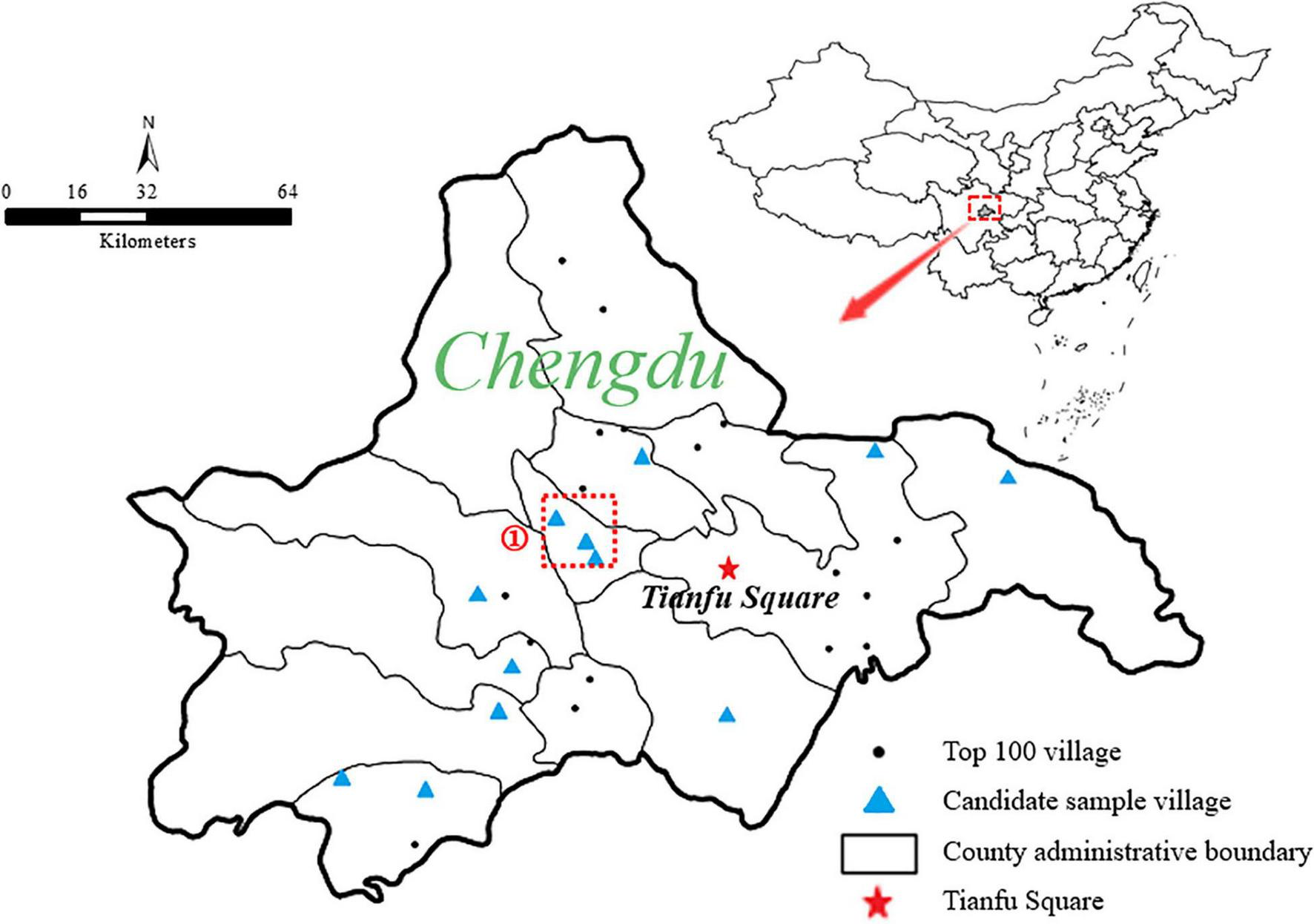
Geographical distribution of first randomly selected sample villages.
FIGURE 4
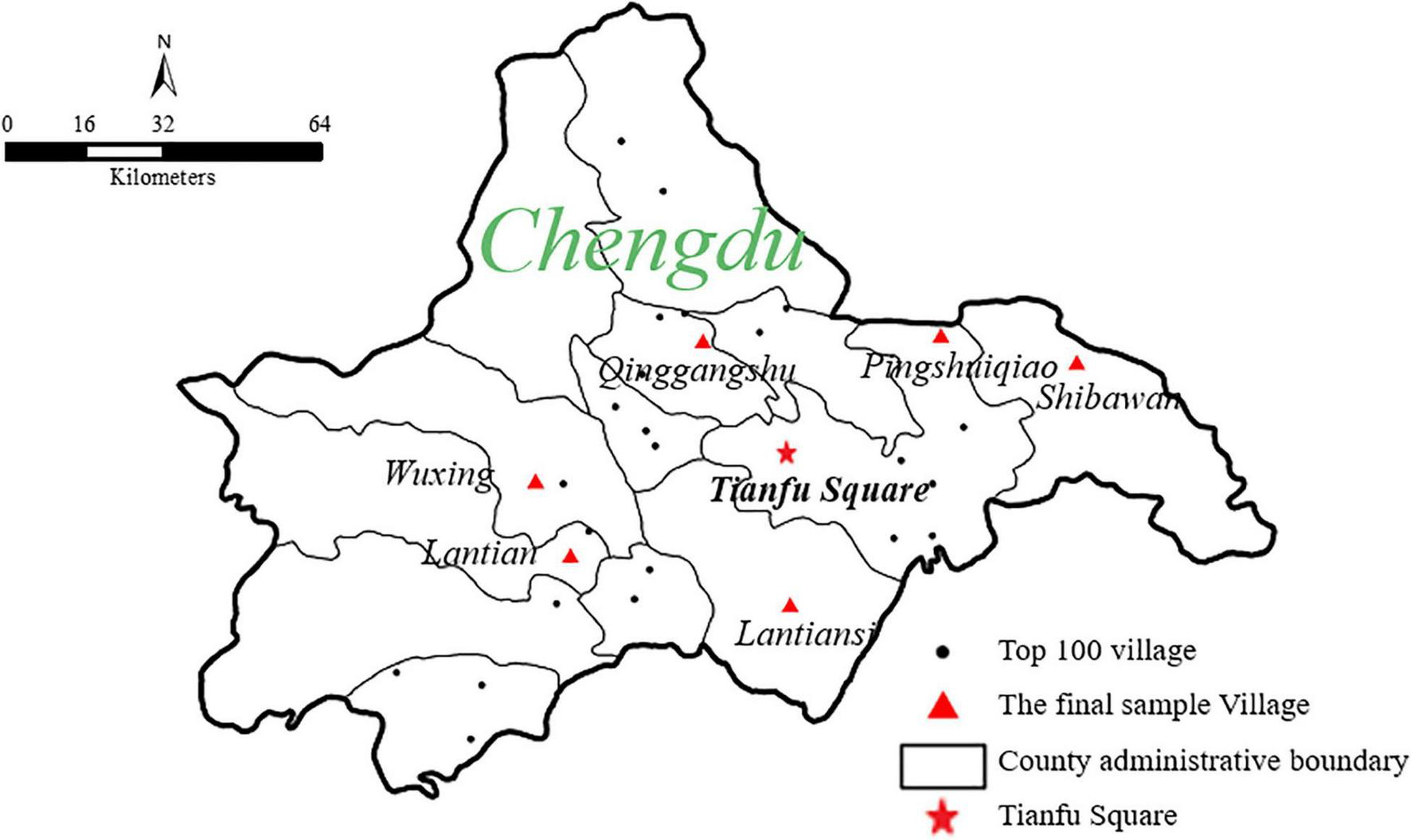
Geographical distribution of the final selected sample villages.
Data Collection
The research team recruited 12 graduate students of Chengdu University of Technology as questionnaire investigators. The research team organized questionnaire survey training and work assignment meetings to conduct an effective questionnaire survey. On the basis of the geographical location of sample villages, the researchers are divided into two teams, where each team has six people and visit three villages. During the investigation, the researchers take the village committee or the villagers’ activity center as the center for conducting a divergent visit to village residents and randomly select villagers as the research objects in conducting household investigations to ensure that the respondents are evenly distributed. Stratified sampling was used, where 50 or 100 sample households were randomly visited in sample villages of less than 1,000 households or of 1,000 to 2,000 households, respectively (Zhao and Li, 2019). In the process of filling in the questionnaire, a small number of residents did not complete the form, being interrupted by chores, visitors or being called on to fulfill other activities. The final number of investigated households is listed in Table 1. In this survey, 591 questionnaires were collected. After eliminating invalid questionnaires, 585 valid questionnaires were retained. Effective rate of questionnaire completion was 98.98%.
TABLE 1
| Village name | Total number of households in the village | Number of random survey households | Number of valid questionnaires | Effective sampling proportion |
| Wuxing | 873 | 117 | 115 | 13.17% |
| Lantian | 983 | 131 | 128 | 13.02% |
| Lantiansi | 1,209 | 103 | 102 | 8.44% |
| Qinggangshu | 932 | 80 | 80 | 8.58% |
| Shibawan | 1362 | 80 | 80 | 5.87% |
| Pingshuiqiao | 1,520 | 80 | 80 | 5.26% |
Basic data of samples.
Variable Specification
Scale of Satisfaction (STS) Variables
Scale of satisfaction is proposed by Ettema et al. (2011) and includes two levels of cognition and emotion. Nine questions are found in the STS, and each question scores from −3 to 3. The items of STS and the meaning of the scores are shown in Table 2.
TABLE 2
| Cognitive evaluation | My daily travel was worst (−3) – best I can think of (3) | |
| My daily travel was low (−3) – high standard (3) | ||
| My daily travel poorly worked (−3) – worked well (3) | ||
|
|
||
| Positive deactivation – negative activation | I feel my daily travel time is pressed (−3) – relaxed (3) | |
| I am worried that I would not be in time (−3) – confident I would be in time (3) | ||
| Emotion | I am stressed (−3) – calm (3) | |
|
|
||
| Positive activation – negative deactivation | I am tired (−3) – alert (3) | |
| Bored (−3) – enthusiastic (3) | ||
| I am fed up (−3) –engaged (3) | ||
Scale of satisfaction (STS).
On the basis of the preliminary statistical analysis, the scores of rural residents on travel satisfaction are concentrated in 0 and 1, and the proportion of negative evaluation on travel satisfaction is extremely small. The scores of each item are shown in Figure 5. The average score of STS scale is calculated and used in path analysis.
FIGURE 5
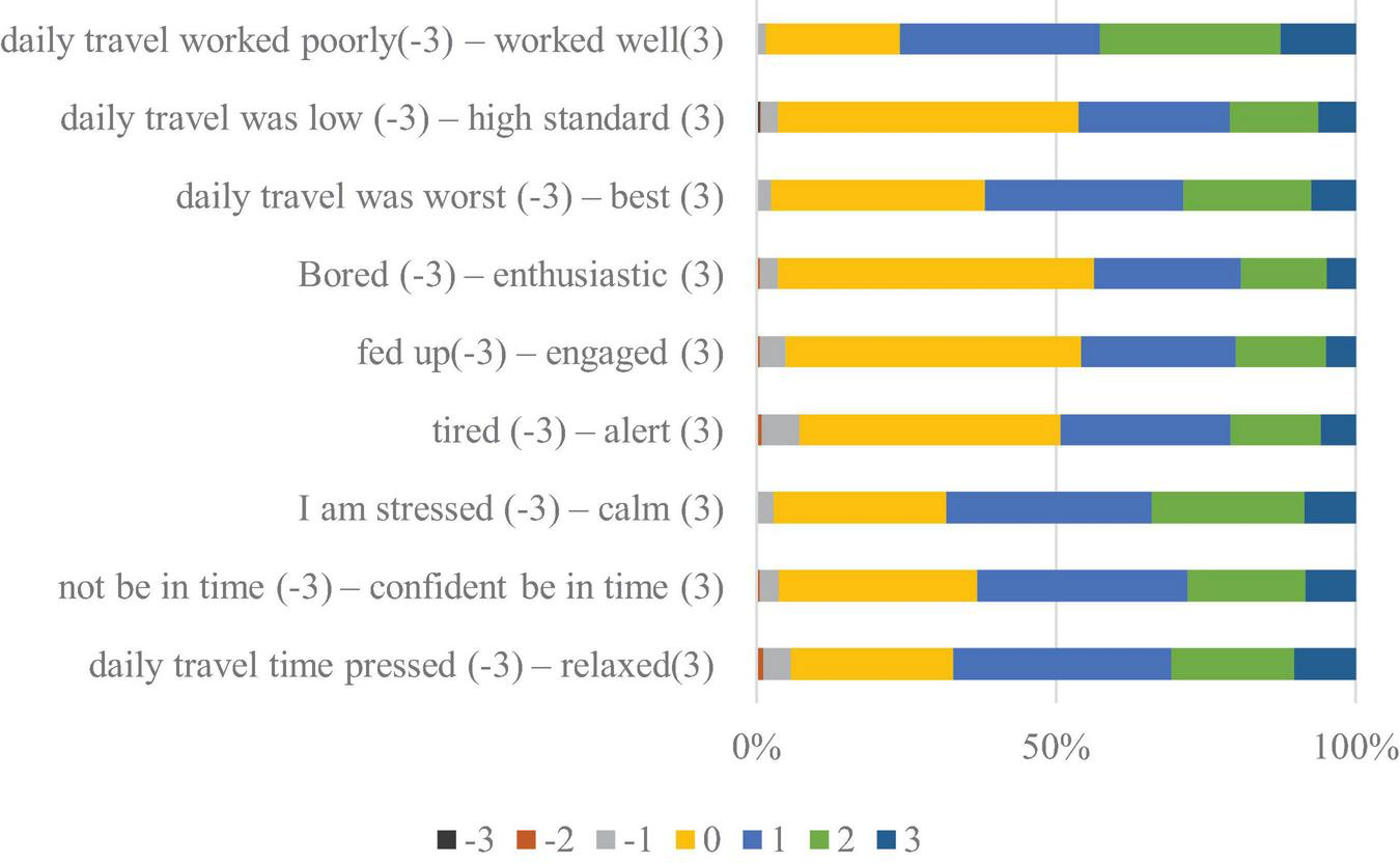
Travel satisfaction score.
Socio-Demographic Variables
Socio-demographic variables have a significant impact on residents’ travel satisfaction (Meng et al., 2013; St-Louis et al., 2014; Carrel et al., 2016; De Vos et al., 2016; Zhu and Fan, 2018a,c). Socio-demographic variables considered mainly include gender, age, registered residence type, annual personal income, education level, health status, and annual family income.
The preliminary statistical analysis shows that no significant difference is found in the sex ratio of the respondents, and 37.9% of the total respondents in rural areas are more than 60 years old. In China’s rural areas, no higher education institutions are found, students choose to study outside, and farming is the main income source. Most of the labor force prefers to work outside the home, resulting in an extremely old rural average age. Regarding the education level, respondents with a junior high school degree and below accounts for 80.2%. In the survey sample, the average education level is low because the respondents are old, and the corresponding education level is low. The highest percentage of respondents’ annual income ranges from ¥10000 to ¥50000. Among the respondents, the health condition of rural residents is good, and 96.8% of rural residents have rural registered residence. The socio-demographic variables of the respondents are consistent with the actual situation of rural areas in Chengdu. The detailed socio-demographic information of the respondents are shown in Table 3.
TABLE 3
| Variable | Frequency | Percentage | |
| Gender | Male | 285 | 48.7 |
| Female | 300 | 51.3 | |
| Annual personal income | 0 | 172 | 29.4 |
| Less than ¥10,000 | 88 | 15.0 | |
| ¥10,000–50,000 | 270 | 46.2 | |
| ¥50,000–100,000 | 43 | 7.4 | |
| ¥100,000–150,000 | 9 | 1.5 | |
| More than ¥150,000 | 3 | 0.5 | |
| Education level | Primary school and below | 301 | 51.4 |
| Junior middle school | 168 | 28.7 | |
| High school (technical secondary school) | 66 | 11.3 | |
| Junior college | 34 | 5.8 | |
| Undergraduate | 15 | 2.6 | |
| Postgraduate and above | 1 | 0.2 | |
| Health condition | Very bad | 3 | 0.5 |
| Bad | 61 | 10.4 | |
| Common | 146 | 25.0 | |
| Healthy | 254 | 43.4 | |
| Very healthy | 121 | 20.7 | |
| Registered residence type | Rural registered residence | 566 | 96.8 |
| Urban registered residence | 19 | 3.2 | |
| Annual family income | Less than 10,000 | 22 | 3.7 |
| 10,000–50,000 | 311 | 53.2 | |
| 50,000–100,000 | 197 | 33.7 | |
| 100,000–150,000 | 33 | 5.6 | |
| 150,000–200,000 | 12 | 2.1 | |
| More than 200,000 | 10 | 1.7 | |
| Age | Under 20 years old | 11 | 1.9 |
| 20–29 years old | 33 | 5.7 | |
| 30–39 years old | 52 | 8.9 | |
| 40–49 years old | 110 | 18.8 | |
| 50–59 years old | 157 | 26.8 | |
| 60–69 years old | 120 | 20.5 | |
| Over 70 years old | 102 | 17.4 | |
Socio-demographic variables.
Built Environment Variables
On the basis of existing research (Ye and Titheridge, 2017; Ao et al., 2019a,b; Zhao and Li, 2019), the built environment indexes considered in this study include building density, road density, population density, the number of accessible markets, and destination accessibility. The calculation scope of the built environment measurement index is a buffer of 1 km around the center of the village (in the activities of the village committee or residents). ArcGIS 10.2 is used to extract the data of building area and road length, and the population density and the number of accessible markets are obtained from village leaders. For the destination accessibility, the researchers used OvitalMap to locate the residents and accurately obtained the distance from the residents to the market, school, health center, and town center. Table 4 shows the built environment data of each village. The distribution of interviewees, buildings, and roads is shown in Figure 6.
TABLE 4
| Village variables | Building density | Road density | Population density | Number of accessible markets | Average destination accessibility |
| Wuxing | 0.108 | 3.958 | 0.651 | 1 | 1.097 |
| Lantian | 0.253 | 2.041 | 0.702 | 1 | 1.455 |
| Lantiansi | 0.037 | 3.050 | 0.835 | 3 | 0.856 |
| Qinggangshu | 0.079 | 2.646 | 0.478 | 1 | 2.056 |
| Shibawan | 0.088 | 2.857 | 0.757 | 1 | 1.699 |
| Pingshuiqiao | 0.047 | 3.404 | 0.992 | 1 | 1.819 |
Built environment data.
Building density = area of construction land/total area of the research area (total area of research land: take the village committee as the center and 1 km as the radius to draw a circle for determining the scope); Road density = total length of road/total area of the study area; Population density = population/total area of the study area; Number of accessible markets: obtain the actual value of the sample village; Destination accessibility = Σk{1/(dk + 1)}, k = 1, 2, 3, 4 (distance from home of respondents to market d1, school d2, health center d3, and town center d4) (Anowar et al., 2014; Ao et al., 2019b).
FIGURE 6
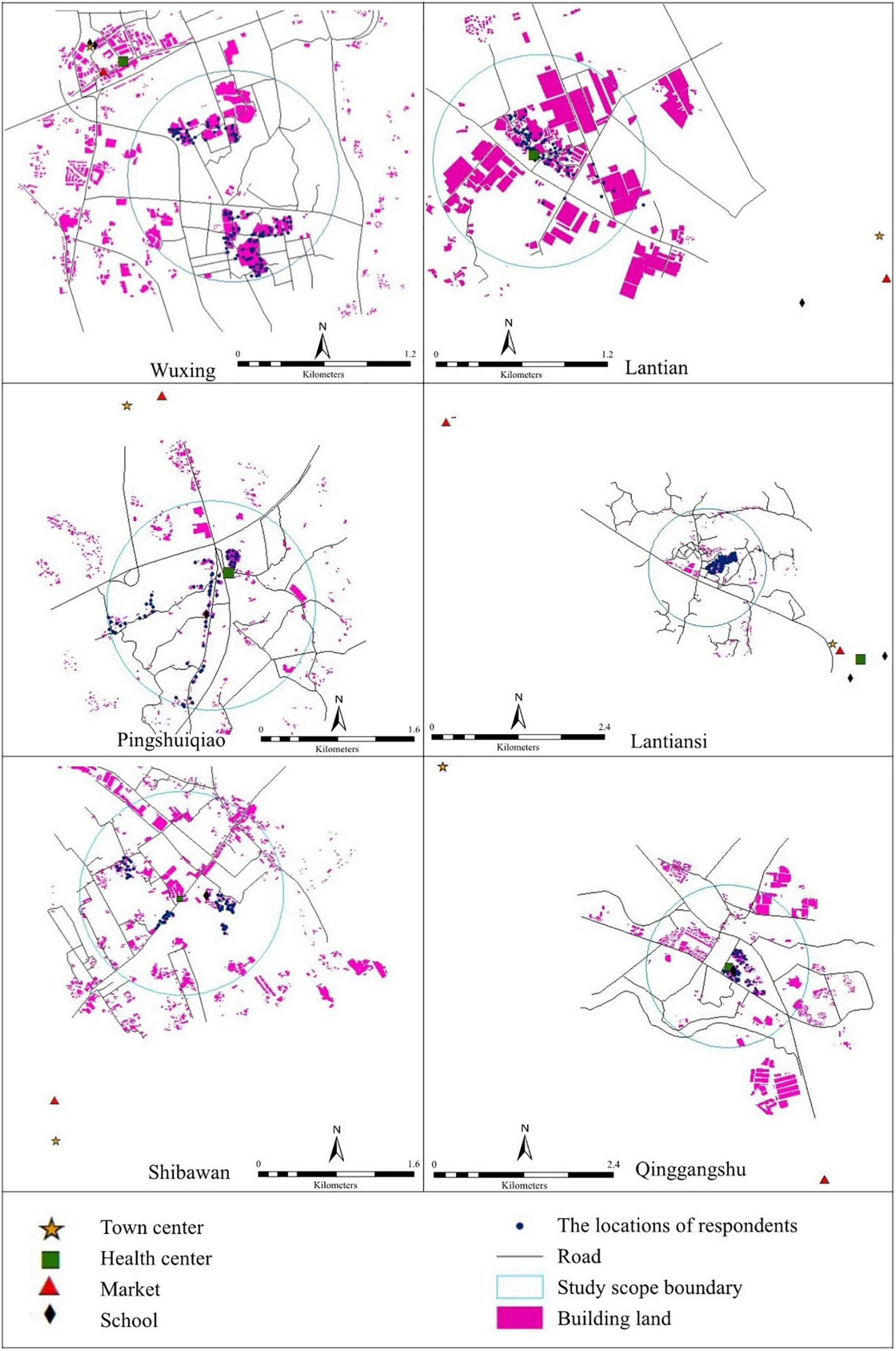
Distribution of respondents, buildings, and roads.
Built Environment Perception and Travel Preference Variables
The perception of the built environment and travel preference are mainly referenced by De Vos et al. (2016), Ye and Titheridge (2017), and Ao et al. (2019b). Five variables are used in the perception of the built environment, and eight variables are applied in travel preference. In accordance with the perception of the built environment and preference for the travel mode of the respondents, they were asked to use the five-point Likert scale for determining the degree of recognition of the 13 items from 1 to 5 (Yang et al., 2020). SPSS 23.0 is used to analyze the factors of perception of the built environment and travel preference. The results show that the p-value is 0.000, and the KMO value is 0.840, which are suitable for factor analysis. Maximum variance rotation is used to rotate the factor matrix because the initial load structure is unclear. The cumulative interpretation variance ratio of common factors is 90.061%, and two common factors, namely, accessibility perception factor and infrastructure perception, are extracted from five variables, as shown in Table 5. The result of factor analysis for travel preference shows that the p-value is 0.000, and the KMO value is 0.788. The factor matrix is rotated through maximum variance rotation, and the cumulative interpretation variance ratio of common factors is 60.472%. Two common factors, namely, prefer own transport and prefer walking and public transport, are extracted from eight variables, as shown in Table 6.
TABLE 5
| Items | Component |
|
| Infrastructure perception | Accessibility perception | |
| Good sidewalk for travel | 0.876 | 0.41 |
| Good bicycle lane for travel | 0.895 | 0.384 |
| Good motorway for travel | 0.814 | 0.454 |
| Convenient to reach the public transport station | 0.359 | 0.876 |
| The destination is accessible | 0.468 | 0.797 |
| Characteristic value | 4.042 | 0.461 |
| Variance percentage (%) | 51.563 | 38.498 |
| Cumulative variance percentage (%) | 51.563 | 90.061 |
Built environment perception: composition matrix after rotation.
TABLE 6
| Component |
||
| Items | Prefer own transport | Prefer walking and public transport |
| I like driving | 0.692 | −0.223 |
| I like to ride electric bicycle | 0.521 | 0.283 |
| I like riding motorcycles | 0.861 | −0.025 |
| I like cycling | 0.658 | 0.37 |
| I like to drive a tricycle | 0.79 | 0.06 |
| I like other modes to travel | 0.802 | 0.262 |
| I like to take public transport | 0.104 | 0.777 |
| I like walking | 0.014 | 0.832 |
| Characteristic value | 3.384 | 1.454 |
| Variance percentage (%) | 40.032 | 20.441 |
| Cumulative variance percentage (%) | 40.032 | 60.472 |
Travel mode preference: component matrix after rotation.
Daily Travel Mode Variables
The question for recording the travel mode of respondents is ‘‘what is the most common transportation to choose for your daily travel?’’ The commonly used travel modes of rural residents are electric bicycles (38.8%) and walking (24.6%). Electric bicycles have a flexible body, simple operation, and low economic burden, making them preferable by rural residents. With the improvement on the living standards of rural residents, the proportion of using cars (18.5%) ranks second to electric bicycles and walking. The probability of choosing public transport2 (6.6%), motorcycles (4.8%), tricycle (3.1%), bicycles (2.7%), and other modes (0.9%) is less than 10%.
Satisfaction With Daily Travel Mode
The respondents have been asked to use the seven-point Likert scale to express their satisfaction with daily travel mode, where 1 indicates very dissatisfied, and 7 indicates very satisfied. The results show that rural residents are fairly satisfied with their daily travel mode, with the total proportion of most satisfied (9.7%), very satisfied (34.4%), and relatively satisfied (26.0%) accounting for 70.1%, and 23.8% of them are generally satisfied with travel mode. The total proportion of dissatisfied (5.30%), very dissatisfied (0.5%), and very dissatisfied (0.3%) is only 6.1%, in which 0.3% is very dissatisfied.
Multicollinearity Test
Before path analysis modeling, the author have tested all the variables for collinearity. In this paper, variance expansion factor (VIF) is used to test the collinearity. VIF > 10 indicates serious multicollinearity between variables (Wu, 2014), thereby affecting the model fitting (Yang et al., 2019). The VIF value of the variable in this study is less than 10, as shown in Table 7. No multicollinearity is found between the variables. Thus, the path analysis in the next step can be conducted.
TABLE 7
| Variable | VIF | |
| socio-demographic factors | Gender | 1.237 |
| Age | 2.192 | |
| Education level | 2.211 | |
| Registered residence type | 1.172 | |
| Annual personal income | 2.091 | |
| Annual family income | 1.795 | |
| Health condition | 1.332 | |
| Built environment | Building density | 7.425 |
| Road density | 5.360 | |
| Population density | 1.446 | |
| Number of accessible markets | 6.168 | |
| Destination accessibility | 3.921 | |
| Travel mode satisfaction | Travel mode satisfaction | 1.478 |
| Daily travel mode | Car | 2.609 |
| Motorcycle | 1.380 | |
| Electric bicycle | 1.926 | |
| Cycling | 1.180 | |
| tricycle | 1.239 | |
| Public transport | 1.445 | |
| Other travel modes | 1.105 | |
| Built environment perception and travel mode preference | Accessibility perception | 1.417 |
| Infrastructure perception | 1.883 | |
| Prefer own transport | 1.533 | |
| Prefer walking and public transport | 1.676 |
Multicollinearity test.
Results and Discussion
In this paper, Amos21.0 has been used to build a path analysis model of influencing factors of travel satisfaction. The path relationship between the variables has been constructed and fitted in accordance with the theoretical hypothesis model in 3.1. After removing the non-significant path (p > 0.1) from the model fitting results, fitting has been conducted until all the paths are significant, and the model has been modified in accordance with the modified index (MI).
Analysis of Model Results
The p-value of the model is 0.001, which is significantly less than the test value of 0.05. Thus, the model is established. The chi-square is 275.588, and the degree of freedom (DF) is 203. The root mean square error of approximation (RMSEA) (0.025) is less than 0.05, indicating that the model has good suitability, and the comparative fit index (CFI) (0.984) is greater than 0.9, indicating that the model has a good acceptability. Chi-square statistics (CMIN)/DF, normed fit index (NFI), and increment fit index (IFI) values are all in line with the standard, and the model fitting parameters are shown in Table 8. The direct, indirect, and total Impact results of path analysis are shown in Table 9.
TABLE 8
| Model fitting index | Model fitting value | Standard value | Test result |
| CMIN/DF | 1.358 | <2.0 | Satisfactory |
| P | 0.001 | <0.05 | Satisfactory |
| RMSEA | 0.025 | <0.05 | Satisfactory |
| NFI | 0.945 | >0.9 | Satisfactory |
| CFI | 0.984 | >0.9 | Satisfactory |
| IFI | 0.985 | >0.9 | Satisfactory |
Fitting results of SEM.
TABLE 9
| Socio-demographic factors |
Built environment |
Perception of built environment and travel preference |
Travel mode |
Travel mode satisfaction | |||||||||||||||
| Education level | Annual family income | Age | Gender | Health condition | annual personal income | Number of accessible markets | Road density | Building density | Population density | Number of accessible markets | Prefer walking and public transport | Infrastructure perception | Accessibility perception | Prefer own transport | Car | Public transport | Travel mode satisfaction | ||
| Prefer walking and public transport | Total | / | / | / | / | / | / | 0.571*** | 0.568*** | 0.701*** | −0.118*** | 0.17** | / | / | / | / | / | / | / |
| Direct | / | / | / | / | / | / | 0.571*** | 0.568*** | 0.701*** | −0.118*** | 0.17** | / | / | / | / | / | / | / | |
| Indirect | / | / | / | / | / | / | / | / | / | / | / | / | / | / | / | / | / | / | |
| Infrastructure perception | Total | 0.096*** | / | / | / | / | / | 0.665*** | 0.63*** | 0.801*** | −0.21*** | 0.136*** | / | / | / | / | / | / | / |
| Direct | 0.096*** | / | / | / | / | / | 0.665*** | 0.63*** | 0.801*** | −0.21*** | 0.136*** | / | / | / | / | / | / | / | |
| Indirect | / | / | / | / | / | / | / | / | / | / | / | / | / | / | / | / | / | / | |
| Accessibility perception | Total | 0.101** | / | / | / | 0.092** | −0.084** | / | / | / | −0.305*** | −0.152*** | / | / | / | / | / | / | / |
| Direct | 0.101** | / | / | / | 0.092** | −0.084** | / | / | / | −0.305*** | −0.152*** | / | / | / | / | / | / | / | |
| Indirect | / | / | / | / | / | / | / | / | / | / | / | / | / | / | / | / | / | / | |
| Prefer own transport | Total | 0.178*** | / | −0.174*** | −0.069* | / | 0.234*** | / | / | 0.262*** | 0.093** | 0.072** | / | / | / | / | / | / | / |
| Direct | 0.178*** | / | −0.174*** | −0.069* | / | 0.234*** | / | / | 0.262*** | 0.093** | 0.072** | / | / | / | / | / | / | / | |
| Indirect | / | / | / | / | / | / | / | / | / | / | / | / | / | / | / | / | / | / | |
| Car | Total | 0.204** | 0.138*** | −0.156*** | −0.1*** | 0.057* | 0.191** | −0.029 | −0.032 | −0.037 | / | −0.014 | −0.146*** | 0.081** | / | / | / | / | / |
| Direct | 0.196** | 0.138*** | −0.156*** | −0.1*** | 0.057* | 0.191** | / | / | / | / | / | −0.146*** | 0.081** | / | / | / | / | / | |
| Indirect | 0.008** | / | / | / | / | / | −0.029* | −0.032 | −0.037 | / | −0.014 | / | / | / | / | / | / | / | |
| Public transport |
Total | / | / | / | 0.081** | 0.119*** | −0.143*** | / | −0.422*** | −0.502*** | / | −0.301*** | / | / | / | / | / | / | / |
| Direct | / | / | / | 0.081** | 0.119*** | −0.143*** | / | −0.422*** | −0.502*** | / | −0.301*** | / | / | / | / | / | / | / | |
| Indirect | / | / | / | / | / | / | / | / | / | / | / | / | / | / | / | / | / | / | |
| Other | Total | 0.088** | / | / | / | / | / | / | / | / | / | / | / | / | / | / | / | ||
| Direct | 0.088** | / | / | / | / | / | / | / | / | / | / | / | / | / | / | / | / | / | |
| Indirect | / | / | / | / | / | / | / | / | / | / | / | / | / | / | / | / | / | / | |
| cycling | Total | / | / | / | / | / | −0.125*** | 0.048 | 0.048 | 0.219*** | −0.01 | 0.014 | 0.084** | / | / | / | / | / | / |
| Direct | / | / | / | / | / | −0.125*** | / | / | 0.159*** | / | / | 0.084** | / | / | / | / | / | / | |
| Indirect | / | / | / | / | / | / | 0.048 | 0.048 | 0.059*** | −0.01 | 0.014 | / | / | / | / | / | / | / | |
| tricycle | Total | / | / | / | / | / | / | −0.06 | −0.06 | 0.173*** | 0.012 | −0.11*** | −0.105*** | / | / | / | / | / | / |
| Direct | / | / | / | / | / | / | / | / | 0.247*** | / | −0.092*** | −0.105*** | / | / | / | / | / | / | |
| Indirect | / | / | / | / | / | / | −0.06 | −0.06 | −0.074*** | 0.012 | −0.018*** | / | / | / | / | / | / | / | |
| Electric bicycle |
Total | −0.131*** | / | −0.025 | −0.01 | / | 0.033 | / | 0.109** | 0.145** | 0.013 | 0.109*** | / | / | / | 0.142*** | / | / | / |
| Direct | −0.157*** | / | / | / | / | / | / | 0.109** | 0.108** | / | 0.099*** | / | / | / | 0.142*** | / | / | / | |
| Indirect | 0.025*** | / | −0.025 | −0.01 | / | 0.033 | / | / | 0.037** | 0.013 | 0.01*** | / | / | / | / | / | / | / | |
| Motorcycle | Total | 0.004 | / | −0.017 | −0.095** | / | 0.022 | −0.148 | −0.143 | −0.155 | 0.049 | −0.029 | −0.103** | −0.134*** | / | 0.095** | / | / | / |
| Direct | / | / | / | −0.089** | / | / | / | / | / | / | / | −0.103** | −0.134*** | / | 0.095** | / | / | / | |
| Indirect | 0.004 | / | −0.017 | −0.007** | / | 0.022 | −0.148 | −0.143 | −0.155 | 0.049 | −0.029 | / | / | / | / | / | / | / | |
| Travel mode satisfaction | Total | 0.067 | 0.01 | −0.011 | −0.081** | 0.028 | −0.141*** | 0.061*** | 0.23 | 0.29 | −0.243** | −0.143*** | 0.09** | 0.284*** | 0.256*** | / | 0.072* | / | / |
| Direct | / | / | / | −0.073** | / | −0.133*** | −0.179*** | / | / | −0.095** | −0.158*** | 0.1** | 0.278*** | 0.256*** | / | 0.072* | / | / | |
| Indirect | 0.067 | 0.01 | −0.011 | −0.007** | 0.028 | −0.008*** | 0.24*** | 0.23 | 0.29 | −0.148** | 0.015*** | −0.01** | 0.006*** | / | / | / | / | / | |
| Travel satisfaction |
Total | 0.005* | 0.128*** | −0.015 | −0.033 | 0.019 | −0.112** | 0.314*** | 0.569*** | 0.609*** | −0.171 | −0.018 | 0.025 | 0.298*** | 0.278*** | 0.07* | 0.02 | −0.063* | 0.281*** |
| Direct | −0.069* | 0.125*** | / | / | / | −0.081** | 0.152*** | 0.34*** | 0.303*** | / | / | / | 0.218*** | 0.207*** | 0.07* | / | −0.063* | 0.281*** | |
| Indirect | 0.073* | 0.003*** | −0.015 | −0.033 | 0.019 | −0.031** | 0.162*** | 0.229*** | 0.306*** | −0.171 | −0.018 | 0.025 | 0.08*** | 0.072*** | / | 0.02 | / | / | |
Direct, indirect, and total impacts among variables.
***p < 0.01, **p < 0.05, *p < 0.1.
Impacts of Socio-Demographic Factors on Travel Satisfaction
As shown in Table 9, education level, annual family income, and annual personal income have a significant impact on travel satisfaction. The total impact of education on travel satisfaction is 0.005, indicating that the higher the education level, the higher the travel satisfaction. The path map of education level to travel satisfaction is shown in Figure 7A.
FIGURE 7
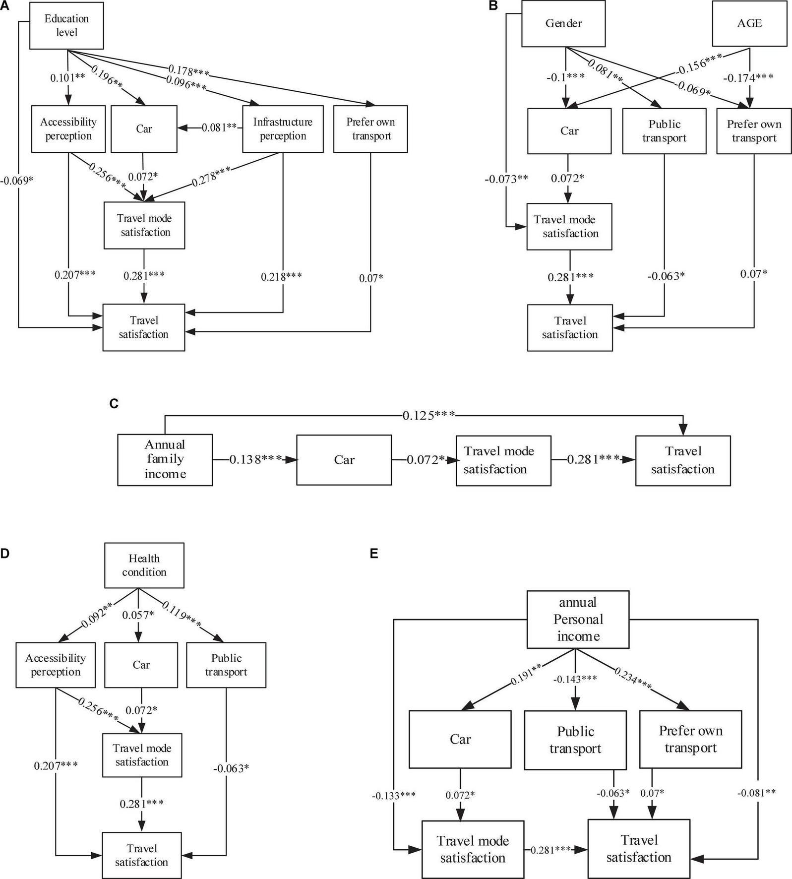
(A) Education level. (B) Gender and age. (C) Annual family income. (D) Health condition. (E) Annual personal income. ***Represents p value < 0.01, **Represents p value < 0.05, and *Represents p value < 0.1.
Regarding gender variables, the model analysis takes women as the reference group. The results show that travel satisfaction is lower for females than for males, which is consistent with previous research (St-Louis et al., 2014; Zhu and Fan, 2018c), as shown in Table 9. Chinese rural women focus more on housework, resulting in less experience in travel activities (Zhao and Yu, 2020). Less travel experience combined with low satisfaction in public transport are the reasons for their overall low travel satisfaction (Gender – Travel mode satisfaction – Travel satisfaction and Gender – Public transport – Travel satisfaction negatively affect travel satisfaction), Figure 7B.
Age has a negative indirect impact on travel satisfaction (−0.015). Table 9 shows that older adults’ satisfaction with travel is lower than that of young people, which is contrary to the conclusion of existing scholars on cities (Cao and Ettema, 2014; Gao et al., 2017a). This finding is because many older adults are found in rural areas, and the elderly have more experience in transportation facilities than do young people. Old age limits the travel options of the elderly, resulting in low satisfaction. The main negative influence path is Age – Car – Travel mode satisfaction – Travel satisfaction, as shown in Figure 7B. This path shows that the older you are, the less likely you will choose to travel by car, thereby weakening the impact on travel satisfaction.
The influence of annual family income (0.128) on travel satisfaction is positive, as shown in Table 9. The influence of annual family income on travel satisfaction is positive, as shown in Figure 7C. The higher the annual household income, the higher the satisfaction of rural residents, which is consistent with Zhao and Li (2019) conclusion. Families with good economic circumstances can afford private cars (in Figure 7C), and the impact of annual family income on private car travel is 0.138. Rural areas are far away from markets and urban areas. Thus, private car travel is convenient and fast, thereby increasing travel satisfaction.
Rural residents in good health (0.019) have high travel satisfaction, as shown in Table 9. The route map (Figure 7D) shows that residents with a better physical condition have high accessibility awareness, and the probability of choosing to drive or using public transport is high. Annual personal income has a negative impact on travel satisfaction (−0.112), as shown in Table 9. In accordance with the path map (Figure 7E), annual personal income has a negative impact through the path annual personal income – Travel mode satisfaction – Travel satisfaction, and the direct negative impact of annual personal income on travel satisfaction (−0.081) increases.
In general, the impact of social demographic attributes on travel satisfaction is small, with education notably so (0.005).
Impact of Built Environment Variables on Travel Satisfaction
Among the built environment variables, building density, road density, and the number of accessible markets have significant impacts on rural residents’ travel satisfaction (Table 9). In this study, building density has a significant positive impact on people’s travel satisfaction, and the total impact is 0.609. Rural building density represents the degree of new construction manifest in the countryside, where the increase in building density can immensely improve residents’ perception of infrastructure (0.801) and pedestrian bus preference (0.701) (Figure 8A). Change in rural urbanization and an increase in construction will improve the travel satisfaction of residents. In the study of Ye and Titheridge (2017), the built environment index has an indirect impact on travel satisfaction through travel mode and other travel variables, which is basically consistent with the conclusion of this paper.
FIGURE 8
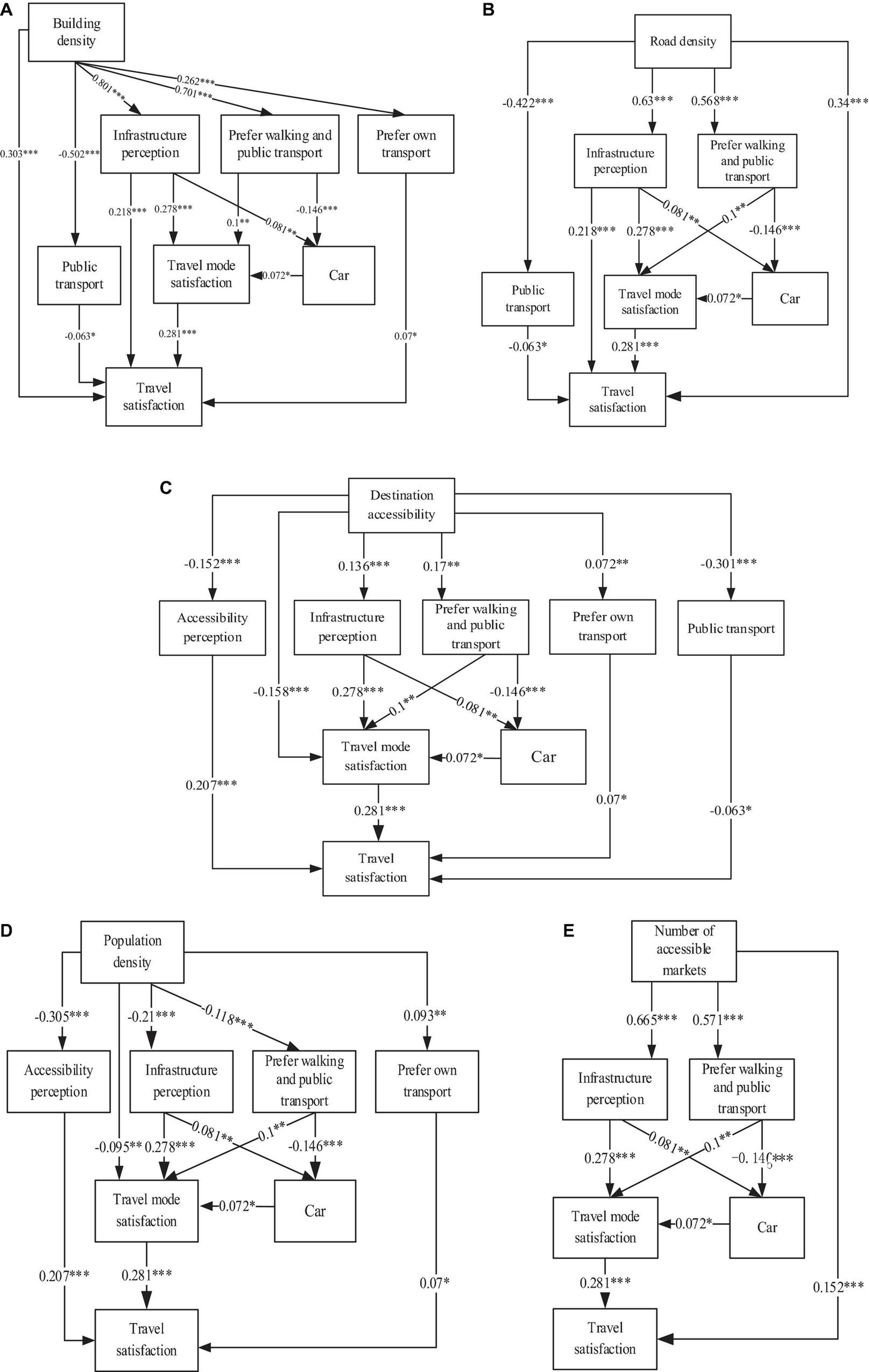
(A) Building density. (B) Road density. (C) Destination accessibility. (D) Population density. (E) Number of accessible markets. ***Represents p value < 0.01, **Represents p value < 0.05, and *Represents p value < 0.1.
The total impact of road density on travel satisfaction is 0.569, as shown in Table 9. The impact of road density on infrastructure perception is positive, with a value of 0.63 (Figure 8B). This finding shows that the greater the number of rural roads, the better people’s perception of infrastructure, and the higher satisfaction with travel. Similarly, many roads provide rural residents with greater travel convenience, where the range of travel options is greater, which can effectively improve residents’ travel satisfaction. In Figure 8B, the path Road density – Prefer walking and public transport – Travel mode satisfaction – Travel satisfaction shows that the increase in the number of roads makes greater road network density better meet people’s walking preference to improve the satisfaction of rural residents’ travel mode and travel satisfaction.
Destination accessibility does not directly affect rural residents’ travel satisfaction but indirectly affects travel satisfaction through other variables. The total impact is −0.018 (Table 9), which is contrary to the conclusion of certain scholars studying the city (Woldeamanuel and Cyganski, 2011). This condition may be explained by the following: Although the new rural built environment has objectively created better travel conditions for rural residents or has achieved the goal of destination accessibility in theory, a deviation is found from the actual accessibility perception of residents (path Destination accessibility – Accessibility perception – Travel satisfaction) (Figure 8C). Although the rural areas are still far away from the urban areas or some limitations are found in the choice of travel modes, the actual accessibility will weaken the satisfaction of rural residents to the travel modes they use, thereby causing a negative impact on travel satisfaction (path Destination accessibility – Travel mode satisfaction – Travel satisfaction) (Figure 8C).
The total impact of population density on travel satisfaction is −0.018 (Table 9). In Mouratidis et al.’s (2019) study, the impact of population density on travel satisfaction is −0.034. The impact of population density on travel satisfaction in this study is slightly smaller than that in Mouratidis et al.’s (2019) study. Travel satisfaction decreases with an increase in population density. In the path of Population density – Accessibility perception – Travel satisfaction (Figure 8D), the impact of population density on accessibility (−0.305) is negative. Although the overall travel facilities in rural areas have been improved compared with the past, the per capita ownership is very small, and many people will cause a shortage of resources and a feeling of poor accessibility (Meng et al., 2013). The number of accessible markets can reflect the convenience experienced in residents’ daily life. In this study, the number of accessible markets has a significant positive impact on rural residents’ travel satisfaction, with a value of 0.314 (Table 9). At the same time, the number of accessible markets has a positive impact on residents’ perception of infrastructure (0.665) and pedestrian bus preference (0.571), as shown in the path (Figure 8E).
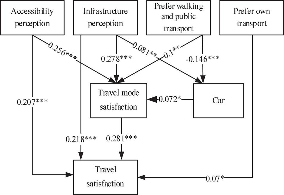
Impact of Built Environment Perception and Travel Mode Preference on Travel Satisfaction
In the built environment perception and travel mode preference, in addition to the preference for walking public transport variables, accessibility perception, infrastructure perception, and prefer own transport, have a direct positive impact on travel satisfaction, as shown in Table 9. The total effect of accessibility perception on travel satisfaction is 0.278 (Table 9). The path Accessibility perception – Travel mode satisfaction – Travel satisfaction reflects that people’s perceived accessibility will bring better travel mode satisfaction and enhance a positive impact on travel satisfaction, as shown in Figure 9. The perception of infrastructure has a positive impact on travel satisfaction, where people think that the better the sidewalks, bicycle lanes, and motorways around the living environment, the more conducive these amenities are to their daily walking, riding electric cars, and driving needs, thereby enhancing their satisfaction with daily travel mode and the impact on travel satisfaction (path Infrastructure perception – Travel mode satisfaction – Travel satisfaction) (Figure 9). Wang et al. (2020) believed that residents’ relocation to communities with good infrastructure services would improve their travel satisfaction. The preference on own transport has a direct positive impact on travel satisfaction (0.07). People who like driving tend to choose private cars and have high satisfaction (Ye and Titheridge, 2017); St-Louis et al. (2014) indicated that choosing one’s preferred mode of travel will have a positive impact on travel satisfaction, which is consistent with the conclusion of this study. Preference for walking and public transport has an indirect negative impact on travel satisfaction, where residents’ who prefer walking and public transport will reduce their driving probability. Preferring own transport has a direct positive impact on travel satisfaction (0.07) (Table 9). For example, people who prefer driving will choose private cars and have high satisfaction (Ye and Titheridge, 2017); St-Louis et al. (2014) indicated that choosing a preferred travel mode will have a positive impact on travel satisfaction, which is consistent with the conclusion of this study.
FIGURE 9
Built environment perception and travel mode preference. ***Represents p value < 0.01, **Represents p value < 0.05, and *Represents p value < 0.1.
Impact of Travel Mode and Travel Mode Satisfaction on Travel Satisfaction
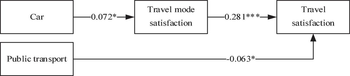
As shown in Figure 10, public transport (−0.063) has a direct negative impact on travel satisfaction, whereas driving mode has an indirect positive impact on travel satisfaction (0.020), Table 9. In this study, the five remaining travel modes, namely, electric bicycles, motorcycle, bicycle, tricycle, and other travel modes, have no significant impact on travel satisfaction (walking as reference). In the existing research on cities, walking, bicycle, private car, and other travel modes have a significant impact on travel satisfaction (Chng et al., 2016; Mao et al., 2016; Lancée et al., 2017; Zhu and Fan, 2018c).
FIGURE 10
Travel mode and travel mode satisfaction. *Represents p value < 0.1 and ***Represents p value < 0.01.
The differences between rural and urban areas may be because rural residents seldom change their travel modes in daily life and are fixed in a certain manner. In previous studies, scholars found that suburban residents are likely to choose to drive (Chen et al., 2008). For rural residents, private car travel is less time consuming and flexible, resulting in high travel satisfaction. However, the travel satisfaction of public transport is negative, which is consistent with the existing research (De Vos et al., 2016; Zhu and Fan, 2018c). China’s rural public transport is characterized by having only few modes where the service level is low (Zhao and Yu, 2020). During this research, rural residents commented that the number of rural public transport options, including small and medium-sized buses, was limited, the waiting time long, and the experience of taking public transport poor. These conditions lead to the residents’ low satisfaction in choosing public transport travel.
Conclusion and Policy Implications
Given China’s rapid development and urbanization, this paper investigates the current situation of China’s rural transportation services from the perspective of rural residents, and offers recommendations to improve travel satisfaction. This study takes the six out of the Top 100 villages of Sichuan Province in Chengdu with strong rural economic development as the research object, establishes an SEM, and studies the direct and indirect impacts of socio-demographic variables, built environment, built environment perception, travel mode preference, daily travel mode, and daily travel mode satisfaction on travel satisfaction through path analysis. The research is conducted under the special development background of China’s rural areas. The conclusions of this study are different from those of many western countries and several cities in China. The unique conclusions are summarized as follows: (1) Among the variables impacting travel satisfaction, the impact of built environment variables is the largest: the total impact of building density is 0.609; the total impact of road density is 0.569; and the total impact of the number of accessible markets is 0.314. The impact of population density and destination accessibility on travel satisfaction is indirectly negative. (2) The more satisfied the rural residents are with their travel modes, the higher their travel satisfaction. (3) In the built environment attitude and travel mode preference, infrastructure perception (0.298), accessibility perception (0.278), and the number of accessible markets (0.314) have a significant positive impact on residents’ travel satisfaction. Residents believe that the better transportation facilities around a residential area, the stronger the accessibility will be; and the greater the number of nearby markets, the higher the travel satisfaction will be. (4) The influence of socio-demographic variables on travel satisfaction is relatively low. Age (−0.015), gender (−0.033), and annual personal income (−0.112) have negative impacts on travel satisfaction, whereas education level (0.005), physical quality (0.019), and annual family income (0.128) have significant positive Impacts on travel satisfaction. (5) Among the travel mode variables, motorcycles, electric bicycles, bicycles, tricycle, and other travel modes (walking as a reference) do not affect the travel satisfaction of rural residents, which is different from many urban-based research conclusions. Rural residents’ choice of public transport as daily travel mode has a significant negative impact on their daily travel satisfaction (−0.063), whereas private car travel (0.02) has a significant indirect positive impact on their travel satisfaction.
On the basis of the above research conclusions, this paper proposes the following policy recommendations, with the aim of alleviating problems in China’s rural areas: (1) An increase in building and road densities can, to a certain extent, be expected to improve the travel satisfaction of rural residents. The construction of rural roads and transportation infrastructure should be continued, and the accessibility of destinations and amenities for residents must be improved. (2) Increase the number of convenient markets for rural residents, and the village government can open more markets near the village. (3) Rural residents’ satisfaction with public transport travel is shown to be negative, which indicates that rural public transport services must be improved. Government ought to consider appropriately increasing the frequency of rural buses services – especially small and medium-sized buses – while also adding more bus stops and in so doing shortening the distance between bus stops, augmenting existing bus routes, and increasing investment of quality of rural buses. (4) Rural built environment perception and travel preferences have a positive impact on the improvement of travel satisfaction. In considering the subjective feelings of rural residents when planning rural transportation, resident’s positive travel experience can be expected to improve.
To conclude, this study contributes in the following aspects: (1) Enrich the study of travel satisfaction in rural areas; (2) Consider the influence of subjective and objective built environment variables on travel satisfaction; (3) Identify directly the influence path of variables on travel satisfactions using a Structural equation model; (4) Generate unique insights based on the analysis; and (5) Provide targeting policy recommendations following the analysis. Our study also has some limitations. The sample villages selected in the study are the top 100 villages with good economic conditions. These villages belong to concentrated living rural areas, so they can only reflect part of the situation of concentrated living rural areas. Although rural areas are in the stage of rapid development, there is still a gap with cities, and the measurement indicators of rural built environment need to be further improved.
Publisher’s Note
All claims expressed in this article are solely those of the authors and do not necessarily represent those of their affiliated organizations, or those of the publisher, the editors and the reviewers. Any product that may be evaluated in this article, or claim that may be made by its manufacturer, is not guaranteed or endorsed by the publisher.
Statements
Data availability statement
The datasets presented in this article are not readily available because they are face to face interviews in Chinese. Requests to access the datasets should be directed to the corresponding authors where the data shall be released upon reasonable request.
Ethics statement
Ethical review and approval was not required for the study on human participants in accordance with the Local Legislation and Institutional Requirements. The patients/participants provided their written informed consent to participate in this study.
Author contributions
HL and YA: conceptualization. HL and YZ: methodology, software, data curation, and data collection. YA, YW, and TW: resources. HL, YA, and TW: writing – original draft preparation. YA, TW, and YC: writing, review, and editing. All authors have read and agreed to the published version of the manuscript.
Funding
The article processing costs are funded by the Delft University of Technology. This study was jointly supported by the National Natural Science Foundation of China (72171028).
Conflict of interest
The authors declare that the research was conducted in the absence of any commercial or financial relationships that could be construed as a potential conflict of interest.
Footnotes
1.^The villages established with the approval of provincial and municipal state organizations are called organic villages.
2.^Public transport here refers to rural buses and small and medium-sized buses in villages and towns.
References
1
Abenoza R. F. Cats O. Susilo Y. O. (2017). Travel satisfaction with public transport: determinants, user classes, regional disparities and their evolution.Trans. Res. Part A9564–84. 10.1016/j.tra.2016.11.011
2
Anowar S. Yasmin S. Eluru N. Miranda-Moreno L. F. (2014). Analyzing car ownership in Quebec City: a comparison of traditional and latent class ordered and unordered models.Transportation.411013–1039.
3
Ao Y. Chen C. Yang D. Wang Y. (2018). Relationship between rural built environment and household vehicle ownership: an empirical analysis in Rural Sichuan, China.Sustainability10:1566. 10.1007/s11116-014-9522-9
4
Ao Y. Yang D. Chen C. Wang Y. (2019a). Effects of rural built environment on travel-related CO2 emissions considering travel attitudes.Trans. Res. Part D Trans. Environ.73187–204. 10.3390/su10051566
5
Ao Y. Yang D. Chen C. Wang Y. (2019b). Exploring the effects of the rural built environment on household car ownership after controlling for preference and attitude: evidence from Sichuan, China.J. Trans. Geogr.7424–36. 10.1016/j.trd.2019.07.004
6
Ao Y. Zhang Y. Wang Y. Chen Y. Yang L. (2020a). Influences of rural built environment on travel mode choice of rural residents: the case of rural Sichuan.J. Trans. Geogr.85:102708. 10.1007/s11069-021-04632-w
7
Ao Y. Zhu H. Meng F. Wang Y. Ye G. Yang L. et al (2020b). The impact of social support on public anxiety amidst the COVID-19 pandemic in China.Int. J. Environ. Res. Public Health17:9097. 10.1016/j.jtrangeo.2020.102708
8
Ao Y. Zhang H. Yang L. Wang Y. Martek I. Wang G. (2021). Impacts of earthquake knowledge and risk perception on earthquake preparedness of rural residents.Nat. Hazards1071287–1310. 10.1016/j.jtrangeo.2018.11.002
9
Bureau C. T. (2019a). Add ‘Four Good Rural Roads’ Nation Demonstration County in Chengdu. Available online at: https://www.sc.gov.cn/10462/10464/10465/10595/2019/11/11/174c5ce193e745a8bfea5c15118833c2.shtml(accessed March 28, 2022).
10
Bureau C. T. (2019b). From January to October 2019, 35.322 Billlion Yuan has been Invested in the Transportation Infrastructure Construction of our City. Available online at: http://jtys.chengdu.gov.cn/cdjtysWap/c148686/2021-07/26/content_0396558f39f2440d8483693bf9459a87.shtml10.3390/ijerph17239097(accessed May 30, 2022).
11
Cao J. Ettema D. (2014). Satisfaction with travel and residential self-selection: how do preferences moderate the impact of the Hiawatha Light Rail Transit line?J. Trans. Land Use.793–108.
12
Cao X. Handy S. L. Mokhtarian P. L. (2006). The influences of the built environment and residential self-selection on pedestrian behavior: evidence from Austin, TX.Transportation.331–20. 10.5198/jtlu.v7i3.485
13
Carrel A. Mishalani R. G. Sengupta R. Walker J. L. (2016). In pursuit of the happy transit rider: dissecting satisfaction using daily surveys and tracking data.J. Intell. Trans. Syst.20345–362. 10.1007/s11116-005-7027-2
14
Cervero R. Sarmiento O. L. Jacoby E. Gomez L. F. Neiman A. (2016). Influences of built environments on walking and cycling: lessons from Bogotá.Urban Trans. China.3203–226. 10.1080/15472450.2016.1149699
15
Chen C. Gong H. Paaswell R. (2008). Role of the built environment on mode choice decisions: additional evidence on the impact of density.Transportation.35285–299. 10.1080/15568310802178314
16
Chengdu Bureau of Statistics (2019). Urbanization rate of Chengdu. Available online at: http://www.cdstats.chengdu.gov.cn/htm/detail_134506.html10.1007/s11116-007-9153-5(accessed February 15, 2020).
17
Chng S. White M. Abraham C. Skippon S. (2016). Commuting and wellbeing in London: the roles of commute mode and local public transport connectivity.Prev. Med.88182–188.
18
De Vos J. Mokhtarian P. L. Schwanen T. Van Acker V. Witlox F. (2016). Travel mode choice and travel satisfaction: bridging the gap between decision utility and experienced utility.Transportation43771–796. 10.1016/j.ypmed.2016.04.014
19
De Vos J. Schwanen T. Van Acker V. Witlox F. (2015). How satisfying is the scale for travel satisfaction?Trans. Res. Part F Psychol. Behav.29121–130. 10.1007/s11116-015-9619-9
20
Diana M. (2011). Measuring the satisfaction of multimodal travelers for local transit services in different urban contexts.Trans. Res. Part A.461–11. 10.1016/j.trf.2015.01.007
21
Ding C. (2007). Policy and praxis of land acquisition in China.Land Use Policy.241–13. 10.1016/j.tra.2011.09.018
22
Ding C. Lin Y. Liu C. (2014). Exploring the influence of built environment on tour-based commuter mode choice: a cross-classified multilevel modeling approach.Trans. Res. Part D Trans. Environ.32230–238. 10.1016/j.landusepol.2005.09.002
23
Eck J. R. V. Burghouwt G. Dijst M. (2005). Lifestyles, spatial configurations and quality of life in daily travel: an explorative simulation study.J. Trans. Geogr.13123–134. 10.1016/j.trd.2014.08.001
24
Etminani-Ghasrodashti R. Ardeshiri M. (2015). Modeling travel behavior by the structural relationships between lifestyle, built environment and non-working trips.Trans. Res. Part A Policy Pract.78506–518. 10.1016/j.jtrangeo.2004.04.013
25
Ettema D. Gärling T. Eriksson L. Friman M. Olsson L. E. Fujii S. (2011). Satisfaction with travel and subjective well-being: development and test of a measurement tool.Trans. Res. Part F Psychol. Behav.14167–175. 10.1016/j.tra.2015.06.016
26
Ewing R. Cervero R. (2010). Travel and the built environment: a meta-analysis.J. Am. Plan. Assoc.76265–294. 10.1016/j.trf.2010.11.002
27
Feng Z. Liu H. Zhang J. (2010). The choice model of rural population’s travel mode.J. Trans. Eng.1077–83. 10.1080/01944361003766766
28
Gao Y. Rasouli S. Timmermans H. Wang Y. (2017a). Effects of traveller’s mood and personality on ratings of satisfaction with daily trip stages.Travel Behav. Soc.71–11.
29
Gao Y. Rasouli S. Timmermans H. Wang Y. (2017b). Understanding the relationship between travel satisfaction and subjective well-being considering the role of personality traits: a structural equation model.Trans. Res. Part F Traffic Psychol. Behav.49110–123. 10.1016/j.tbs.2016.11.002
30
Kim S. Park S. Lee J. S. (2014). Meso- or micro-scale? Environmental factors influencing pedestrian satisfaction.Trans. Res. Part D.3010–20.
31
Lancée S. Veenhoven R. Burger M. (2017). Mood during commute in the Netherlands: what way of travel feels best for what kind of people?Trans. Res. Part A Policy Pract.104195–208. 10.1016/j.trd.2014.05.005
32
Li J. Xu L. Yao D. Mao Y. (2019). Impacts of symbolic value and passenger satisfaction on bus use.Trans. Res. Part D.7298–113. 10.1016/j.tra.2017.04.025
33
Li Z. Wei W. Pan L. Ragland D. R. (2012). Physical environments influencing bicyclists’ perception of comfort on separated and on-street bicycle facilities.Trans. Res. Part D.17256–261. 10.1016/j.trd.2019.04.012
34
Mao Z. Ettema D. Dijst M. (2016). Commuting trip satisfaction in Beijing: exploring the influence of multimodal behavior and modal flexibility.Trans. Res. Part A Policy Pract.94592–603. 10.1016/j.trd.2011.12.001
35
Meng B. Zhan D. S. Hao L. R. (2013). The spatial difference of residents’commuting satisfaction in Beijing based on their social characteristics.Sci. Geogr. Sin.33410–417. 10.1016/j.tra.2016.10.017
36
Mouratidis K. Ettema D. Næss P. (2019). Urban form, travel behavior, and travel satisfaction.Trans. Res. Part A.129306–320.
37
Olsson L. E. Gärling T. Ettema D. Friman M. Fujii S. (2013). Happiness and satisfaction with work commute.Soc. Indic. Res.111255–263. 10.1016/j.tra.2019.09.002
38
Sichuan Provincial People’s Government (2017). Interpretation of the Notice of the People’s Government of Sichuan Province on Printing and Distributing the “13th five year” Comprehensive Transportation Development plan of Sichuan Province. Available online at: http://www.sc.gov.cn/10462/10464/13298/13301/2017/4/10/10419613.shtml(accessed March 5, 2020).
39
Sichuan Provincial People’s Government (2016). In 2020, the Urbanization rate of Chengdu’s Permanent Population will Reach 77%. Available online at: http://www.sc.gov.cn/10462/10464/10465/10595/2016/4/21/10377147.shtml(accessed February 5, 2020).
40
Sougoubaike (2021). Countryside. Available online at: https://baike.sogou.com/v180335645.htm?fromTitle=%E5%86%9C%E6%9D%91. 10.1007/s11205-012-0003-2(accessed June 8, 2021).
41
St-Louis E. Manaugh K. Lierop D. V. El-Geneidy A. (2014). The happy commuter: a comparison of commuter satisfaction across modes.Trans. Res. Part F Psychol. Behav.26160–170.
42
Sun B. Dan B. (2015). The influence of urban built environment on residents’ commuting mode choice in Shanghai.J. Geogr.701664–1674. 10.1016/j.trf.2014.07.004
43
Susilo Y. O. Woodcock A. Liotopoulos F. Duarte A. Osmond J. Abenoza R. F. et al (2017). Deploying traditional and smartphone app survey methods in measuring door-to-door travel satisfaction in eight European cities.Trans. Res. Proc.252262–2280.
44
Turcotte M. (2011). Commuting to work: results of the 2010 general social survey.Can. Soc. Trends92, 25–36. 10.1016/j.trpro.2017.05.434
45
Wang D. Lin T. (2014). Residential self-selection, built environment, and travel behavior in the Chinese context.J. Trans. Land Use.75–14.
46
Wang F. Mao Z. Wang D. (2020). Residential relocation and travel satisfaction change: an empirical study in Beijing, China.Trans. Res. Part A Policy Pract.135341–353. 10.5198/jtlu.v7i3.486
47
Wang Y. Ao Y. Zhang Y. Liu Y. Zhao L. Chen Y. (2019). Impact of the built environment and bicycling psychological factors on the acceptable bicycling distance of rural residents.Sustainability11. 10.1016/j.tra.2020.03.016
48
Wang F. Mao Z. Wang D. (2020). Residential relocation and travel satisfaction change: an empirical study in Beijing, China. Trans. Res. Part A Policy Pract. 135, 341–353. 10.5198/jtlu.v7i3.486
49
Woldeamanuel M. G. Cyganski R. (2011). “Factors affecting traveller’s satisfaction with accessibility to public transportation,” in . Paper Presented at the Association For European Transport and Contributors 2011, (Glasgow). 10.3390/su11164404
50
Wu S. (2014). Statistical Analysis of SPSS.Beijing: Tsinghua university press.
51
Xiong Y. Zhang J. (2014). Applying a life-oriented approach to evaluate the relationship between residential and travel behavior and quality of life based on an exhaustive CHAID approach.Proc. Soc. Behav. Sci.138649–659.
52
Yan S. Gee G. C. Fan Y. Takeuchi D. T. (2007). Do physical neighborhood characteristics matter in predicting traffic stress and health outcomes?Trans. Res. Part F Traffic Psychol. Behav.10164–176. 10.1016/j.sbspro.2014.07.255
53
Yang L. (2018). Modeling the mobility choices of older people in a transit-oriented city: policy insights.Habitat Int.7610–18. 10.1016/j.trf.2006.09.001
54
Yang L. Ao Y. Ke J. Lu Y. Liang Y. (2021). To walk or not to walk? Examining non-linear effects of streetscape greenery on walking propensity of older adults.J. Trans. Geogr.94:103099. 10.1016/j.habitatint.2018.05.007
55
Yang L. Liang Y. He B. Lu Y. Gou Z. (2022). COVID-19 effects on property markets: the pandemic decreases the implicit price of metro accessibility.Tunnelling Undergr. Space Technol.125:104528. 10.1016/j.jtrangeo.2021.103099
56
Yang L. Wang X. Sun G. Li Y. (2020). Modeling the perception of walking environmental quality in a traffic-free tourist destination.J. Travel Tourism Market.37608–623. 10.1016/j.tust.2022.104528
57
Yang L. Zhou J. Shyr O. F. Huo D. D. (2019). Does bus accessibility affect property prices?Cities8456–65. 10.1080/10548408.2019.1598534
58
Yang Q. Yang Y. Yuan H. Feng Z. Ci Y. (2013). Analysis on the behavior model and influencing fators of rural residents’ travel destination selection.J. Trans. Eng.13:8. 10.1016/j.cities.2018.07.005
59
Yang Q. Yuan H. Feng S. (2014). Travel characteristics of rural residents under different economic conditions.J. Chang Univ.3476–83.
60
Ye R. Titheridge H. (2017). Satisfaction with the commute: the role of travel mode choice, built environment and attitudes.Trans. Res. Part D Trans. Environ.52535–547.
61
Zhao P. Li P. (2019). Travel satisfaction inequality and the role of the urban metro system.Trans. Policy.7966–81. 10.1016/j.trd.2016.06.011
62
Zhao P. Li S. (2018). Suburbanization, land use of TOD and lifestyle mobility in the suburbs.J. Trans. Land Use.11195–215. 10.1016/j.tranpol.2019.04.014
63
Zhao P. Yu Z. (2020). Investigating mobility in rural areas of China: features, equity, and factors.Trans. Policy.9466–77.
64
Zheng R. Chen C. (2017). Study on the travel characteristics of rural residents in Shanghai – a case study of zhoukang daju.Integr. Trans.3979–85+93. 10.1016/j.tranpol.2020.05.008
65
Zhu J. Fan Y. (2018a). Daily travel behavior and emotional well-being: effects of trip mode, duration, purpose, and companionship.Trans. Res. Part A Policy Pract.118360–373.
66
Zhu J. Fan Y. (2018b). Review of overseas studies on subjective well-being during travel and implications for future research in China.Int. Urban Plan.3374–83. 10.1016/j.tra.2018.09.019
67
Zhu J. Fan Y. (2018c). Commute happiness in Xi’an, China: effects of commute mode, duration, and frequency.Travel Behav. Soc.1143–51. 10.22217/upi.2017.402
Summary
Keywords
travel preference, travel satisfaction, rural China, travel mode, built environment
Citation
Li H, Zhang Y, Ao Y, Wang Y, Wang T and Chen Y (2022) Built Environment Impacts on Rural Residents’ Daily Travel Satisfaction. Front. Ecol. Evol. 10:931118. doi: 10.3389/fevo.2022.931118
Received
28 April 2022
Accepted
20 May 2022
Published
06 July 2022
Volume
10 - 2022
Edited by
Shaoquan Liu, Institute of Mountain Hazards and Environment (CAS), China
Reviewed by
Zhen Guo, Beihang University, China; Xin Deng, Sichuan Agricultural University, China
Updates
Copyright
© 2022 Li, Zhang, Ao, Wang, Wang and Chen.
This is an open-access article distributed under the terms of the Creative Commons Attribution License (CC BY). The use, distribution or reproduction in other forums is permitted, provided the original author(s) and the copyright owner(s) are credited and that the original publication in this journal is cited, in accordance with accepted academic practice. No use, distribution or reproduction is permitted which does not comply with these terms.
*Correspondence: Yibin Ao, aoyibin10@mail.cdut.edu.cnTong Wang, t.wang-12@tudelft.nl
This article was submitted to Interdisciplinary Climate Studies, a section of the journal Frontiers in Ecology and Evolution
Disclaimer
All claims expressed in this article are solely those of the authors and do not necessarily represent those of their affiliated organizations, or those of the publisher, the editors and the reviewers. Any product that may be evaluated in this article or claim that may be made by its manufacturer is not guaranteed or endorsed by the publisher.