Color in motion: Generating 3-dimensional multispectral models to study dynamic visual signals in animals

Introduction

For sensory ecologists interested in how dynamic visual signals are designed and how they evolve, incorporating aspects of motion and geometry into studies of animal color is a pressing goal (Rosenthal, 2007; Hutton et al., 2015; Echeverri et al., 2021). Over the years, biologists have increasingly appreciated the dynamic nature of animal colors, which can change over a range of timescales due to a variety of mechanisms (Rosenthal, 2007). Dynamic colors can be the result of physiological changes, such as the selective expansion and contraction of chromatophores that elicit rapid color changes in cephalopods (Mäthger et al., 2009; Zylinski et al., 2009) or the seasonal variation in pigmentation that allows snowshoe hares (Lepus americanus) to transition between brown summer coats and white winter coats (Zimova et al., 2018). Color change can also arise from behaviorally mediated dynamics, as in the striking courtship display of the superb bird-of-paradise (Lophorina superba) (Echeverri et al., 2021). During his display, the male maneuvers around an onlooking female, changing his position and posture to show off his brilliant plumage (Frith and Frith, 1988). As explained by Echeverri et al. (2021), the perception of colorful signals that involve behaviorally mediated color change is affected greatly by the position, distance, and direction of signalers and receivers in relation to one another as well as to the physical environment—referred to as “signaling geometry” (Echeverri et al., 2021). Today, we recognize that most animal colors are, to some degree, dynamic (Hutton et al., 2015; Cuthill et al., 2017; Echeverri et al., 2021). Despite deep interest in dynamic visual signals, the ways in which we measure color have not kept pace with our conceptual understanding of these signals. When quantifying color and pattern, researchers typically rely on static images of colorful phenotypes—ignoring certain spatial and temporal aspects of their expression. Consequently, the spatio-temporal dimensions of animal visual signals remain understudied. This is particularly true of behaviorally mediated color change, which relies strongly on aspects of motion and signaling geometry that are currently missing from most color quantification methods (Rosenthal, 2007; Hutton et al., 2015; Echeverri et al., 2021). Advances in digital imaging have made it possible for researchers to capture spectral (color) and spatial (pattern) information in static images (Chiao and Cronin, 2002; Stevens et al., 2007; Pike, 2011; Akkaynak et al., 2014; Troscianko and Stevens, 2015; Burns et al., 2017). One technique that has become a widespread and powerful tool for studying animal color is multispectral imaging. Multispectral imaging generally refers to photography in which images capture multiple channels of color information (Leavesley et al., 2005), typically including wavelengths that extend beyond the human-visible (VIS) range of light (∼400–700 nm). Recently, multispectral imaging has been used to quantify the colors and patterns of flora and fauna (Troscianko and Stevens, 2015; van den Berg et al., 2019). To be useful for objective color measurements, 2D multispectral photographs need to be calibrated to account for the wavelength sensitivity and non-linearity in the camera sensor and standardized to control for lighting conditions (Troscianko and Stevens, 2015). These calibrations produce objective, camera-independent color data that can be transformed into visual system-specific color metrics (Troscianko and Stevens, 2015)—what we refer to here as “color-accurate” information. Multispectral imaging not only allows for the collection of color-accurate information beyond the VIS range but also captures the spatial properties of patterns—providing an advantage over spectrophotometry, which measures reflectance at a small point source (Stevens et al., 2007; Troscianko and Stevens, 2015). Recently, user-friendly software has been developed for processing and analyzing multispectral images (Troscianko and Stevens, 2015; van den Berg et al., 2019), leading to increased adoption of multispectral imaging in animal coloration research. However, multispectral imaging alone is currently unsuitable for capturing motion—a common attribute of dynamic visual signals. In order to capture the relevant color information for many animal signal receivers, external filters that separately capture VIS color and color outside this range (e.g., ultraviolet or UV) are needed to photograph a scene multiple times (Troscianko and Stevens, 2015). While taking these sequential photographs, the subject must remain still so that the separate images can later be overlaid—combining all of the color information into a single image stack (Troscianko and Stevens, 2015). Consequently, this approach is unsuitable for quantifying color from freely moving animals and for capturing the 3D shape of the focal object. So, while technological advances in digital imaging have increased the spatial scale at which we can collect color information, they alone cannot capture all of the spatio-temporal dynamics of color.

Digital 3D modeling techniques offer a potential method for addressing the gaps in dynamic color analyses. In many dynamic color displays, the perceived color change is due (1) to a physiological change such as changes in blood flow, chromatophore action, pigment deposition, etc. (Negro et al., 2006; Mäthger et al., 2009) or (2) to a change in posture—such as tail-cock gestures in many Ramphastidae (toucans, toucanets, and aracaris) displays (Miles and Fuxjager, 2019)—and/or position relative to light or the signal receiver, as in iridescent bird plumage (Stavenga et al., 2011). 3D modeling is best suited to studying the second of these display types, where colors on an animal may appear inherently static but can change in appearance with respect to motion and/or angle. Digital images can be used to generate 3D representations of entire animals using photogrammetry—the science of deriving reliable 3D information from photographs (Bot and Irschick, 2019). Photogrammetric techniques, specifically Structure-from-Motion (SfM), can be used to construct a digital 3D model that is faithful to an object’s original form by combining multiple 2D images of an object taken from different angles (Chiari et al., 2008; Westoby et al., 2012; Bot and Irschick, 2019; Medina et al., 2020). Photogrammetry has been used to create 3D models from live animals (Chiari et al., 2008; Bot and Irschick, 2019; Irschick et al., 2020, 2021; Brown, 2022) as well as museum specimens (Chiari et al., 2008; Nguyen et al., 2014; Medina et al., 2020) to capture realistic 3D shape and color for the purpose of scientific application. Recently, Medina et al. (2020) developed a rapid and cost-effective pipeline for digitizing ornithological museum specimens using 3D photogrammetry. This is of particular interest to visual ecologists since birds possess some of the most diverse phenotypic variation among vertebrates, much of which can be captured by digital 3D models. While recent advances in photogrammetric software and other computer graphics tools have made generating these digital 3D models more accessible and affordable, the models produced only contain color information from the human-visible spectrum (Nguyen et al., 2014; Bot and Irschick, 2019; Irschick et al., 2020; Medina et al., 2020; Brown, 2022). This poses a problem for studying animal coloration because many organisms have visual systems sensitive to light outside this range (Delhey et al., 2015). For example, birds are tetrachromats. They possess four spectrally distinct color photoreceptors—also called “cones”—that have ultraviolet (λ_max: 355–373 nm) or violet (λ_max: 402–426 nm), shortwave (λ_max: 427–463 nm), mediumwave (λ_max: 499–506 nm), and longwave (λ_max: 543–571 nm) sensitivity (Hart and Hunt, 2007). Avian retinas also contain “double cones” (dbl), which presumably function in luminance or brightness processing in birds (Osorio and Vorobyev, 2005). Kim et al. (2012) developed a comprehensive method for producing digital 3D models of avian specimens with complete, full-spectrum information from ∼395–1,003 nm, a range spanning the near-ultraviolet to the near-infrared. However, their approach requires highly customized and often expensive equipment (3D scanners and hyperspectral cameras) and is fairly complex and computationally intensive to implement. An alternative approach, which we develop here, involves multispectral imaging in combination with photogrammetry and subsequent animation. The integration of these techniques holds great potential for studying dynamic visual signals. By combining multispectral imaging with 3D photogrammetry, we can quickly, inexpensively, and reliably reconstruct an object’s form and color, including color that is outside the human-visible range. Once a digital 3D model is constructed, it can be animated to include the behavioral components of dynamic visual signals.

Computer animation has been used in playback experiments to study animal behavior since the 1990s and continues to be a method for testing behavioral responses of live animals to complex animal stimuli (Künzler and Bakker, 1998; Chouinard-Thuly et al., 2017; Müller et al., 2017; Witte et al., 2017; Woo et al., 2017). However, in more recent years, modeling and animation have also been used to study aspects of animal form (DeLorenzo et al., 2020), locomotion (Bishop et al., 2021), and biomechanics (Fortuny et al., 2015) in silico by extracting measurements directly from digital 3D models and simulations. Recently, researchers have highlighted the promise of performing similar virtual experiments for studying colorful visual signals (Bostwick et al., 2017). Bostwick et al. (2017) illustrated how 3D modeling and animation can be a powerful tool for studying dynamic avian color using the courtship display of the male Lawes’s parotia (Parotia lawesii) as a case study. They note how 3D simulations of real-world displays can be used to address questions that are otherwise impossible to test (Bostwick et al., 2017). Specifically, they consider how virtual experiments allow researchers to manipulate aspects of a signaling interaction that are typically difficult to control in behavioral experiments. This includes various aspects of the signal phenotype, the signaling environment, and physical aspects of the signaler and receiver. For example, studying colorful signals in a virtual space lets researchers choose where to “view” a signal from by adding and adjusting virtual camera views in a simulation. The authors point out how controlling the placement of cameras in this way could improve our understanding of the display’s functional morphology since 3D computer simulations would allow them to view the male Lawes’s parotia from the precise location of visiting females (Bostwick et al., 2017). Clearly, 3D modeling and animation approaches have great potential to improve studies of dynamic animal color. However, we currently lack step-by-step workflows for producing digital 3D models containing objective color information that can be subsequently animated and analyzed in a virtual space. Here, we combine multispectral imaging with photogrammetry to produce color-accurate 3D models that include UV color information. The resulting digital 3D models produced from our workflow replicate diffuse (non-angle dependent) animal color in a virtual space. Since these digital models contain both VIS color as well as color outside this range, we call them “3D multispectral models.” Like the 2D multispectral images used to generate them, these 3D multispectral models can be analyzed from the perspective of diverse animal viewers using visual models. With the addition of animation, we can simulate the visual appearance of animal color patterns during visual displays. 3D multispectral modeling has great predictive power for investigating behaviorally mediated color change. By either replicating or manipulating postural and positional changes of signalers and receivers or conditions in the lighting environment, researchers can study the effect motion has on animal colors in a flexible virtual space. The development of this workflow will open the door to new possibilities for the study of dynamic animal colors.

Materials and methods

In this workflow, we combine multispectral imaging software—micaToolbox (version v2.2.2, Troscianko and Stevens, 2015) for ImageJ (version 1.53e, Java 1.8.0_172 64-bit, Schneider et al., 2012)—with photogrammetric software—Agisoft Metashape Professional Edition (Agisoft LLC, St. Petersburg, Russia)—to generate multispectral 3D models of four male bird specimens. These included a hooded pitta (Pitta sordida, specimen #9951), a pink-necked green pigeon (Treron vernans, specimen #17548), a summer tanager (Piranga rubra, specimen #118), and a vermillion flycatcher (Pyrocephalus obscurus, specimen #12452). All four models can be seen in VIS color in Supplementary Video 1. Specimens were from Princeton University’s natural history collection. We outline four main steps for generating multispectral 3D models: (1) image capture, (2) image processing, (3) mesh reconstruction and refinement, and (4) texture generation and refinement. The result of these steps is a 3D multispectral model. The final model for one of these specimens, the hooded pitta, is displayed in Figure 1A. Information derived from multiple 2D multispectral images (Figure 1B) produce a 3D model that accurately captures the color (see Supplementary Video 1) and 3D shape (Figure 1C) of the museum specimen.

FIGURE 1

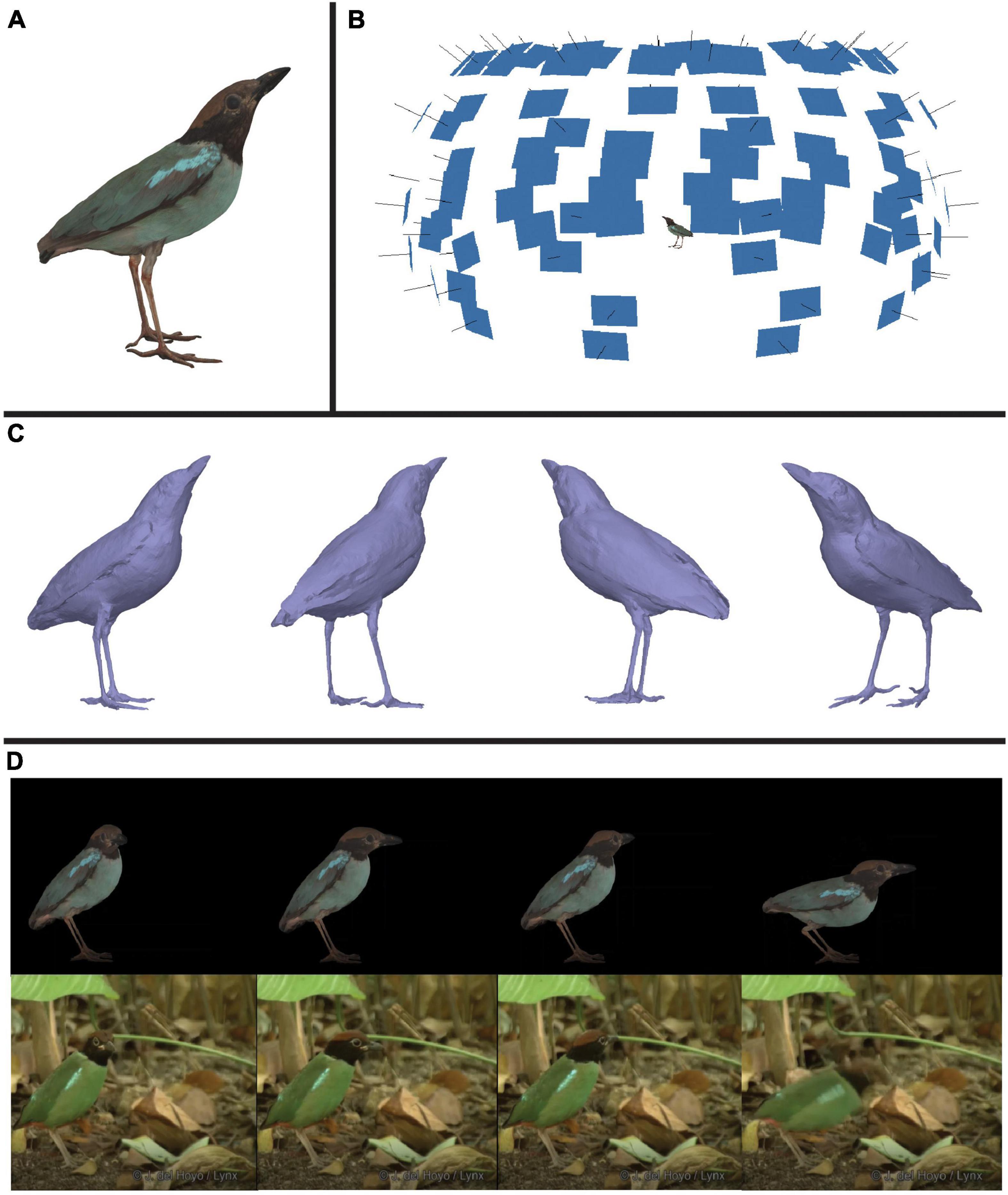
Figure 1. An illustration of one product of this workflow: a color-accurate 3D model of a hooded pitta (Pitta sordida). (A) An image of the textured model of the hooded pitta. See Supplementary Video 1 to view this model with the calibrated UV/VIS color channel textures and RGB composite texture generated in this workflow. The other three specimen models generated in this paper are also shown with RGB composite textures. (B) The hooded pitta model (center) in a hemisphere of image thumbnails used to generate the model. Each blue rectangle indicates the estimated position of the camera for each captured multispectral image. (C) The untextured hooded pitta model shown from four different angles. (D) Using rotoscoping, we animated the model of the hooded pitta. Shown above are four frames of the animated hooded pitta model matched to four frames of a video of a live hooded pitta (ML201372881) in the wild (below). This video was provided to us by the Macaulay Library at the Cornell Lab or Ornithology. See Supplementary Video 2 to view the animation and video side-by-side.

Once the multispectral 3D model is complete, color can be extracted and analyzed using image processing software such as MATLAB (Natick, Massachusetts, USA) or micaToolbox. For some applications, creating the 3D model may be the end goal. For other applications, it may be desirable to animate the 3D model using digital animation software such as Autodesk 3ds Max (Autodesk, Inc., San Rafael, California, USA). In a virtual space, an animated model might show how a colorful signal changes in appearance from different angles, or how it changes over different timescales. To demonstrate how a 3D model produced by our pipeline may be animated, we provide an example with the hooded pitta specimen (Figure 1D and Supplementary Video 2). Figure 2 is a graphical summary of the entire workflow. In the sections below, we describe the workflow in more detail. All the custom scripts and plugins described below are available on GitHub.¹

FIGURE 2

Figure 2. Flowchart briefly summarizing the 3D multispectral model workflow. Boxes 1–4 outline the steps for generating a 3D multispectral model. Boxes 5a and 5b show how the multispectral models can be analyzed in static or animated form, respectively. Each step is described in more detail in the methods. Created with BioRender.com.

Step 1: UV and VIS image capture

The first step in this workflow is to capture both the 3D structure of the specimens and the relevant UV and VIS color of their plumage using UV/VIS photography. To do this, we imaged each bird specimen from multiple angles with a modified DSLR camera. Photographs were captured in RAW format using a Nikon (Minato, Japan) D7000 camera with a Nikon Nikkor 105 mm fixed lens and consistent aperture and ISO settings. Camera settings for each specimen are available in Supplementary Figure 1. The Nikon D7000 was previously modified (via quartz conversion) to be UV- and infrared-sensitive (Troscianko and Stevens, 2015). A custom 3D-printed filter slider was used to alternate between two filters—a Baader U−Filter (320–380 nm pass) and a Baader (Mammendorf, Germany) UV/IR−Cut/L filter (420–680 nm pass)—to capture both UV and VIS color images of the specimens, respectively. Specimens were photographed under a D65 IWASAKI EYE Color Arc light (Tokyo, Japan) that had its outer coating removed to emit UV light. Most images contained a Labsphere (North Sutton, NH) 40% Spectralon reflectance standard; all other images were calibrated using standards in photographs captured under the same lighting conditions as in previous images. To capture different viewing angles of the specimen, we used a custom-built motorized turntable. This turntable was controlled by an Arduino microcontroller, which was in turn controlled using custom MATLAB scripts. The turntable was programmed to rotate 360 degrees in increments of 30 degrees, pausing at each position until both the UV and VIS images were collected. MATLAB was also used to control the camera settings and shutter button (via DigiCamControl 2 software).² Thus, the only manual tasks during image capture were alternating between the UV and VIS filters and adjusting the camera height. The camera height was adjusted after each full rotation to capture the specimen at different vertical angles. Seven different vertical positions were used, resulting in 84 unique viewing angles and 168 images of the specimen (2 images—UV and VIS—at each angle).

Step 2: Multispectral image generation and processing

After photographing the specimen, the next step of the workflow is to generate 2D multispectral images that contain color-accurate information. The UV and VIS images were used to generate multispectral images—one for each of the 84 viewing angles—using micaToolbox (Troscianko and Stevens, 2015) for ImageJ. This process linearizes and normalizes the UV and VIS images and separates them into their composite channels: ultraviolet red (UVR) and ultraviolet blue (UVB) for the UV image and red (R), green (G), and blue (B) for the visible image. Thus, each of the 84 multispectral images comprises a stack of 5 calibrated grayscale images, one for each color channel in the multispectral image. For each 2D multispectral image, the color channel images (n = 5) were exported as separate 16-bit TIFF images using a custom ImageJ plugin. These color channel images were used in Step 4 to generate 3D multispectral model textures. In addition, composite RGB images—comprising the RGB channels only—were created from the multispectral image stack; these are images that simulate human vision and are suitable for presentations and figures (Troscianko and Stevens, 2015). These RGB “presentation images” were used to reconstruct meshes in Step 3.

Step 3: Mesh reconstruction and refinement

The third step of the workflow is to produce a mesh, which is essential for capturing the 3D structure of a specimen. A mesh is the collection of vertices, edges, and faces that make up the base of a 3D model (Chouinard-Thuly et al., 2017). To reconstruct meshes in this workflow, we used the photogrammetric software Agisoft Metashape. This software requires the purchase of a license. The presentation images made using micaToolbox were imported to Metashape to reconstruct the meshes for the specimen models. Utilizing SfM, Metashape aligns images by estimating the camera positions in space relative to the focal object, based on shared features across images (Westoby et al., 2012). We inspected the alignment at this stage and removed any images that could not be aligned properly. Using this refined alignment, Metashape constructed a dense point cloud, which is a set of 3D points that represent samples of the estimated surface of the focal object. We removed any spurious points from the dense point cloud; these points represented the background or objects in the images we were not interested in reconstructing. We used the manually edited dense point cloud to reconstruct the 3D polygonal mesh. For more information on mesh reconstruction in Metashape, see the Agisoft Metashape User Manual (Professional Edition, Version 1.8). Since SfM produced 3D objects in a relative “image-based” coordinate space (Westoby et al., 2012), we also needed to scale the meshes to “real-world” dimensions. We scaled each model to the true dimensions of the specimens by using scale bars in the images or by using known measurements of structures on the specimen.

Meshes from Metashape are high-resolution polygonal models made up of randomized triangular polygons, also called “faces.” These meshes have a very high density of faces (a high polygon count) which is good for recreating accurate and detailed geometry. However, these “high-poly” models can be hard to animate (Bot and Irschick, 2019). When the model structure is deformed during the animation process, any artifacts in the randomly triangulated high-poly mesh will produce unwanted wrinkles (Bot and Irschick, 2019). Following Bot and Irschick (2019), we used InstantMesh (Jakob et al., 2015) to retopologize the models and create a simpler shape with more organized faces. Retopologizing is the process by which the faces on the mesh are changed by reducing the face count, swapping the polygon type (e.g., from triangular polygons to quad polygons), and adjusting the edge flow, which smooths and aligns faces with the natural curvature of the specimen (Bot and Irschick, 2019). This process results in better-looking deformations during animation (Bot and Irschick, 2019). However, care should be taken when decimating and smoothing the model so that important features and measurements are not lost or changed during the process (see Veneziano et al., 2018).

Step 4: Multispectral texture generation and refinement

Having produced a mesh, the next step is to generate 3D multispectral model textures that contain the color-accurate information captured by the 2D multispectral images. A texture is a 2D projection of the color information associated with a 3D model. Pixel values from multiple images are either selected or averaged together to generate the final pixel values in the model texture. How these pixels are combined depends on the blending model selected. We used mosaic blending to generate the textures in this workflow. Mosaic blending uses a weighted average based on the position of the pixel relative to the orientation of the camera (see Agisoft Metashape User Manual, 2022). A potential benefit to the mosaic blending model is that it may reduce the effect of highlights and shadows present in the UV/VIS images (Brown, 2022). Mosaic blending highly weights pixels that are orientated straight toward the camera—which are typically well-lit areas of the images—and down-weights pixels at extreme angles—typically where shadows occur in the images. This should mean that color in the model texture will be more representative of specimen color under well-lit conditions.

Bot and Irschick (2019) compare textures to sewing patterns, which are 2D templates for garments that are sewn together to fit a 3D surface. As in the sewing pattern analogy, we can define how the projection is laid out and where we “cut” the 3D object, so that it lies flat on one plane with minimal stretching (Bot and Irschick, 2019). When the texture is wrapped back onto a 3D surface, the places where the cuts meet are called the “seams.” This projection is stored as a “UV-Map.” U and V are the height and width coordinate dimensions that inform the program where color should be placed on the model (Chouinard-Thuly et al., 2017; Bot and Irschick, 2019), not to be confused with UV (ultraviolet). In this workflow, textures are stored as 16-bit TIFF image files to retain the uncompressed color information from the 2D multispectral image stacks. UV-Maps generated in Metashape use projections with automatically generated seams that break textures into many small fragments that can be difficult to identify as specific areas on the model. We re-made the UV-Maps (initially generated from Metashape) in Autodesk 3ds Max to generate mappings with larger fragments corresponding to easily recognizable features on the specimens (e.g., parts of the wing or tail).

After both the mesh (Step 3) and texture (Step 4) were refined, we imported the new mesh and texture UV-Maps back into Metashape. We used these as a template to create the final, color-accurate 3D multispectral model textures for each specimen model. To do this, we generated a custom-Python script that swapped the presentation images in Metashape used to reconstruct the mesh (Step 3) for the color channel TIFF images (Step 2). This generated five textures—UVR, UVB, R, G, B—using the new UV-Maps, resulting in calibrated textures for all channels of UV/VIS color information. At this point in the workflow, the multispectral model has been generated and can now be used for subsequent color analyses. Color values may be extracted from the multispectral model directly (Step 5a) or the model may be animated first to add behavioral data (Step 5b) before measuring color.

Step 5a: Extracting color data directly from model textures

The output of Steps 1–4 is a 3D multispectral model. Color can be directly extracted from the textures of the 3D multispectral model using multispectral imaging software such as micaToolbox (Troscianko and Stevens, 2015). 3D multispectral model textures can be converted into images that have visual system-specific color values using cone catch models in micaToolbox (Troscianko and Stevens, 2015). These cone catch models estimate cone stimulation values for a given visual system and lighting environment. The textures may be transformed using cone mapping models that correspond to di-, tri-, and tetrachromatic animal color vision systems (Renoult et al., 2017) or using a human-centric color space like CIE XYZ (Smith and Guild, 1931). We generated a custom plugin for micaToolbox (Troscianko and Stevens, 2015) to convert the separate channel textures to a “texture” image stack that is compatible with other micaToolbox plugins. By directly extracting color measurements from 3D multispectral models, as described here in Step 5a, we tested the color accuracy of the 3D multispectral models for each bird specimen (see section “Verifying the accuracy of color information from the multispectral models”).

Step 5b: Rigging and animation

3D multispectral models generated in Steps 1–4 can also be animated (Step 5b) before color information is extracted from the model textures (Step 5a). Such animations require a mesh, a texture, and a rig (Chouinard-Thuly et al., 2017). As explained above, the mesh is the underlying 3D structure of the 3D model. The mesh holds the texture—the color and pattern information associated with the 3D model. A rig is a skeletal structure that can be manipulated to deform and move the model (Bot and Irschick, 2019). We rendered one of our 3D multispectral models—the hooded pitta—to demonstrate how to combine dynamic behavioral data with color-accurate data embedded in the 3D multispectral models using animation. Rendering is the process of generating either a still image or an animation from a raw model (Chouinard-Thuly et al., 2017). The rendering process can involve adding virtual cameras to a scene to alter views of the model as well as adding special effects to create aspects of lighting and motion. In 3ds Max, we created a basic rig based on a simplified generic bird skeletal structure to manipulate the model during animation. We used a video of a naturally behaving bird as our reference video for the animation. Specifically, we obtained a video of a hooded pitta (ML201372881) from the Macaulay Library at Cornell University. The video shows a male bird jumping out of frame. We animated the hooded pitta using a method called rotoscoping—an animation technique where a reference video is used to guide the animation of a model (Gatesy et al., 2010). This involves deforming the 3D model to match the pose of a target object in the reference video in select frames, called “key frames.” To generate the final animation, we matched frames from the Macaulay Library video at a few key frames marking the beginning and end of major pose changes throughout the video and had 3ds Max interpolate the rest of the 3D model’s movement between these key frames. Once the 3D multispectral model is animated, color information can then be extracted from stacked frames of the rendered animation similar to the way in which color is extracted from static 2D multispectral image stacks or static 3D multispectral model texture stacks (Step 5a). However, now motion is incorporated in the images used for color quantification. We are still refining this stage in the workflow, but the animation presented here (Figure 1D and Supplementary Video 2) demonstrates how we are moving toward completing this step.

Verifying the accuracy of color information from the multispectral models

In order to verify that color information has been accurately captured and retained through each of the steps from imaging (Step 1) to final texture generation (Step 4), we estimated color from several plumage patches on each 3D multispectral model (Step 5a). We first confirmed that the colors were similar to those of the same patches generated from the original 2D multispectral images (Step 2), then independently compared them to values estimated using spectrophotometry. The rationale for confirming color values using estimates from 2D multispectral images was to ensure that color from the original images was retained during the 3D multispectral model generation process. We expect the cone catch values estimated from the 3D multispectral model textures to be similar, if not identical, to values estimated from the 2D multispectral images since any view from the 3D multispectral model in effect acts as a 2D multispectral image. However, the blending process during texture generation in Step 4 could alter the color captured from the original 2D multispectral images. By verifying that the cone catch estimates from the 3D multispectral texture were similar to estimates from the original 2D multispectral images (Steps 1 and 2), we could confirm that color information was not being lost or considerably changed during the workflow. The rationale for comparing model cone catches to estimates from spectrophotometry data was to verify that the 3D multispectral models were a reasonably accurate representation of color on the original specimens. Unlike values estimated from the 2D multispectral images, cone catches estimated from the spectrophotometry data acted as an independent estimate of color that we could use to test the color accuracy of the 3D multispectral models.

To validate color measurements in the 3D multispectral models, we used the UV-sensitive visual system of the Eurasian blue tit—Cyanistes caeruleus (Hart et al., 2000). Avian visual systems are thought to be generally similar to one another outside variation in the SWS1 cone type, which can be either violet- or UV-sensitive (Hart and Hunt, 2007). Therefore, the blue tit visual system is likely comparable to other UV-sensitive avian visual systems. We generated cone catch values for 1–2 plumage patches on each specimen using three methods: 3D multispectral modeling, 2D multispectral imaging, and spectrophotometry. Samples were taken from the breast and shoulder patch on the hooded pitta, the breast and shoulder patch of the pink-necked green pigeon, the breast of the summer tanager, and the breast of the vermillion flycatcher. Icons in Figures 3, 4 show the general location of color measurements for each plumage patch. For the blue tit visual system, cone catch values represent stimulation of the ultraviolet (uv), shortwave (sw), mediumwave (mw), longwave (lw), and double (dbl)-sensitive cone types. For each 3D multispectral model, we selected small regions of interest (ROIs) using Metashape. The ROIs consisted of one small area within a plumage patch. Color can be quite variable within a plumage patch. For example, both the shoulder and breast patch on the hooded pitta contained some intra-patch variation, producing slightly different cone catch estimates when color was sampled from multiple locations within each patch (Supplementary Figure 1). To attempt to limit the effect of color variation within plumage patches, we sampled only small ROIs on the 3D multispectral texture and 2D multispectral image so that we could make relatively direct comparisons with the point source measurements collected using a spectrophotometer. For each ROI, we generated binary (black and white) masks for both the 3D model texture and all initial 2D multispectral images.

FIGURE 3

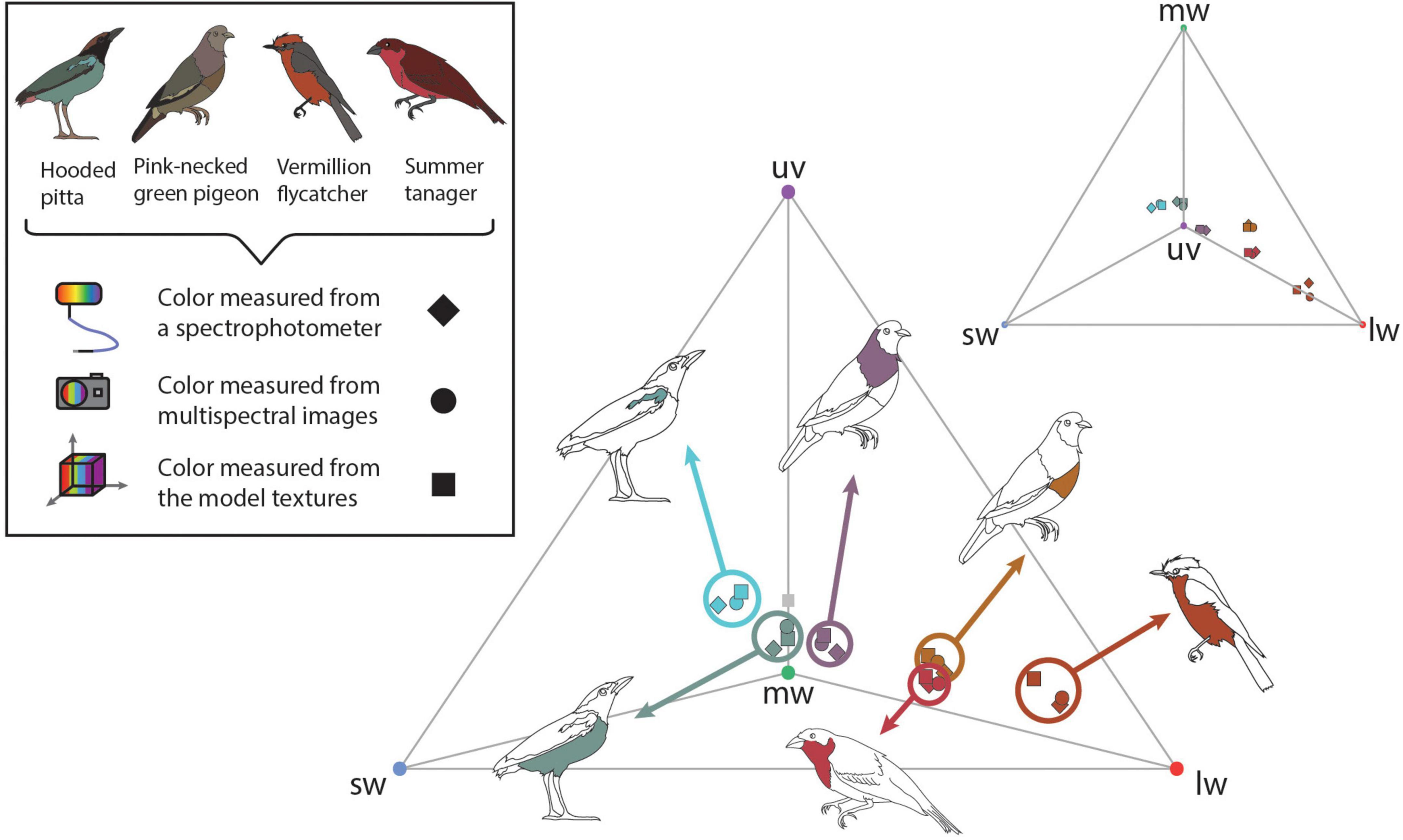
Figure 3. To validate the color information on the 3D multispectral models, we compared cone catch values extracted from 3D multispectral model textures, 2D multispectral images, and reflectance spectra. Here these cone catch values are plotted in an avian tetrahedral color space (Endler and Mielke, 2005; Stoddard and Prum, 2008). All avian visible colors can be plotted in the tetrahedral color space according to their relative stimulation of each color cone type in avian retinas, where more saturated colors fall closer to the vertices of the tetrahedron. Vertices of the tetrahedron are colored according to the cone type represented: uv (purple), sw (blue), mw (green), and lw (red). Scattered points show the color of patches estimated from the 3D multispectral model texture (squares) 2D multispectral imaging (circles), and spectrophotometry (diamonds). Bird illustrations indicate the plumage patch from which each set of color measurements was collected.

FIGURE 4

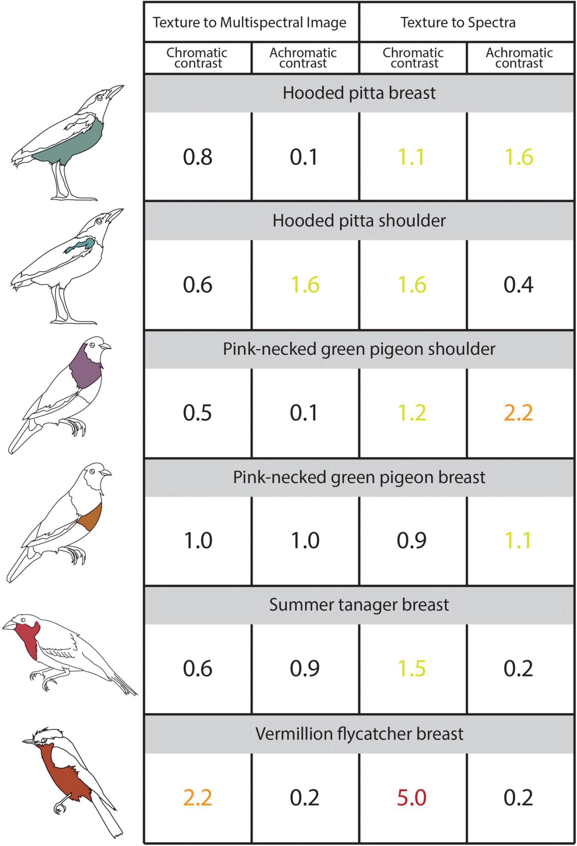
Figure 4. The illustrated table shows the chromatic and achromatic contrast values for the sampled plumage patches estimated using 3D multispectral model textures, 2D multispectral images, and reflectance spectra. Contrast values < 1 indicate that two patches are indistinguishable from one another and contrast values < 3 indicate that two colors are similar to one another. The contrast values compare colors sampled from the 3D multispectral model textures to the 2D multispectral images (Left: “Texture to Multispectral Image”) and colors sampled from 3D multispectral model textures and the reflectance spectra (Right: “Texture to Spectra”). Icons to the left of the table indicate the specimen and patch to which the values correspond. Chromatic and achromatic contrast values are colored as follows: < = 1 (black), between 1 and 2 (yellow-green), between 2 and 3 (orange), > 3 (red). See the main text for details.

Using micaToolbox (Troscianko and Stevens, 2015), we estimated the average cone catch values for all ROIs from both the model texture and one of the 84 multispectral images where the sampled patch was visible and facing directly toward the camera (i.e., similar to the image taken if only 2D multispectral images of the specimen were obtained). We also obtained reflectance spectra corresponding to the sampled plumage patches. We used a USB4000 UV-VIS spectrophotometer connected to a PX-2 pulsed xenon lamp with a ¼ inch bifurcated reflectance probe from Ocean Optics (now Ocean Insight) and the OceanView software (Ocean Insight, Dunedin, FL, USA). Three replicate reflectance measurements were collected at a 90°/90° incident light/viewing angle orientation, which were averaged to generate a single reflectance spectrum for the ROI for each patch. Color sampled using the multispectral models, multispectral images, and reflectance spectra were all converted to avian color space using the blue tit receptor sensitivities under D65 light either in micaToolbox (Troscianko and Stevens, 2015)—for the multispectral models and multispectral images—or in R (version 4.0.2, R Core Team, 2017) using the R package pavo (version 2.7.0, Maia et al., 2019)—for the reflectance spectra. To aid comparison, the D65 illuminant spectrum from micaToolbox was used for both analyses. All cone catch values estimated from the 3D multispectral textures, 2D multispectral images, and reflectance spectra were plotted in avian color space (Endler and Mielke, 2005; Stoddard and Prum, 2008) using pavo (Maia et al., 2019). This allowed us to evaluate the degree to which colors estimated using the three methods were similar (Figure 3).

We calculated noise-weighted Euclidean distances—chromatic and achromatic contrast values—to quantify the differences between color values estimated from the 3D multispectral texture, the 2D multispectral images, and the spectra. Pavo (Maia et al., 2019) generates chromatic contrast values using Vorobyev and Osorio (1998) receptor noise limited model (RNL) of vision, which correspond to an estimate of the distance between colors in terms in hue and saturation with noise based on relative photoreceptor densities (see CRAN documentation: White et al., 2021). These values are similar to the just-noticeable difference (JND), which is a contrast threshold that also uses the RNL model to estimate discriminability between two colors based on their distance in color space (White et al., 2021). Two colors that are one (or more) JNDs apart are considered to be discriminable given the assumptions of the model (Maia and White, 2018). Because of uncertainty introduced into the application of the RNL model by unknown (and assumed) variables, it is common to use a more conservative assumption that colors that are 3 or more JNDs apart are discriminable (Gómez et al., 2018; Maia and White, 2018). Noise-weighted Euclidean distances correlate with the threshold of discrimination for JNDs, so we use the JND discrimination threshold here and assume that chromatic contrast values of 3 or below are similar (White et al., 2021). Achromatic contrast values are simple (Weber) contrast values based on a Weber fraction for brightness discrimination (White et al., 2021) and similar to chromatic contrast two colors can be considered similar if the chromatic contrast between them lies between JND = 0 and JND = 3 (Siddiqi et al., 2004). To calculate chromatic and achromatic contrast, we used a cone ratio of 1 : 2 : 2 : 4 (Maia et al., 2019), a Weber fraction of 0.1 for chromatic contrast (Silvasti et al., 2021) and a Weber fraction of 0.18 for achromatic contrast (Olsson et al., 2018).

Additionally, we performed a supplementary analysis following Troscianko and Stevens (2015) to test color reproduction in our workflow. We compared cone catch values for 36 artist pastels using both our 3D multispectral modeling workflow and spectrophotometry (Supplementary Figure 2). As above, cone catches were estimated using the blue tit visual system under D65 light. Values corresponding to each cone in the blue tit visual system were correlated to assess the fit between the values estimated using our novel workflow (3D multispectral modeling) and values estimated using spectrophotometry. This allowed us to test the performance of our workflow on highly diffuse, saturated, and uniform colors without the added complexities of natural colors, such as the gloss, iridescence, and intra-patch variation that are often present in avian plumage. The results of this analysis are summarized in Supplementary Figure 2.

Results

We generated 3D multispectral models of four museum specimens that contain UV and VIS color information (Figure 1A). Cone stimulation values—uv, sw, mw, lw, and dbl cone values—were extracted from the plumage patches on each multispectral model texture. Cone stimulation values were also estimated using two standard methods for quantifying color: 2D multispectral imaging and spectrophotometry. Figure 3 shows the cone stimulation values from each method plotted in tetrahedral color space from two perspectives—one viewing the color space through the uv, sw, and lw face to show variation along these axes (center) and one looking down through the uv axis to show variation along the sw, mw, and lw axes (top right). Chromatic and achromatic contrast values that compare (1) the multispectral model textures to the multispectral images and (2) the multispectral model textures and reflectance spectra are shown in Figure 4. The results of this analysis were repeated with a more conservative Weber fraction of 0.05 and are available in Supplementary Table 2. This value is generally used for color discrimination on an achromatic background but might produce overly high color discrimination thresholds for more natural conditions (Silvasti et al., 2021). The results of this supplemental analysis are similar to the results of the main paper, which are discussed in more detail below.

Chromatic agreement

Cone catch values estimated using each method—3D multispectral models, 2D multispectral imaging, and spectrophotometry—for each ROI appeared to closely cluster in the tetrahedral color space (Figure 3). In most cases, points representing multispectral textures and multispectral images clustered more closely to each other than to the points representing the reflectance spectra. This was supported by the chromatic contrast values reported in Figure 4. Chromatic contrast values between plumage colors estimated from the multispectral model textures and the multispectral images were generally less than or equal to 1.0 (Figure 4). The breast patch of the vermillion flycatcher had the highest chromatic contrast value of 2.2, indicating that the 3D multispectral model textures and 2D multispectral images generated slightly different cone catch values. The chromatic contrast values for plumage colors estimated from the 3D multispectral model textures and reflectance spectra were also less than 2, with the exception of the contrast value for the breast patch of the vermillion flycatcher. The vermillion flycatcher had a value of 5.0 (Figure 4), indicating that the 3D multispectral model textures and reflectance spectra generated discriminably different cone catch values (JND > 3) for this specimen’s red breast patch. In general, 3D multispectral models, 2D multispectral images, and reflectance spectra produced similar cone catch estimates for specimen plumage color.

Achromatic agreement

Achromatic contrast values between the plumage colors estimated from the 3D multispectral textures and the 2D multispectral images were all less than 2 (Figure 4). The shoulder patch of the hooded pitta had the highest achromatic contrast value of 1.6 (Figure 4), while all other patches had values less than or equal to 1.0. This indicates that the 3D multispectral model textures and the 2D multispectral images generate very similar double cone estimates for most plumage patches, except for the hooded pitta shoulder patch. The achromatic contrast values for plumage colors estimated from the model textures and the reflectance spectra were also all less than 2, with the exception of the contrast value for the breast patch of the pink-necked green pigeon. This had a value of 2.2., indicating that 3D multispectral model textures and reflectance spectra generated slightly different double cone estimates, but none that were discriminably (JND > 3) different (Figure 4). Thus, in general, 3D multispectral models, 2D multispectral images, and reflectance spectra produced similar double cone estimates for specimen plumage color.

Discussion

Using multispectral imaging and photogrammetry, we developed and applied a new workflow to generate 3D models of bird specimens with objective color information that extends beyond the VIS range. To our knowledge, this is the first workflow to combine multispectral imaging techniques with photogrammetry to produce 3D models that contain UV and VIS color information. This—along with other tools and pipelines being developed in parallel—marks an important step in designing new methods for studying dynamic colorful signals. These 3D models are data-rich representations of color that can be used—even in their static form—to expand the possibilities of color analyses. As expressed by Medina et al. (2020), workflows that utilize 3D photogrammetry have an immediate and promising future in color analysis because they allow for the integration of techniques that have been optimized for color capture—in this case, multispectral imaging. Specifically, this workflow can be used to simulate changes of diffuse animal color as result of motion. With further development, this workflow has great potential to expand to applications that address many other forms of dynamic color. Below, we discuss important considerations and limitations when generating 3D models, and we expand on the applications of multispectral 3D models in both static and dynamic forms.

Workflow validation

Our results support that the 3D multispectral models generated from our workflow are a promising new mode of accurate, objective color measures. Our results show that colors estimated from 3D multispectral models are similar (in terms of cone catch values) to those estimated from 2D multispectral imaging and spectrophotometry for diffuse avian color. Specifically, the chromatic and achromatic contrast values estimated from 3D multispectral model textures and 2D multispectral images all had values under the discrimination threshold of JND = 3.0 in a receiver-specific (blue tit) color space (Figure 4). In fact, most color differences fell below the more conservative discrimination value of JND = 1 (Figure 4), suggesting that the cone catch estimates generated from 3D multispectral models and 2D multispectral images are very similar. This is unsurprising, since the 2D multispectral images are used to generate the 3D multispectral model textures. These results suggest that color from the 2D multispectral images is being conserved in the 3D multispectral model despite the pixel averaging that occurs during the 3D multispectral texture generation process (Step 4).

When compared to colors estimated from reflectance spectra, those estimated from 3D multispectral models generally resulted in higher contrasts (more difference). However, chromatic and achromatic contrasts were typically below the discrimination threshold of JND = 3.0, suggesting that the color values estimated from the 3D multispectral model textures were similar to those estimated using spectrophotometry. These two approaches (3D multispectral models vs. reflectance spectra) are unlikely to generate identical color cone estimates due to human error when trying to match the area sampled by the ROIs (using a 3D multispectral model) to an area on the physical specimen (using spectrophotometry). For example, the largest color difference between several spectra taken within the shoulder patch of the hooded pitta (chromatic contrast = 1.3, Supplementary Figure 1) was larger than the color difference between 3D multispectral models and the reflectance spectra estimates (chromatic contrast = 1.1, Figure 4). This indicates that the color difference between 3D multispectral models and the reflectance spectra falls inside the natural color variation within the hooded pitta shoulder patch. Thus, some of the natural color variation within a plumage patch could be contributing to the color difference found between methods. Color differences between the 3D multispectral models and reflectance spectra may have also arisen during the UV/VIS image capture step of the workflow (Step 1). For example, while the color estimated from the 3D multispectral texture and 2D multispectral images for the shoulder patch of the pink-necked green pigeon was very similar (chromatic contrast = 0.5, achromatic contrast = 0.1; Figure 4), the color estimated from the 3D multispectral texture and the reflectance spectra was slightly different (chromatic contrast = 1.2, achromatic contrast = 2.2; Figure 4). This suggests that color from the 3D multispectral model and the 2D multispectral image is well matched. Rather, color captured in the UV/VIS images from Step 1 likely deviates from the spectral data. Color estimated from the 3D multispectral model, 2D multispectral images, and reflectance spectra was the least similar for the vermillion flycatcher breast patch (chromatic contrast = 2.2 and 5.0; Figure 4). These values may highlight an important limitation of the current workflow—capturing glossy plumage—which we discuss further in the next section.

With this workflow, we aim to introduce 3D multispectral modeling as a potential new avenue for color quantification. We plan to further validate the color accuracy of the models by increasing the number of points sampled from each specimen and by increasing the number and diversity of multispectral models. Generally, our results suggest that to produce color-accurate 3D multispectral models, it is essential to capture high quality UV/VIS images in Step 1 since the 2D multispectral images generated from these photographs (Step 2) are the source of color information for the 3D multispectral models. While our results support that 3D multispectral model textures appropriately retain diffuse plumage color information from 2D multispectral images, researchers will still need to be sensitive to how specimens are prepared, lighting conditions, and complex phenotypes. Specifically, the current workflow is limited to capturing relatively diffuse colors of the specific phenotypic traits that are well preserved by museum specimens. This is highlighted by our supplementary analysis of color reproduction using artist pastels. Cone catches of the highly diffuse pastels estimated using our 3D multispectral modeling workflow are highly correlated with cone catches estimated using spectrophotometry, suggesting our workflow does very well in reproducing the color of objects that are highly diffuse (Supplementary Figure 2). Natural colors with similar properties are likely to be captured better than natural colors that have more specular reflectance, such as glossy or iridescent bird plumage. Therefore, while the current workflow can address behaviorally mediated color changes of diffuse color through postural changes and motion, other physiologically mediated dynamic colors such as iridescence (which is highly angle dependent) and color changes in bare skin patches (which are not captured by museum specimens) will have to be addressed by future extensions of this workflow. We discuss some important considerations and limitations related to specimen type, lighting, and color production mechanism in the next section.

Considerations and limitations

Museum specimens, particularly those in ornithological collections, can be prepared in multiple ways. Skins—also called study skins—represent the largest proportion of avian specimens in most museum collections (Webster, 2017). These specimens are prepared to exhibit the bird’s outward appearance (Webster, 2017) and are commonly configured with the wings, feet, and tail folded and tucked against the body. Some study skins are prepared to display an open wing and/or tail. These are called spread wing/tail preparations and appear less frequently in collections (Webster, 2017). Mounted specimens resemble conventional taxidermy preparations, displaying birds in more natural postures. Different specimen preparations may present specific advantages and challenges for 3D modeling and animation. For example, the arrangement of mounted specimens is better suited for rigging and animation because the posture of a naturally posed bird can be better deformed during animation. However, mounted specimens typically have complex 3D form which might require more effort during image capture. In this study, all four specimens we imaged were mounted specimens. Each specimen required seven vertical camera angles to collect enough 3D shape information to produce a sufficient model structure (particularly at the top of the head and underside of the belly/tail), while the study skins imaged by Medina et al. (2020) only required three. Many specimens also have areas that are inaccessible for imaging entirely; this is especially true for the underside of wings and tails in many mounted specimens and study skins. Spread wing and tail preparations may provide important phenotypic information, including color and pattern data, that other specimens lack. This would be particularly useful when recreating visual displays that involve revealing concealed patches, such as the tail spread displays many species of insectivorous birds perform to flush prey as they forage. These displays typically reveal highly contrasting black and white patterns on the bird’s tail feathers that are designed to exploit insect escape behavior and startle their prey (Mumme, 2014). Future workflows should investigate methods to combine 3D models of multiple specimen types together—leveraging mounts, spread wing/tail preparations, and traditional study skins—to create a model structure that contains the most phenotypic data possible and can be fully rigged and animated.

Lighting is another important consideration, particularly during image capture (Step 1). The lighting of a scene will interact with a specimen’s 3D shape and can produce a number of lighting artifacts that may be disadvantageous for color sampling. Directional light can produce shiny highlights if the surface reflectance of the specimen is not Lambertian (i.e., perfectly diffuse) or shadows when the structure of the specimen becomes increasingly complex. Many specimens will have complex 3D structure, particularly mounted specimens which are often posed in natural positions. Therefore, most museum specimens will benefit greatly from being imaged under diffuse lighting. Generating a diffuse broadband (UV+VIS) light environment during imaging is difficult, but lighting artifacts can be minimized by using polytetrafluoroethylene (PTFE) sheets as diffusers to soften directional light and/or by using several identical light sources to illuminate the object from multiple angles. Polarizing filters may also reduce harsh highlights and specular reflections (Medina et al., 2020), but these filters should be used with caution when quantifying animal color. Polarizing filters can interact with animal colors in complex ways. Birds, for example, produce colors using pigments, nano- and micro-scale structures in their feather barbs and barbules, or a combination of pigmentary and structural mechanisms (reviewed in Price-Waldman and Stoddard, 2021). When photographed with a polarizing filter, there may be little effect on most pigmented plumage, but some structural colors may exhibit shifts in hue. This occurs because polarizing filters block the colored specular reflectance of some plumage, which contributes to the overall perceived color of the plumage patch (K. Nordén, pers. comm.) Here, we only had one light source, so we relied on the mosaic blending model (described in Step 4) and masking of larger shadows to reduce the effects of our directional lighting. In the future, we suggest that researchers modify the lighting set-up to create brighter, more diffuse illumination during the imaging step of this workflow (Step 1). We expect that this will reduce shadows and highlights in the multispectral images and further improve the brightness, hue, and saturation accuracy of the multispectral textures overall.

Highly dynamic colors—such as iridescent and glossy plumage—pose an additional problem for imaging and 3D modeling. These colors, often produced by structural mechanisms, can change considerably in hue, saturation, and brightness across viewing angles. Because textures are generated through the process of blending, any color that exhibits large changes with viewing angle cannot be captured accurately with our current workflow. While pixel averaging by blending models can help reduce effects of harsh highlights and shadows on diffuse plumage (Brown, 2022), averaging of glossy or iridescent plumage across images will produce pixel values in the final texture that may not correspond to real colors on the physical specimen. This is clearly illustrated by the vermillion flycatcher breast patch, which differed the most in color when estimates from 3D multispectral models were compared to both 2D multispectral images (chromatic contrast = 2.2; Figure 4) and reflectance spectra (chromatic contrast = 5; Figure 4). Glossy red plumage—including that of the vermillion flycatcher—is produced through a combination of pigmentation and feather microstructure modifications (Iskandar et al., 2016). The vermillion flycatcher has thick, flat, smooth feather barbs that make its red plumage—particularly on the crown—appear shiner than reds produced by other birds without this same microstructure modification (Iskandar et al., 2016). The modified, expanded barbs that produce highly saturated reds are good specular reflectors and can produce strong flashes of white reflection with rotation (McCoy et al., 2021; see Supplementary Figure 3). This explains why our methods produced larger color differences for the glossy red breast patch of the vermillion flycatcher (chromatic contrast = 2.2 and 5.0) compared to the color differences for the summer tanager’s matte red breast patch (chromatic contrast = 0.6 and 1.5, Figure 4). Some white reflectance from the gloss (see Supplementary Figure 3) was likely averaged with the saturated red of the flycatcher breast patch, producing a less saturated color in the final texture. In contrast, the diffuse plumage of the summer tanager likely remained relatively constant in color across imaged angles so was better represented (lower chromatic contrast; more similar color) in the 3D multispectral model texture. The effects of gloss can also be seen in the shoulder patch of the hooded pitta. However, the gloss of this plumage patch, likely the result of thin-film reflectance from the keratin layer of the feather (Iskandar et al., 2016), resulted in larger differences in brightness values between 3D multispectral models and 2D multispectral images (achromatic contrast = 1.6; Figure 4) than in color (chromatic contrast = 0.6; Figure 4). The color differences seen in both the vermillion flycatcher and the hooded pitta indicate that the blending process can noticeably change the hue, saturation, and brightness of glossy plumage when generating 3D multispectral models.

One benefit of our workflow is that we can readily identify specimens or patches with optical properties such as iridescence and gloss, even if the effects are not obvious to the naked eye. For example, when we inspect the vermillion flycatcher’s breast patch across all 2D multispectral images (in which the breast patch is visible), we can see that both the absolute and relative pixel values change with viewing angle. This variation indicates that that the glossiness of the feathers is modulating both the overall brightness and the hue and/or saturation of the color of the plumage patch at different angles of observation. This contrasts with the same measures of the more diffuse plumage on the pink-necked green pigeon shoulder, which show relatively consistent absolute and relative pixel values across 2D multispectral images (Supplementary Figures 4–6). This also differs from the glossy plumage patch on the hooded pitta, which largely differs in absolute pixel value across images, suggesting this type of gloss modulates the brightness of the plumage patch but not the hue or saturation, which are more consistent (Supplementary Figure 6). So, while many avian reds are produced by pigments—making them seemingly good candidates for the current workflow—feather microstructure can produce additional optical effects, such as gloss. This will make capturing color more difficult.

To represent the properties of dynamic colors accurately, it will likely be necessary to generate special shaders to produce the final color on a multispectral model. A shader is a user-defined program that controls the appearance of a digital object at different angles and/or under different lighting conditions. Generic shaders available in rendering software may not be sufficient to accurately produce realistic animal colors (Sun, 2006). Instead, custom iridescent shaders will be necessary for some specimens (see Sun, 2006 for an example of an RGB iridescent shader). These custom shaders should utilize reflectance measurements, like bidirectional reflectance distribution functions (BDRFs), that characterize the directional reflectance of objects (Harvey et al., 2013; Bostwick et al., 2017) and/or optical modeling that accounts for interactions with feather micro- and nano-structure. Overall, developing iridescent/glossy shaders that simulate real color change across the UV/VIS spectrum is an important next step for building more realistic 3D multispectral models.

Finally, this workflow could be improved by automating some of the more time-consuming manual steps in the 3D modeling process, particularly mesh and texture generation/refinement process. This could help reduce the amount of time and expertise needed to generate large numbers of 3D models. Specifically, this workflow could draw from other published procedures (see Bot and Irschick, 2019; Irschick et al., 2020; Medina et al., 2020) that outline rapid and cost-effective photogrammetry pipelines. Certain software used in our current workflow could be substituted for programs used by other studies to reduce the amount of manual effort. For example, while we manually reorganized UV-Maps in this workflow, this step can be automated for faster model generation using SideFX Houdini (SideFX, Software, Toronto, Canada) which—according to Medina et al. (2020)—has more efficient automatic seam generation than Metashape. This software can also be used as an alternative to Instant Meshes for retopologizing, condensing the work of reorganizing UV-Maps and retopologizing to one program. Similarly, automating the animation step of this workflow would greatly reduce the time needed for generating large datasets. Rotoscoping, while an effective technique, is time-consuming for long, complex animations. While some methods exist for scientific rotoscoping (Gatesy et al., 2010), using machine learning to automate rigging and animation is also a promising area of development for reducing the manual work required during animation (Nath et al., 2019).

Applications of static 3-dimensional multispectral models

By using our workflow to produce a static (unanimated) 3D multispectral model (Steps 1–4), researchers can measure colors (in silico, by estimating cone catch values) in a way that is relevant to the visual system of a signal receiver (Step 5a)—in our case, birds. Static 3D multispectral models combine two sets of important phenotypic data often collected from museum specimens—color information and morphometric information. This allows for the sampling of color from across the entire specimen while also accounting for 3D shape and size of the specimen. The ability to sample color and pattern in this way provides unique opportunities for cataloging and analyzing animal colors. Below we describe how producing static 3D multispectral models could (1) improve the digitization of museum specimens; and (2) open new doors for quantifying color with respect to 3D form and lighting.

Static 3D multispectral models, like those generated using our workflow, could become the new “gold standard” for digitizing museum specimens in a way that captures full 3D shape/morphology, color, and patterning. Digitization, in general, increases accessibility of collections by providing easily shareable digital depictions of specimens in the form of images. 3D digitization has the added benefit of increasing the amount of available phenotypic data, because 3D models capture most external features of specimens in three dimensions. Medina et al. (2020) made great strides in developing a 3D digitization pipeline for ornithological collections that is fast, easy, and cost-effective. The avian models generated from their pipeline yield similar bill measurements when compared to the same measurements taken from a specimen by hand, suggesting the 3D models are accurate representations of the specimen’s morphology. However, the models generated by their 3D digitization pipeline do not capture one important phenotypic trait—bird-relevant color information. Our workflow builds on the advantages of 3D photogrammetry pipelines, including the one developed by Medina et al. (2020), by combining the morphometric information of 3D models with the detailed color information of 2D multispectral images. Compared to standard 2D multispectral images, 3D models provide greatly enhanced sampling flexibility, since all angles of the specimen are represented in a single model. Recently, multispectral images were captured for nearly 6,000 bird species (Cooney et al., 2022) in a study that revealed that tropical passerines are more colorful (have a higher degree of intra-individual color) than temperate species. In this study, Cooney et al. (2022) collected three multispectral images of each study skin—a dorsal image, a lateral image, and a ventral image—resulting in an expansive dataset of multispectral images for 24,345 specimens. In the future, perhaps such studies will be based on 3D multispectral models, which would provide information (e.g., the surface area and shape of distinct color patches) not necessarily obvious from just three (dorsal, lateral, ventral) images. While the process of generating a 3D model for each specimen is more time-intensive than taking multispectral images from a few standardized angles, the end result is a more flexible, information-rich representation of the specimen. Finally, static 3D multispectral models can be visualized using 3D computer graphics programs that allow researchers to adjust light and shadows. Specular reflections and shadows are often intentionally reduced during multispectral imaging to help capture accurate measures of surface reflection. However, these lighting elements are important for certain colorful phenotypes, especially those that rely heavily on the interaction between 3D shape and lighting. An example of this is countershading, when dark pigmentation on the dorsal surface of an animal transitions into lighter pigmentation on the underside of the animal (Rowland, 2009). Shadows on the underside of an animal—created by natural overhead illumination—are obliterated by the countershading phenotype, making the animal appear optically flat and therefore harder to detect (Allen et al., 2012). Since countershading relies on the 3D shape of an animal as well as specific lighting conditions, the ability to reproduce specimens with countershaded colors could lead to new insights about camouflage in extant and extinct animals, as in Allen et al. (2012) and Vinther et al. (2016). Using 3D multispectral models, researchers could build on previous studies by systematically illuminating models and manipulating them in a virtual space—adding back realistic shadows and adjusting 3D model dimensions—to better understand how 3D shape interacts with color and pattern in the context of camouflage.

Applications of dynamic 3-dimensional multispectral models

Beyond producing a static 3D multispectral model (Steps 1–4), researchers can measure color (in silico, by estimating cone catch values) from an animated 3D multispectral model (Step 5b). The animated model contains color information relevant to a signal receiver (e.g., birds)—along with details about the 3D shape, behavior, and environment of the animal subject. Using the hooded pitta, we demonstrated how the 3D multispectral models produced from this workflow can be animated to include dynamic animal behavior. These animated 3D multispectral models can be used to explore the effects of motion on the design and evolution of dynamic visual signals in a virtual space. Dynamism can be introduced into a signaling interaction through three main pathways: dynamics introduced by (1) the signaler, (2) the receiver, and (3) the environment. Incorporating motion of signalers, receivers, and the environment into studies of animal color with the use of animated 3D multispectral models could improve our understanding of dynamic animal visual signals.

For example, let us consider the dynamic shuttle courtship display of the male broad-tailed hummingbird (Selasphorus platycercus, Figure 5). In Figure 5, the male broad-tailed hummingbird presents his iridescent throat patch—called the gorget—to an onlooking female by manipulating his feathers into a disc shape to better direct his signal toward the female while maneuvering around her in his repetitive shuttle display. Simpson and McGraw (2018) found that males who maintain a more consistent orientation toward the female during the shuttle exhibit greater changes in color and brightness than males who do not. In this way, the male broad-tailed hummingbird (the signaler) is facilitating color changes through behavior, altering the perceived characteristics of his colorful signal. With techniques that utilize animated 3D multispectral models, we can measure color and behavior simultaneously with continuous measures through time and space—a recognized best practice for studying dynamic color (Hutton et al., 2015). To successfully animate the model, we can first obtain videos of the display in the field. Many tools for 3D animal tracking (ThruTracker: Dell et al., 2014; Jackson et al., 2016; Argus: Corcoran et al., 2021) and pose estimation (3D Menagerie: Zuffi et al., 2017; DeepPoseKit: Graving et al., 2019; DeepLabCut: Nath et al., 2019; ZooBuilder: Fangbemi et al., 2020) are being developed and will make capturing and recreating realistic animal movement for animations achievable. 3D tracking and pose estimation approaches will allow researchers to replicate the movement of objects from the real world, much like film animators use “motion capture,” a technique that allows animators to capture the movements of live actors and map them onto 3D models.

FIGURE 5

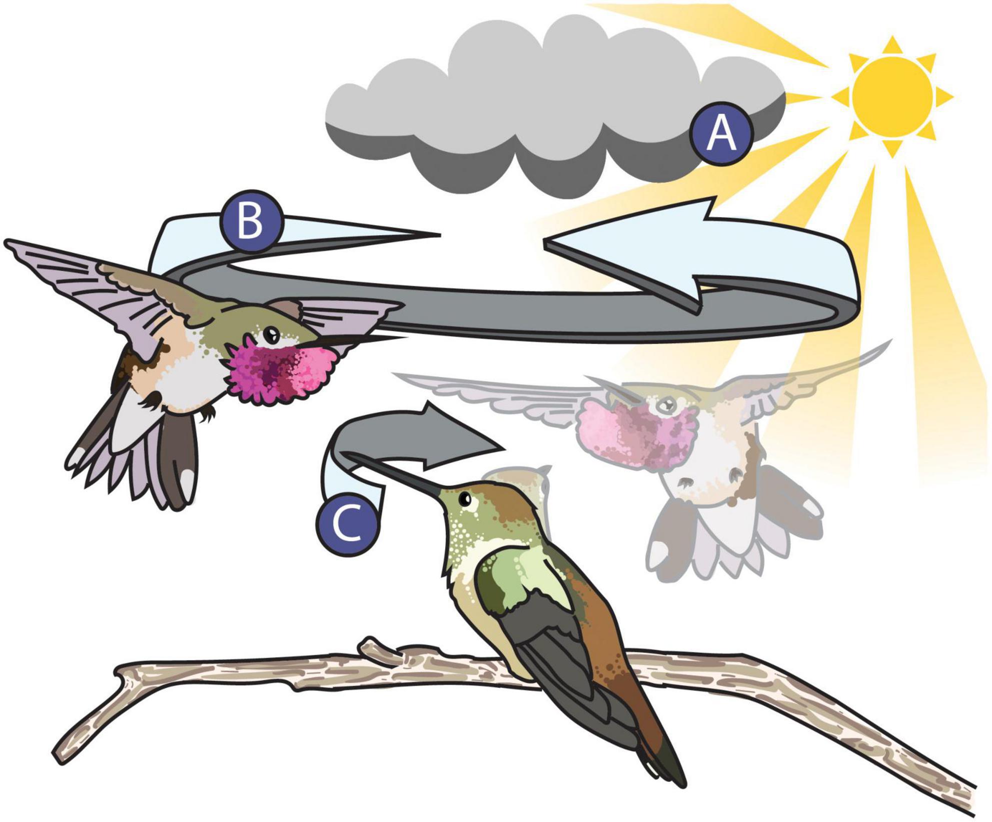
Figure 5. Illustration of the broad-tailed hummingbird shuttle display. The dynamic properties of the signaling environment (A), the signaler (B), and the receiver (C) can all alter the appearance of the male’s colorful display. (A) The signaling environment can influence the perception of animal signals. The male’s position relative to the position of the sun during his shuttle flight influences the perception or his iridescent magenta gorget. For example, the male’s gorget flashes more when he faces toward the sun but appears more consistent and UV in color when facing away from the sun (Simpson and McGraw, 2018). (B) The signaler—the male broad-tailed hummingbird—can alter the appearance of his gorget in two ways: by both manipulating his feathers into a disc to better direct it toward the female and by keeping a consistent orientation toward the female during his shuttle flight (Simpson and McGraw, 2018). (C) The receiver—the female broad-tailed hummingbird—might alter the perception of the signal by keeping the male in her field of view, which she accomplishes by moving her bill and head back and forth while watching the male. The extent to which this behavior influences the female’s perception of the male’s gorget during the shuttle display is unknown. A stock image from Pixabay (CC0 1.0) and photographs taken by ©Tom Walker and ©Wally Nussbaumer were used with their permission as reference material to illustrate this figure.

Equally, it is important to consider the position, distance, and direction of the receiver when studying dynamic visual signals. Receivers are usually active participants in signaling interactions and their movement can also influence the way colors are perceived. It is often difficult or impossible to position a camera in the location that best replicates a receiver’s view (Simpson and McGraw, 2018), but these specific geometric factors will influence an observer’s experience of a signal (Echeverri et al., 2021). An important advantage of 3D multispectral modeling techniques is the ability to intentionally position and animate cameras around a model during the rendering process. The introduction of unrestricted, user-defined camera views opens a variety of doors for animal coloration research by allowing for more accurate simulations of a receiver’s perspective (Bostwick et al., 2017). In Figure 5, the female broad-tailed hummingbird follows the male with her gaze during his shuttle courtship display. How well the female tracks the male during his display and how that impacts her perception of the shuttle is still unknown, but animated renders of multispectral models can help shed some light on how receiver motion might impact the appearance of colorful signals. With animated multispectral models, we can recreate the male’s movement in relation to the female and also animate virtual cameras to recreate the female’s viewing behavior in order to include the influence of receiver movement in a frame-by-frame analysis of male color. Such simulations would help address potential functional hypotheses for this conspicuous female behavior during the broad-tailed courtship display. For example, one hypothesis is that the female keeps the male in a certain area of her visual field to better view his display. Combined with existing tools that could be used to account for important visual properties like spatial resolution and acuity (AcuityView: Caves and Johnsen, 2018; QCPA: van den Berg et al., 2019), users can further tailor renders to match the receiver’s view.

Using animation, we can also simulate dynamism induced by the lighting environment and visual background. Generally, color is measured under consistent lighting conditions (Hutton et al., 2015) and in the absence of visual background, but signaling environments are often inherently heterogeneous and likely to influence the efficacy of visual signals (Hutton et al., 2015). In order to be conspicuous, signalers need to separate themselves from the physical environment during a signaling interaction. In the case of the broad-tailed hummingbird (Figure 5), the lighting environment can impact the appearance of his gorget during the shuttle display (Simpson and McGraw, 2018). The male’s gorget color increases in brightness, chroma, and red hue if the male is oriented toward the sun in his shuttle display. If the male is oriented away from the sun, his gorget appears more consistent in color and is more UV-shifted (Simpson and McGraw, 2018). With animated 3D multispectral modeling, we could simulate the visual background as well as the lighting environment during a male shuttle display and investigate if either strategy—(1) being flashier or (2) being more chromatically consistent—increases the visual saliency of the male against the natural background. Simulating dynamic signals in a virtual environment will be a valuable tool for understanding how animals signal effectively in a dynamic world.

While the current applications of this workflow involve virtual experiments completely in silico, a future application for animated 3D multispectral models could be in behavioral playback experiments. For example, it is not yet known what aspects of the male broad-tailed hummingbird shuttle display capture and hold female attention (Figure 5). These alerting components of the male’s signal are vital for effective communication of information during courtship (Endler, 1993; Endler and Mappes, 2017). 3D multispectral models could be used to investigate attentional mechanisms in dynamic colorful displays by creating virtual stimuli to present to live animal viewers, like female hummingbirds. Researchers could selectively modify different aspects of the male’s shuttle and measure the female’s response to determine which component (e.g., speed, gorget color/size/flashiness, sound, etc.), or combination of components, elicit the conspicuous viewing behavior performed by females during naturally occurring displays. One obstacle to this application is that current high-resolution LCD and LED screens do not emit UV light since most display screens are designed for human viewers—a problem that has been recognized for decades and remains unresolved (Cuthill et al., 2000). This is a real limitation for animals—like birds—with a wider range of wavelength sensitivity. However, technology is improving for creating bird-visible colors with LEDs and perhaps more sophisticated screens will be available in the future (Stoddard et al., 2020; Powell et al., 2021).

Conclusion

Recent developments in color quantification, 3D modeling, and animation mean that we are now better equipped to measure the colorful and often dynamic features of animal phenotypes. Here, we established a workflow for creating color-accurate UV/VIS 3D multispectral models of bird specimens with diffuse coloration—an important first step in generating new methods to quantify dynamic color. Our results suggest that the 3D multispectral models produced by this workflow contain color values comparable to those estimated using 2D multispectral imaging and spectrophotometry. We hope that this initial demonstration of our workflow will promote more work in developing 3D multispectral modeling pipelines. Generating color-accurate 3D multispectral models is an easy and effective way of producing data-rich digital renderings of animal specimens. Such models could transform the study and digitization of natural history museum specimens and inspire novel investigations of animal signaling in virtual worlds.

Data availability statement

The raw data supporting the conclusions of this article will be made available by the authors, without undue reservation.

Author contributions

AEM, BH, and MCS conceptualized the workflow, planned the study, revised, and approved the final manuscript. AEM and BH developed the workflow, collected, and analyzed the data. AEM produced figures and tables and wrote the first draft of the manuscript. All authors contributed to the article and approved the submitted version.

Funding

Funding to AEM was provided by the Princeton University. Funding to MCS was provided by Princeton University, a Packard Fellowship for Science and Engineering, and the National Science Foundation (Award #2029538).

Acknowledgments

We thank the Stoddard Lab for providing valuable feedback on the figures for this manuscript. We appreciate the valuable comments made by Jarome Ali, Klara Nordén, Monica Carlson, Sumudu Fernando, and Sarah Solie on drafts of the manuscript. We are grateful to the Macaulay Library at the Cornell Lab of Ornithology for sharing the video of the hooded pitta (ML201372881).

Conflict of interest

The authors declare that the research was conducted in the absence of any commercial or financial relationships that could be construed as a potential conflict of interest.

Publisher’s note

All claims expressed in this article are solely those of the authors and do not necessarily represent those of their affiliated organizations, or those of the publisher, the editors and the reviewers. Any product that may be evaluated in this article, or claim that may be made by its manufacturer, is not guaranteed or endorsed by the publisher.

Supplementary material

The Supplementary Material for this article can be found online at: https://www.frontiersin.org/articles/10.3389/fevo.2022.983369/full#supplementary-material

Footnotes

1. ^ https://github.com/audreyem/ColorInMotion
2. ^ http://digicamcontrol.com/

References

Agisoft Metashape User Manual, (2022) Agisoft Metashape User Manual - Professional Edition, Version 1.8.

Google Scholar

Akkaynak, D., Treibitz, T., Xiao, B., Gürkan, U. A., Allen, J. J., Demirci, U., et al. (2014). Use of commercial off-the-shelf digital cameras for scientific data acquisition and scene-specific color calibration. J. Opt. Soc. Am. A 31:312. doi: 10.1364/JOSAA.31.000312

PubMed Abstract | CrossRef Full Text | Google Scholar

Allen, W. L., Baddeley, R., Cuthill, I. C., and Scott-Samuel, N. E. (2012). A Quantitative test of the predicted relationship between countershading and lighting environment. Am. Nat. 180, 762–776. doi: 10.1086/668011

PubMed Abstract | CrossRef Full Text | Google Scholar

Bishop, P. J., Cuff, A. R., and Hutchinson, J. R. (2021). How to build a dinosaur: Musculoskeletal modeling and simulation of locomotor biomechanics in extinct animals. Paleobiology 47, 1–38. doi: 10.1017/pab.2020.46

CrossRef Full Text | Google Scholar

Bostwick, K. S., Harvey, T. A., and Scholes, E. I. I. I. (2017). “Leveraging diverse specimen types to integrate behavior and morphophology,” in The extended specimen: Emerging frontiers in collection-based ornithological research, ed. M. S. Webster (Boca Raton, FL: CRC Press).

Google Scholar

Bot, J. A., and Irschick, D. J. (2019). “Using 3D photogrammetry to create openacess models of live animal: 2D and 3D software solutions,” in 3D/VR in the academic library: Emerging practices and trends, eds J. Grayburn, Z. L. Katz, K. G. Davis, and V. I. Orlati (Alexandria, VA: Council on Library and Information Resources).

Google Scholar

Brown, D. (2022). A workflow and tips for creating 3D models of amphibians and reptiles using photogrammetry. Herpetol. Rev. 53, 34–38.

Google Scholar

Burns, K. J., McGraw, K. J., Shultz, A. J., Stoddard, M. C., and Thomas, D. B. (2017). “Advanced methods for studying pigments and coloration using avian specimens 1, 2,” in The extended specimen: Emerging frontiers in collections-based ornithological research, ed. M. S. Webster (Boca Raton, FL: CRC Press).

Google Scholar

Caves, E. M., and Johnsen, S. (2018). AcuityView: An R package for portraying the effects of visual acuity on scenes observed by an animal. Methods Ecol. Evol. 9, 793–797. doi: 10.1111/2041-210X.12911

CrossRef Full Text | Google Scholar

Chiao, C.-C., and Cronin, T. W. (2002). Hyperspecrtral imaging for color vision research. Recent Res. Dev. Optics 2, 465–482.

Google Scholar

Chiari, Y., Wang, B., Rushmeier, H., and Caccone, A. (2008). Using digital images to reconstruct three-dimensional biological forms: a new tool for morphological studies. Biol. J. Linnean Soc. 95, 425–436. doi: 10.1111/j.1095-8312.2008.01055.x

CrossRef Full Text | Google Scholar

Chouinard-Thuly, L., Gierszewski, S., Rosenthal, G. G., Reader, S. M., Rieucau, G., Woo, K. L., et al. (2017). Technical and conceptual considerations for using animated stimuli in studies of animal behavior. Curr. Zool. 63, 5–19. doi: 10.1093/cz/zow104

PubMed Abstract | CrossRef Full Text | Google Scholar

Cooney, C. R., He, Y., Varley, Z. K., Nouri, L. O., Moody, C. J. A., Jardine, M. D., et al. (2022). Latitudinal gradients in avian colourfulness. Nat. Ecol. Evol. 6, 622–629. doi: 10.1038/s41559-022-01714-1

PubMed Abstract | CrossRef Full Text | Google Scholar

Corcoran, A. J., Schirmacher, M. R., Black, E., and Hedrick, T. L. (2021). ThruTracker: Open-source software for 2-d and 3-d animal video tracking. bioRxiv [Preprint] doi: 10.1101/2021.05.12.443854

CrossRef Full Text | Google Scholar

Cuthill, I. C., Allen, W. L., Arbuckle, K., Caspers, B., Chaplin, G., Hauber, M. E., et al. (2017). The biology of color. Science 357:eaan0221. doi: 10.1126/science.aan0221

PubMed Abstract | CrossRef Full Text | Google Scholar

Cuthill, I. C., Hart, N. S., Partridge, J. C., Bennett, A. T. D., Hunt, S., and Church, S. C. (2000). Avian colour vision and avian video playback experiments. Acta Ethol. 3, 29–37. doi: 10.1007/s102110000027

CrossRef Full Text | Google Scholar

Delhey, K., Delhey, V., Kempenaers, B., and Peters, A. (2015). A practical framework to analyze variation in animal colors using visual models. Behav. Ecol. 26, 367–375. doi: 10.1093/beheco/aru198

CrossRef Full Text | Google Scholar

Dell, A. I., Bender, J. A., Branson, K., Couzin, I. D., de Polavieja, G. G., Noldus, L. P. J. J., et al. (2014). Automated image-based tracking and its application in ecology. Trends Ecol. Evol. 29, 417–428. doi: 10.1016/j.tree.2014.05.004

PubMed Abstract | CrossRef Full Text | Google Scholar

DeLorenzo, L., Linden, A. V., Bergmann, P. J., Wagner, G. P., Siler, C. D., and Irschick, D. J. (2020). Using 3D-digital photogrammetry to examine scaling of the body axis in burrowing skinks. J. Morphol. 281, 1382–1390. doi: 10.1002/jmor.21253

PubMed Abstract | CrossRef Full Text | Google Scholar

Echeverri, S. A., Miller, A. E., Chen, J., McQueen, E. W., Plakke, M., Spicer, M., et al. (2021). How signaling geometry shapes the efficacy and evolution of animal communication systems. Int. Comp. Biol. 61, 787–813. doi: 10.1093/icb/icab090

PubMed Abstract | CrossRef Full Text | Google Scholar

Endler, J. A. (1993). Some general comments on the evolution and design of animal communication systems. Philos. Trans. Biol. Sci. 340, 215–225. doi: 10.1098/rstb.1993.0060

PubMed Abstract | CrossRef Full Text | Google Scholar

Endler, J. A., and Mappes, J. (2017). The current and future state of animal coloration research. Phil. Trans. R. Soc. B 372:20160352. doi: 10.1098/rstb.2016.0352

PubMed Abstract | CrossRef Full Text | Google Scholar

Endler, J. A., and Mielke, P. W. (2005). Comparing entire colour patterns as birds see them. Biol. J. Linnean Soc. 86, 405–431. doi: 10.1111/j.1095-8312.2005.00540.x

CrossRef Full Text | Google Scholar

Fangbemi, A. S., Lu, Y. F., Xu, M. Y., Luo, X. W., Rolland, A., and Raissi, C. (2020). ZooBuilder: 2D and 3D pose estimation for quadrupeds using synthetic data. arXiv [Preprint]. arXiv: 2009.05389.

Google Scholar

Fortuny, J., Marcé-Nogué, J., Heiss, E., Sanchez, M., Gil, L., and Galobart, À (2015). 3D bite modeling and feeding mechanics of the largest living amphibian, the chinese giant salamander Andrias davidianus (Amphibia:Urodela). PLoS One 10:e0121885. doi: 10.1371/journal.pone.0121885

PubMed Abstract | CrossRef Full Text | Google Scholar

Frith, D. W., and Frith, C. B. (1988). Courtship display and mating of the superb bird of paradise lophorina superb. EMU - Austral Ornithol. 88, 183–188. doi: 10.1071/MU9880183

CrossRef Full Text | Google Scholar

Gatesy, S. M., Baier, D. B., Jenkins, F. A., and Dial, K. P. (2010). Scientific rotoscoping: a morphology-based method of 3-D motion analysis and visualization. J. Exp. Zool. Part A: Ecol. Genetics Physiol. 313A, 244–261. doi: 10.1002/jez.588

PubMed Abstract | CrossRef Full Text | Google Scholar

Gómez, J., Ramo, C., Troscianko, J., Stevens, M., Castro, M., Pérez-Hurtado, A., et al. (2018). Individual egg camouflage is influenced by microhabitat selection and use of nest materials in ground-nesting birds. Behav. Ecol. Sociobiol. 72:142. doi: 10.1007/s00265-018-2558-7

CrossRef Full Text | Google Scholar

Graving, J. M., Chae, D., Naik, H., Li, L., Koger, B., Costelloe, B. R., et al. (2019). DeepPoseKit, a software toolkit for fast and robust animal pose estimation using deep learning. eLife 8:e47994. doi: 10.7554/eLife.47994

PubMed Abstract | CrossRef Full Text | Google Scholar

Hart, N. S., and Hunt, D. M. (2007). Avian visual pigments: characteristics. spectral tuning, and evolution. Am. Nat. 169, S7–S26. doi: 10.1086/510141

PubMed Abstract | CrossRef Full Text | Google Scholar

Hart, N. S., Partridge, J. C., Cuthill, I. C., and Bennett, A. T. D. (2000). Visual pigments, oil droplets, ocular media and cone photoreceptor distribution in two species of passerine bird: the blue tit (Parus caeruleus L.) and the blackbird (Turdus merula L.). J. Comp. Physiol. Sensory Neural Behav. Physiol. 186, 375–387. doi: 10.1007/s003590050437

PubMed Abstract | CrossRef Full Text | Google Scholar

Harvey, T. A., Bostwick, K. S., and Marschner, S. (2013). Measuring spatially- and directionally-varying light scattering from biological material. JoVE (J. Vis. Exp.) 75:e50254. doi: 10.3791/50254

PubMed Abstract | CrossRef Full Text | Google Scholar

Hutton, P., Seymoure, B. M., McGraw, K. J., Ligon, R. A., and Simpson, R. K. (2015). Dynamic color communication. Curr. Opin. Behav. Sci. 6, 41–49. doi: 10.1016/j.cobeha.2015.08.007

CrossRef Full Text | Google Scholar

Irschick, D. J., Corriveau, Z., Mayhan, T., Siler, C., Mandica, M., Gamble, T., et al. (2020). Devices and methods for rapid 3D photo-capture and photogrammetry of small reptiles and amphibians in the laboratory and the field. Herpetol. Rev. 51, 716–725.

Google Scholar

Irschick, D. J., Martin, J., Siebert, U., Kristensen, J. H., Madsen, P. T., and Christiansen, F. (2021). Creation of accurate 3D models of harbor porpoises (Phocoena phocoena) using 3D photogrammetry. Mar. Mammal Sci. 37, 482–491. doi: 10.1111/mms.12759

CrossRef Full Text | Google Scholar

Iskandar, J.-P., Eliason, C. M., Astrop, T., Igic, B., Maia, R., and Shawkey, M. D. (2016). Morphological basis of glossy red plumage colours. Biol. J. Linnean Soc. 119, 477–487. doi: 10.1111/bij.12810

CrossRef Full Text | Google Scholar

Jackson, B. E., Evangelista, D. J., Ray, D. D., and Hedrick, T. L. (2016). 3D for the people: Multi-camera motion capture in the field with consumer-grade cameras and open source software. Biol. Open 5, 1334–1342. doi: 10.1242/bio.018713

PubMed Abstract | CrossRef Full Text | Google Scholar

Jakob, W., Tarini, M., Panozzo, D., and Sorkine-Hornung, O. (2015). Instant field-aligned meshes. ACM Trans. Graph. 34, 1–15. doi: 10.1145/2816795.2818078

CrossRef Full Text | Google Scholar

Kim, M. H., Harvey, T. A., Kittle, D. S., Rushmeier, H., Dorsey, J., Prum, R. O., et al. (2012). “3D imaging spectroscopy for measuring hyperspectral patterns on solid objects,” in Proceedings of the ACM Transactions on Graphics, (New York, NY). doi: 10.1145/2185520.2185534

CrossRef Full Text | Google Scholar

Künzler, R., and Bakker, T. C. M. (1998). Computer animations as a tool in the study of mating preferences. Behaviour 135, 1137–1159.

Google Scholar

Leavesley, S., Ahmed, W., Bayraktar, B., Rajwa, B., Strugis, J., and Robinson, J. P. (2005). Multispectral imaging analysis: spectral deconvolution and applications in biology. Proc. SPIE 5699:121. doi: 10.1117/12.598065

CrossRef Full Text | Google Scholar

Maia, R., Gruson, H., Endler, J. A., and White, T. E. (2019). pavo 2: new tools for the spectral and spatial analysis of colour in R. Methods Ecol. Evol. 10, 1097–1107. doi: 10.1111/2041-210X.13174

CrossRef Full Text | Google Scholar

Maia, R., and White, T. E. (2018). Comparing colors using visual models. Behav. Ecol. 29, 649–659. doi: 10.1093/beheco/ary017

CrossRef Full Text | Google Scholar

Mäthger, L. M., Denton, E. J., Marshall, N. J., and Hanlon, R. T. (2009). Mechanisms and behavioural functions of structural coloration in cephalopods. J. R. Soc. Interface 6, S149–S163. doi: 10.1098/rsif.2008.0366.focus

PubMed Abstract | CrossRef Full Text | Google Scholar

McCoy, D. E., Shultz, A. J., Vidoudez, C., van der Heide, E., Dall, J. E., Trauger, S. A., et al. (2021). Microstructures amplify carotenoid plumage signals in tanagers. Sci. Rep. 11:8582. doi: 10.1038/s41598-021-88106-w

PubMed Abstract | CrossRef Full Text | Google Scholar

Medina, J. J., Maley, J. M., Sannapareddy, S., Medina, N. N., Gilman, C. M., and McCormack, J. E. (2020). A rapid and cost-effective pipeline for digitization of museum specimens with 3D photogrammetry. PLoS One 15:e0236417. doi: 10.1371/journal.pone.0236417

PubMed Abstract | CrossRef Full Text | Google Scholar

Miles, M. C., and Fuxjager, M. J. (2019). Phenotypic diversity arises from secondary signal loss in the elaborate visual displays of toucans and barbets. Am. Nat. 194, 152–167. doi: 10.1086/704088

PubMed Abstract | CrossRef Full Text | Google Scholar

Müller, K., Smielik, I., Hütwohl, J.-M., Gierszewski, S., Witte, K., and Kuhnert, K.-D. (2017). The virtual lover: Variable and easily guided 3D fish animations as an innovative tool in mate-choice experiments with sailfin mollies-I. Design and implementation. Curr. Zool. 63, 55–64. doi: 10.1093/cz/zow106

PubMed Abstract | CrossRef Full Text | Google Scholar

Mumme, R. L. (2014). White tail spots and tail-flicking behavior enhance foraging performance in the Hooded Warbler. Auk 131, 141–149. doi: 10.1642/AUK-13-199.1

PubMed Abstract | CrossRef Full Text | Google Scholar

Nath, T., Mathis, A., Chen, A. C., Patel, A., Bethge, M., and Mathis, M. W. (2019). Using DeepLabCut for 3D markerless pose estimation across species and behaviors. Nat. Protoc. 14, 2152–2176. doi: 10.1038/s41596-019-0176-0

PubMed Abstract | CrossRef Full Text | Google Scholar

Negro, J. J., Sarasola, J. H., Fariñas, F., and Zorrilla, I. (2006). Function and occurrence of facial flushing in birds. Comp. Biochem. Physiol. Part A: Mol. Int. Physiol. 143, 78–84. doi: 10.1016/j.cbpa.2005.10.028

PubMed Abstract | CrossRef Full Text | Google Scholar

Nguyen, C. V., Lovell, D. R., Adcock, M., and Salle, J. L. (2014). Capturing natural-colour 3D models of insects for species discovery and diagnostics. PLoS One 9:e94346. doi: 10.1371/journal.pone.0094346

PubMed Abstract | CrossRef Full Text | Google Scholar

Olsson, P., Lind, O., and Kelber, A. (2018). Chromatic and achromatic vision: parameter choice and limitations for reliable model predictions. Behav. Ecol. 29, 273–282. doi: 10.1093/beheco/arx133

CrossRef Full Text | Google Scholar

Osorio, D., and Vorobyev, M. (2005). Photoreceptor sectral sensitivities in terrestrial animals: adaptations for luminance and colour vision. Proc. R. Soc. B. 272, 1745–1752. doi: 10.1098/rspb.2005.3156

PubMed Abstract | CrossRef Full Text | Google Scholar

Pike, T. W. (2011). Using digital cameras to investigate animal colouration: estimating sensor sensitivity functions. Behav. Ecol. Sociobiol. 65, 849–858. doi: 10.1007/s00265-010-1097-7

CrossRef Full Text | Google Scholar

Powell, S. B., Mitchell, L. J., Phelan, A. M., Cortesi, F., Marshall, J., and Cheney, K. L. (2021). A five-channel LED display to investigate UV perception. Methods Ecol. Evol. 12, 602–607. doi: 10.1111/2041-210X.13555

CrossRef Full Text | Google Scholar

Price-Waldman, R., and Stoddard, M. C. (2021). Avian coloration genetics: recent advances and emerging questions. J. Heredity 112, 395–416. doi: 10.1093/jhered/esab015

PubMed Abstract | CrossRef Full Text | Google Scholar

R Core Team (2017). R: A Language and Environment for Statistical Computing. Vienna: R Foundation for Statistical Computing.

Google Scholar

Renoult, J. P., Kelber, A., and Schaefer, H. M. (2017). Colour spaces in ecology and evolutionary biology. Biol. Rev. 92, 292–315. doi: 10.1111/brv.12230

PubMed Abstract | CrossRef Full Text | Google Scholar

Rosenthal, G. G. (2007). Spatiotemporal dimensions of visual signals in animal communication. Annu. Rev. Ecol. Evol. Syst. 38, 155–178. doi: 10.1146/annurev.ecolsys.38.091206.095745

CrossRef Full Text | Google Scholar

Rowland, H. M. (2009). From Abbott Thayer to the present day: What have we learned about the function of countershading? Philos. Trans. R. Soc. B 364, 519–527. doi: 10.1098/rstb.2008.0261

PubMed Abstract | CrossRef Full Text | Google Scholar

Schneider, C. A., Rasband, W. S., and Eliceiri, K. W. (2012). NIH Image to ImageJ: 25 years of image analysis. Nat. Methods 9, 671–675. doi: 10.1038/nmeth.2089

PubMed Abstract | CrossRef Full Text | Google Scholar

Siddiqi, A., Cronin, T. W., Loew, E. R., Vorobyev, M., and Summers, K. (2004). Interspecific and intraspecific views of color signals in the strawberry poison frog Dendrobates pumilio. J. Exp. Biol. 207, 2471–2485. doi: 10.1242/jeb.01047

PubMed Abstract | CrossRef Full Text | Google Scholar

Silvasti, S. A., Valkonen, J. K., and Nokelainen, O. (2021). Behavioural thresholds of blue tit colour vision and the effect of background chromatic complexity. Vis. Res. 182, 46–57. doi: 10.1016/j.visres.2020.11.013

PubMed Abstract | CrossRef Full Text | Google Scholar

Simpson, R. K., and McGraw, K. J. (2018). Two ways to display: male hummingbirds show different color-display tactics based on sun orientation. Behav. Ecol. 29, 637–648. doi: 10.1093/beheco/ary016

CrossRef Full Text | Google Scholar

Smith, T., and Guild, J. (1931). The C.I.E. colorimetric standards and their use. Trans. Opt. Soc. 33, 73–134. doi: 10.1088/1475-4878/33/3/301

CrossRef Full Text | Google Scholar

Stavenga, D. G., Leertouwer, H. L., Marshall, N. J., and Osorio, D. (2011). Dramatic colour changes in a bird of paradise caused by uniquely structured breast feather barbules. Proc. R. Soc. B: Biol. Sci. 278, 2098–2104. doi: 10.1098/rspb.2010.2293

PubMed Abstract | CrossRef Full Text | Google Scholar

Stevens, M., Párraga, C. A., Cuthill, I. C., Partridge, J. C., and Troscianko, T. S. (2007). Using digital photography to study animal coloration. Biol. J. Linnean Soc. 90, 211–237. doi: 10.1111/j.1095-8312.2007.00725.x

CrossRef Full Text | Google Scholar

Stoddard, M. C., and Prum, R. O. (2008). Evolution of avian plumage color in a tetrahedral color space: a phylogenetic analysis of new world buntings. Am. Nat. 171, 755–776. doi: 10.1086/587526

PubMed Abstract | CrossRef Full Text | Google Scholar

Stoddard, M. C., Eyster, H. N., Hogan, B. G., Morris, D. H., Soucy, E. R., and Inouye, D. W. (2020). Wild hummingbirds discriminate nonspectral colors. Proc. Natl. Acad. Sci. U.S.A. 117, 15112–15122. doi: 10.1073/pnas.1919377117

PubMed Abstract | CrossRef Full Text | Google Scholar

Sun, Y. (2006). Rendering biological iridescences with RGB-based renderers. ACM Trans. Graphics 25, 100–129.

Google Scholar

Troscianko, J., and Stevens, M. (2015). Image calibration and analysis toolbox - a free software suite for objectively measuring reflectance, colour and pattern. Methods Ecol. Evol. 6, 1320–1331. doi: 10.1111/2041-210X.12439

PubMed Abstract | CrossRef Full Text | Google Scholar

van den Berg, C. P., Troscianko, J., Endler, J. A., Marshall, N. J., and Cheney, K. L. (2019). Quantitative Colour Pattern Analysis (QCPA): a comprehensive framework for the analysis of colour patterns in nature. Methods Ecol. Evol. 11, 316–332.

Google Scholar

Veneziano, A., Landi, F., and Profico, A. (2018). Surface smoothing, decimation, and their effects on 3D biological specimens. Am. J. Phys. Anthropol. 166, 473–480. doi: 10.1002/ajpa.23431

PubMed Abstract | CrossRef Full Text | Google Scholar

Vinther, J., Nicholls, R., Lautenschlager, S., Pittman, M., Kaye, T. G., Rayfield, E., et al. (2016). 3D camouflage in an ornithischian dinosaur. Curr. Biol. 26, 2456–2462. doi: 10.1016/j.cub.2016.06.065

PubMed Abstract | CrossRef Full Text | Google Scholar

Vorobyev, M., and Osorio, D. (1998). Receptor noise as a determinant of colour thresholds. Proc. R. Soc. Lond. B 265, 351–358. doi: 10.1098/rspb.1998.0302

PubMed Abstract | CrossRef Full Text | Google Scholar

Webster, M. S. (2017). “The extended specimen,” in The extended specimen: Emerging frontiers in collections-based ornithological research, ed. M. S. Webster (Boca Raton, FL: CRC Press).

Google Scholar

Westoby, M., Brasington, J., Glasser, N., Hambrey, M., and Reynolds, J. (2012). Structure-from-Motion photogrammetry: a novel, low-cost tool for geomorphological applications. Geomorphology 179, 300–314.

Google Scholar

White, T., Maia, R., Endler, J., Eliason, C., and Bitton, P.-P. (2021). pavo: Perceptual Analysis, Visualization and Organization of Spectral Colour Data. Version 2.7.1. CRAN.

Google Scholar

Witte, K., Gierszewski, S., Chouinard-Thuly, L., and Guest Editors. (2017). Virtual is the new reality. Curr. Zool. 63, 1–4. doi: 10.1093/cz/zow119

PubMed Abstract | CrossRef Full Text | Google Scholar

Woo, K. L., Rieucau, G., and Burke, D. (2017). Computer-animated stimuli to measure motion sensitivity: Constraints on signal design in the Jacky dragon. Curr. Zool. 63, 75–84. doi: 10.1093/cz/zow074

PubMed Abstract | CrossRef Full Text | Google Scholar

Zimova, M., Hackländer, K., Good, J. M., Melo-Ferreira, J., Alves, P. C., and Mills, L. S. (2018). Function and underlying mechanisms of seasonal colour moulting in mammals and birds: what keeps them changing in a warming world? Biol. Rev. 93, 1478–1498. doi: 10.1111/brv.12405

PubMed Abstract | CrossRef Full Text | Google Scholar

Zuffi, S., Kanazawa, A., Jacobs, D. W., and Black, M. J. (2017). “3D menagerie: Modeling the 3d shape and pose of animals,” in Proceedings of the 2017 IEEE conference on computer vision and pattern recognition (CVPR), Honolulu, HI, 5524–5532. doi: 10.1109/CVPR.2017.586

CrossRef Full Text | Google Scholar

Zylinski, S., Osorio, D., and Shohet, A. J. (2009). Cuttlefish camouflage: context-dependent body pattern use during motion. Proc. R. Soc. B: Biol. Sci. 276, 3963–3969. doi: 10.1098/rspb.2009.1083

PubMed Abstract | CrossRef Full Text | Google Scholar