How asymmetric mating patterns affect the rate of neutral genetic substitution

1. Introduction

In a well-mixed population, for a genetic locus experiencing rare, neutral mutation, the expected rate of genetic substitution per generation, K, is equal to the probability of mutation per birth, u. This result, first demonstrated by Kimura (1968), can be derived simply as follows: the expected number of substitutions per generation is K = nuρ, where n is the number of alleles (equal to the population size N for haploids, or 2N for diploids), and ρ is the probability that a neutral mutation will become fixed. In a well-mixed population, this neutral fixation probability is ρ = 1/n, leading to K = u. This result underpins the idea of the “molecular clock”—that substitutions at neutral loci can be used to estimate the timing of events in evolutionary history (Ayala, 1997; Bromham and Penny, 2003; Kumar, 2005). The K = u result also extends to spatially structured populations with a high degree of symmetry (Maruyama, 1970; Nagylaki, 1982).

However, Allen et al. (2015) showed that asymmetries in the spatial structure can lead to either ρ > 1/n or ρ < 1/n, thereby altering the rate K of substitutions per generation. This occurs because both the fixation probability and the rate of replacement can vary across spatial locations. Sites that are frequently replaced have a higher rate of new mutations. If a frequently-replaced site is favorable to mutant fixation, this can increase the average fixation probability ρ above 1/n. In this way, asymmetric spatial structure can either speed up or slow down the neutral substitution rate K.

The results of Allen et al. (2015) were derived for haploid, spatially structured populations. Here we show that the same phenomenon can arise for diploid populations with asymmetric mating patterns. We present a general method for calculating the neutral fixation probability ρ under arbitrary mating pattern. This fixation probability can be compared to the corresponding value of ${\rho }_{\text{WM}}=\frac{1}{2N}$ for a well-mixed population of N individuals.

We apply this framework to two hypothetical scenarios: a randomly mating population with uneven sex ratio, and a population with reproductive skew in one sex. In each case we show that asymmetries in the mating pattern and replacement rate can lead to $\rho >\frac{1}{2N}$ or $\rho <\frac{1}{2N}$, accelerating or slowing the rate K of neutral genetic substitution. Specifically, we identify two circumstances in which the neutral substitution rate is altered: (1) the sex ratio is unequal at birth and there is differential mortality between the sexes, or (2) there is reproductive skew in one sex, and differential mortality between high-reproducing and low-reproducing individuals. The first scenario may arise in reptiles with temperature-dependent sex determination (Ferguson and Joanen, 1982; Ewert and Nelson, 1991), while the second may apply to a variety of birds (Wiley, 1973; Petrie et al., 1991; Höglund and Alatalo, 1995; Magrath et al., 2004), mammals (Boesch et al., 2006; Raihani and Clutton-Brock, 2010; Sherman et al., 2017; Higham et al., 2021), and insects (Adams and Atkinson, 2008; Shimoji and Dobata, 2022).

2. Modeling framework

We begin by summarizing the mathematical framework from which our results are derived. A formal description of this framework is given in the Supplementary material.

2.1. Mating and replacement

We consider a diploid population of fixed size N, which can be monoecious (one sex) or dioecious (two sexes). The individuals are indexed I = 1, …, N. Depending on the model in question, each index I may also designate other relevant information, such as the sex and/or spatial location of individual I.

Each time-step, some subset of individuals are replaced by new offspring. Each new offspring has two parents (which may be the same individual in the case of self-mating). The set of individuals to be replaced, as well as the parents of each new offspring, are sampled from a fixed probability distribution. This probability distribution can be chosen arbitrarily, subject only to the requirement that it be possible for a mutant allele to spread throughout the population. In this way, our framework can incorporate a wide variety of spatial structures and mating patterns, with no assumption of symmetry or uniformity. This level of generality is achieved using an abstract mathematical representation of population structure, which was developed in previous works (Allen and Tarnita, 2014; Allen et al., 2015; Allen and McAvoy, 2019) and is further extended in the Supplementary material to include arbitrary mating patterns.

The key quantities describing any particular model within this framework are the mating and replacement rates $E_{IJ}^K$, where the indices I, J, and K run from 1 to N, representing individuals in the population (Figure 1). For I ≠ J, $E_{IJ}^K$ is equal to the marginal probability that, in a given time-step, individual K is replaced by the offspring of I and J. The subscript indices in $E_{IJ}^K$ are understood as an unordered pair, meaning that $E_{IJ}^K$ and $E_{JI}^K$ both refer to the same marginal probability. In the case of self-mating, $E_{II}^K$ is set equal to twice the marginal probability that K is replaced by the self-mated offspring of I (the factor of two accounts for the doubled chance to spread one's alleles under self-mating). These $E_{IJ}^K$ quantities take into account the population's spatial structure and dispersal patterns as well as its mating pattern.

FIGURE 1

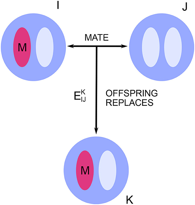
Figure 1. Neutral drift in a diploid population. In each time-step, some individuals are replaced by the offspring of others. These mating and replacement events are sampled from a fixed probability distribution, which captures all effects of spatial structure and mating pattern. The key quantities are the marginal probabilities $E_{IJ}^K$ that, in a given time-step, individual K is replaced by the offspring of I and J. There are two allele types, mutant and resident. Each new offspring inherits alleles from its parents according to Mendelian inheritance.

For each individual I = 1, …, N, we define the death rate D_I as the marginal probability that I is replaced, and the birth rate B_I as half the expected offspring number of I. In terms of the mating and replacement rates $E_{IJ}^K$, the birth and death rates are given by

$\begin{array}{ll}{B}_I=\frac{1}{2}{\displaystyle \sum _{J,K}}{E}_{IJ}^K,& (1)\end{array}$

$\begin{array}{ll}{D}_I=\frac{1}{2}{\displaystyle \sum _{J,K}}{E}_{JK}^I.& (2)\end{array}$

The factors of $\frac{1}{2}$ in B_I and D_I arise for different reasons: for D_I a $\frac{1}{2}$ is needed to avoid double-counting in the J and K indices, while for B_I the $\frac{1}{2}$ represents the chance of transmitting a particular allele under Mendelian inheritance. We also define the overall rate of turnover, B, as

$\begin{array}{ll}B={\displaystyle \sum _{I=1}^N}{B}_I={\displaystyle \sum _{I=1}^N}{D}_I=\frac{1}{2}{\displaystyle \sum _{I,J,K}}{E}_{IJ}^K.& (3)\end{array}$

2.2. Alleles and states

Within the population we consider two allele variants: a resident allele R, and a neutral mutant allele M. Each new offspring inherit alleles from its parents according to Mendelian inheritance. We assume there is no recurring mutation, so that, over time, either the mutant or the resident allele will become fixed in the population.

The state of the population at any given time can be specified by identifying the genotype (MM, MR, or RR) of each individual I = 1, …, N. Since the mutant allele is neutral, the mating and replacement rates $E_{IJ}^K$ do not depend on the current population state. The overall process of neutral drift is represented as a Markov chain on the set of population states (see the Supplementary material for details).

3. Fixation probability

Over time, the neutral drift process will ultimately converge to a state where either only mutant or only resident alleles are present. We are interested in the fixation probability of the mutant type; that is, the probability of reaching the all-mutant state when starting from a state with only a single mutant allele.

3.1. Deriving fixation probability

Let ρ_I denote the probability that the all-mutant state is reached, when starting from a state with a single mutant allele copy in individual I. The neutral fixation probability ρ_I can also be understood as the reproductive value of individual I (Taylor, 1990; Lehmann, 2014; Maciejewski, 2014; Allen and McAvoy, 2019), since it quantifies I's contribution to the future gene pool.

In the Supplementary material we derive the recurrence equation for the reproductive values ρ_I:

$\begin{array}{ll}{\rho }_I=(1-D_I){\rho }_I+\frac{1}{2}{\displaystyle \sum _{J,K}}{E}_{IJ}^K{\rho }_K.& (4)\end{array}$

The two terms on the right-hand side correspond to survival and transmission, respectively, of a mutant allele. The $\frac{1}{2}$ in the second term reflects the chance of transmission to offspring under Mendelian inheritance. These probabilities of survival or transmission are multiplied by the reproductive values, ρ_I or ρ_K, of this allele and its copies in the next time-step.

We can write Eq. (4) in simpler form as

$\begin{array}{ll}{D}_I{\rho }_I=\frac{1}{2}{\displaystyle \sum _{J,K}}{E}_{IJ}^K{\rho }_K.& (5)\end{array}$

In order to solve for the fixation probabilities, we also require the equation

$\begin{array}{ll}2{\displaystyle \sum _{I=1}^N}{\rho }_I=1.& (6)\end{array}$

Equation (6) represents the fact that exactly one of the 2N initial alleles will ultimately spread its descendants throughout the population, and the probability of this occurring for an allele in individual I is ρ_I.

Together, Eqs. (5) and (6) form a system of equations that uniquely determine ρ_I for each I = 1, …, N. Although this system involves N + 1 equations, one case of Eq. (5) is always redundant and can be eliminated. If the population can be subdivided into classes (by sex, spatial location, etc.) such that individuals in a given class are interchangeable, only one equation per class is needed. This will be the case in the examples we explore later.

To determine the overall fixation probability, we must take into account where mutations arise. Supposing that mutations occur with constant probability per birth, the likelihood of a new mutant allele arising at individual I is proportional to the turnover rate D_I. We therefore suppose the initial mutation has probability D_I/B of arising within individual I, for each I = 1, …, N. This leads to an overall fixation probability of

$\begin{array}{ll}\rho =\frac{1}{B}{\displaystyle \sum _{I=1}^N}{D}_I{\rho }_I.& (7)\end{array}$

3.2. Comparing to well-mixed population

A well-mixed, monoecious (one sex) population with uniform random mating has the same value of $E_{IJ}^K$ for each triple I, J, K. In this case, Eqs. (1)–(7) yield an overall fixation probability of ${\rho }_{\text{WM}}=\frac{1}{2N}$, which we take as our baseline value. We are interested in when and how ρ can differ from ρ_WM, in populations for which the replacement rates $E_{IJ}^K$ take on non-uniform values due to asymmetric mating patterns and/or spatial structure.

We first note that, by combining Eqs. (3), (6), and (7), we can write

$\begin{array}{l}\rho -{\rho }_{\text{WM}}=\frac{N}{B}\left(\frac{1}{N}{\displaystyle \sum _{I=1}^N}{D}_I{\rho }_I-\left(\frac{1}{N}{\displaystyle \sum _{I=1}^N}{D}_I\right)\left(\frac{1}{N}{\displaystyle \sum _{I=1}^N}{\rho }_I\right)\right)\\ =\frac{N}{B}{Cov}_I\left[D,\rho \right].& (8)\end{array}$

Above, Cov_I[D, ρ] is the population covariance of D_I with ρ_I over I = 1, …, N, which is equal by definition to the quantity inside parentheses in the second expression. It follows that ρ > ρ_WM if D_I and ρ_I are positively correlated, ρ < ρ_WM if D_I and ρ_I are negatively correlated, and ρ = ρ_WM if they are uncorrelated.

In particular, we will have ρ = ρ_WM if either D_I or ρ_I are constant over individuals. These two cases correspond to Results 1 and 2 of Allen et al. (2015), which we extend here to diploid populations. First, Eq. (8) immediately leads to

Result 1. If D_I constant over all I = 1, …, N, then $\rho ={\rho }_{\text{WM}}(=\frac{1}{2N})$.

That is, if mortality is constant across individuals—mathematically, if $\sum _{I,J}{E}_{IJ}^K$ is uniform over K—the rate of neutral substitution is unchanged from the baseline rate.

The second case, constant ρ_I, turns out to be equivalent to each individual having birth rate equal to death rate:

Result 2. Reproductive values are constant over individuals (i.e., ${\rho }_I=\frac{1}{2N}$ for all I) if and only if B_I = D_I for all I.

The condition B_I = D_I can also be written as $\sum _{J,K}{E}_{IJ}^K=\sum _{J,K}{E}_{JK}^I$ for each I. Intuitively, if each individual has birth rate equal to death rate, then any advantage in reproduction is canceled by a disadvantage in survival. Consequently, mutations are equally likely to become fixed no matter where they arise, and the neutral substitution rate is again unchanged.

Proof of Result 2. Suppose first that ${\rho }_I=\frac{1}{2N}$ for all I. Substituting in Eq. (5) and invoking Eq. (1), we have

$\begin{array}{l}\frac{D_I}{2N}=\frac{1}{4N}{\displaystyle \sum _{J,K}}{E}_{IJ}^K=\frac{B_I}{2N},\end{array}$

and hence B_I = D_I. Conversely, suppose that D_I = B_I for all I. By Eq. (1), this means $D_I=\frac{1}{2}\sum _{J,K}{E}_{IJ}^K$. Substituting in Eq. (5) gives

$\begin{array}{ll}{\displaystyle \sum _{J,K}}{E}_{IJ}^K{\rho }_I={\displaystyle \sum _{J,K}}{E}_{IJ}^K{\rho }_K.& (9)\end{array}$

By inspection, ${\rho }_I=\frac{1}{2N}$ for all I is a solution to Eq. (9) as well as to Eq. (6). Since the solution to this system is unique, we have ${\rho }_I=\frac{1}{2N}$ for all I. □

Finally, Result 3 of Allen et al. (2015) shows that when birth rates are uniform, the fixation probability can never exceed its well-mixed value. Extended to diploid populations, this becomes:

Result 3. If B_I is constant over all I = 1, …, N then $\rho \le \frac{1}{2N}$, with equality if and only if the D_I are also constant over I.

Constant B_I is equivalent to $\sum _{J,K}{E}_{IJ}^K$ being uniform over I. Result 3 implies that uniform birth rates impose a “speed limit” on the neutral substitution rate, and this speed limit is achieved only if death rates are also uniform. In contrast to Results 1 and 2, the proof of Result 3 is rather involved. In the Supplementary material, we reduce this result to the haploid case, which was proven by Allen et al. (2015).

4. Scenario 1: Uneven sex ratio

We now proceed to apply the above framework to example scenarios, showing how ρ can deviate from ρ_WM under asymmetric mating and replacement patterns. We first consider a scenario of uneven sex ratio. Uneven sex ratios may arise at birth, as in crocodilians (Ferguson and Joanen, 1982; Lang and Andrews, 1994; González et al., 2019) and turtles (Ewert and Nelson, 1991; Mrosovsky, 1994), or due to differential survival, as is the case in many bird species (Benito and González-Solís, 2007; Donald, 2007).

To model a population with uneven sex ratio, we suppose the set of individuals is partitioned into two subsets, labeled M for males and F for females (Figure 2A). The numbers of males and females are denoted m and f, respectively. The total population size is N = m + f.

FIGURE 2

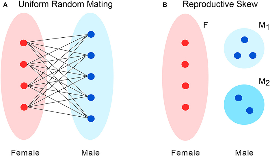
Figure 2. Two models of mating patterns. (A) For uniform random mating, at any given time-step, one male and one female are chosen uniformly to mate to produce an offspring that replaces one individual in the population. However, the sex ratio may be uneven, giving individuals of one sex greater chances for mating. (B) In a model of reproductive skew, males are divided into two subgroups: M₁ and M₂. Each M₁ males is r times as likely to be selected for mating as an M₂ male.

Each time-step, one male and one female are chosen, uniformly at random within each sex, to mate and produce a single offspring. Each offspring replaces a single individual, with each male having probability D_M to be replaced, and each female having probability D_F. Since exactly one individual is replaced, D_M and D_F are constrained by the relationship

$\begin{array}{ll}m{D}_M+f{D}_F=1.& (10)\end{array}$

We treat D_M and D_F as tunable parameters in this model, subject to the above constraint. We observe that D_M and D_F are equal to the marginal probability that an individual (male or female, respectively) is replaced in one time-step, in accordance with the definition of D_I in Section 2.1.

The mating and replacement probabilities $E_{IJ}^K$ are then obtained by multiplying the probability that a specific male-female pair is chosen ($\frac{1}{mf}$) by the probability that the offspring replaces a specific male or female individual (D_M or D_F, respectively). This leads to two distinct values, depending on the sex of the replaced individual:

$\begin{array}{ll}{E}_{MF}^{M^{\prime }}=\frac{1}{mf}{D}_M,E_{MF}^{F^{\prime }}=\frac{1}{mf}{D}_F.& (11)\end{array}$

The primes in M′ and F′ distinguish the replaced individual from the parent of the same sex.

Since a single individual is replaced each time-step, the overall replacement rate is B = 1. For the birth rate of an individual from each sex, we have

$\begin{array}{ll}\begin{array}{c}{B}_M=\frac{1}{2}\left(mf{E}_{MF}^{M^{\prime }}+f^2{E}_{MF}^{F^{\prime }}\right)=\frac{1}{2m}\\ B_F=\frac{1}{2}\left(m^2{E}_{MF}^{M^{\prime }}+mf{E}_{MF}^{F^{\prime }}\right)=\frac{1}{2f},\end{array}& (12)\end{array}$

reflecting the fact that exactly one individual from each sex is chosen to mate.

Since each new offspring replaces a deceased individual, the offspring born in each time-step is male with probability mD_M and female with probability fD_F. The sex ratio at birth is therefore (mD_M)/(fD_F). This may differ from the adult sex ratio of m/f due to differential mortality.

4.1. Deriving fixation probability

Since members of each sex are interchangeable, there are only two cases of the recurrence relation for reproductive values, Eq. (5):

$\begin{array}{ll}{D}_M{\rho }_M=\frac{1}{2}(fm{E}_{MF}^{M^{\prime }}{\rho }_M+f^2{E}_{MF}^{F^{\prime }}{\rho }_F)& (\mathrm{13a})\end{array}$

$\begin{array}{ll}{D}_F{\rho }_F=\frac{1}{2}(m^2{E}_{MF}^{M^{\prime }}{\rho }_M+fm{E}_{MF}^{F^{\prime }}{\rho }_F).& (\mathrm{13b})\end{array}$

Upon substituting from Eq. (11), both equations in Eq. (13) simplify to

$\begin{array}{ll}m{D}_M{\rho }_M=f{D}_F{\rho }_F.& (14)\end{array}$

This means that the reproductive values of the sexes are in inverse ratio to their frequencies at birth: ρ_M/ρ_F = (fD_F)/(mD_M). Meanwhile, Eq. (6) becomes

$\begin{array}{ll}2(m{\rho }_M+f{\rho }_F)=1,& (15)\end{array}$

Solving Eqs. (14) and (15) yields:

$\begin{array}{ll}{\rho }_F=\frac{D_M}{2f(D_M+D_F)},{\rho }_M=\frac{D_F}{2m(D_M+D_F)}.& (16)\end{array}$

Substituting into Eq. (7) gives the overall fixation probability:

$\begin{array}{ll}\rho =m{D}_M{\rho }_M+f{D}_F{\rho }_F=\frac{D_M{D}_F}{D_M+D_F}.& (17)\end{array}$

This solution is illustrated in Figure 3.

FIGURE 3

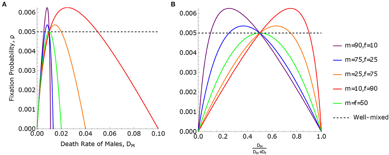
Figure 3. Fixation probabilities in the uneven sex ratio model. Fixation probability, ρ Eq. 7, for the uneven sex ratio model is plotted against (A) the death rate of males, D_M, and (B) the relative death rate of males, $\frac{D_M}{D_M+D_F}$. The total population size is N = m + f = 100. In panel B, the relative death rate, $\frac{D_M}{D_M+D_F}$, is used to highlight the symmetry between males and females, where D_M < D_F when the curves are to the left of x = 0.5 and opposite to the right. The maximum point of each curve is determined by Eq. (22). The curves in (A, B) all pass through the line ρ = ρ_WM twice, with the exception of the case m = f = 50. One intersection point, which is the same for all curves, occurs when $D_M=D_F=\frac{1}{50}$, demonstrating Result 1. The second intersection point occurs when $B_M=D_M=\frac{1}{2m}$. This is a case of Result 2, where ρ = ρ_WM when the birth and death rates are equal, and is different in each curve. Result 3 applies to the case where m = f = 50. In this case, ρ can never be greater than the well-mixed population, ρ_WM, meaning the birth rates of males and females are equal and $B_M=B_F=\frac{1}{100}$.

4.2. Comparing to well-mixed population

Since the fixation probability in a well-mixed population is ${\rho }_{\text{WM}}=\frac{1}{2N}=\frac{1}{2(m+f)}$, we have ρ > ρ_WM if and only if

$\begin{array}{ll}\frac{D_M{D}_F}{D_M+D_F}>\frac{1}{2(m+f)}.& (18)\end{array}$

Applying Eq. (10), this condition simplifies to

$\begin{array}{ll}(D_M-D_F)(m{D}_M-f{D}_F)<0.& (19)\end{array}$

We conclude that the fixation probability is unchanged from the baseline value, ρ = ρ_WM, if either D_M = D_F (equal turnover per sex) or mD_M = fD_F (equal sex ratio at birth). The first case is an instance of Result 1, i.e., ρ = ρ_WM if each individual is replaced at the same rate. In the second case, Eqs. (10) and (12) imply

$\begin{array}{ll}{D}_M=B_M=\frac{1}{2m},D_F=B_F=\frac{1}{2f}.& (20)\end{array}$

This is an instance of Result 2, i.e., ρ = ρ_WM if each individual has birth rate equal to death rate. In this case, since the sex ratio is equal at birth (mD_M = fD_F), any bias in the adult sex ratio is solely due to differential survival. The minority sex gains an advantage in reproduction, but this is exactly canceled by their higher mortality, leading to equal reproductive values, ρ_M = ρ_F.

According to Eq. (19), ρ > ρ_WM (meaning the rate of neutral substitution is accelerated) if and only if D_M − D_F and mD_M − fD_F have opposite signs, meaning that the minority sex at birth has higher mortality. Conversely, if the minority sex at birth has lower mortality, then ρ < ρ_WM and the rate of neutral substitution is slowed. This can be seen in Figure 3. We observe that if m = f, the two solutions to ρ = ρ_WM coincide, and ρ ≤ ρ_WM with equality if and only if D_M = D_F. This is an instance of Result 3, since B_M = B_F when m = f.

4.3. Maximizing fixation probability

To determine the extent to which the fixation probability ρ can deviate from its well-mixed value, we apply Lagrange multipliers to Eq. (16), with D_M and D_F as variables and Eq. (10) as a constraint. This leads to a critical point of

$\begin{array}{ll}{D}_M=\frac{1}{\sqrt{m}(\sqrt{f}+\sqrt{m})},D_F=\frac{1}{\sqrt{f}(\sqrt{f}+\sqrt{m})}.& (21)\end{array}$

Substituting into Eq. (17), we obtain the maximal fixation probability:

$\begin{array}{ll}{\rho }_{\text{MAX}}=\frac{1}{{(\sqrt{f}+\sqrt{m})}^2}.& (22)\end{array}$

This maximal value corresponds to the peaks of the curves in Figure 3.

The ratio of ρ_MAX to ρ_WM can be written in terms of the sex ratio m/f:

$\begin{array}{ll}\frac{{\rho }_{\text{MAX}}}{{\rho }_{\text{WM}}}=\frac{2(f+m)}{{(\sqrt{f}+\sqrt{m})}^2}=\frac{2(1+\frac{m}{f})}{{\left(1+\sqrt{\frac{m}{f}}\right)}^2}.& (23)\end{array}$

As the sex ratio approaches either zero or infinity (the two possible extremes), the ratio ρ_MAX/ρ_WM converges to 2. Thus, under extreme sex ratios, the rate of neutral substitution may be accelerated (relative to the well-mixed population) by a factor of up to two.

5. Scenario 2: Reproductive skew

We next consider a model of reproductive skew (Johnstone, 2000; Nonacs and Hager, 2011), meaning that a subset of one sex dominates reproduction. Reproductive skew arises in many bird species (Petrie et al., 1991; Magrath et al., 2004), as well as in social insects (Adams and Atkinson, 2008; Shimoji and Dobata, 2022), some mammals (Boesch et al., 2006; Raihani and Clutton-Brock, 2010; Sherman et al., 2017; Higham et al., 2021), and snapping shrimp (Synalpheus; Chak et al., 2015).

In presenting the model we will refer to reproductive skew in males, but the labels “male” and “female” are arbitrary, and the results apply equally to skew in either sex.

As in the earlier scenario, we consider a population consisting of a set M of males and a set F of females. In this case, however, the males are partitioned into two subsets, M₁ and M₂, where M₁ males have a greater chance of reproducing. Specifically, the reproductive rate of M₁ males exceeds that of M₂ males by a factor r > 1. The numbers of M₁ males, M₂ males, and females are denoted m₁, m₂, and f respectively. The total population size is N = m₁ + m₂ + f.

Each time-step, a single offspring is produced by a single male-female pair. Each particular M₁ male has probability r/(rm₁ + m₂) to reproduce, while each particular M₂ male has probability 1/(rm₁ + m₂). Each female has probability 1/f to reproduce. This new offspring replaces a deceased adult; each M₁ male, M₂ male, and female has probability D_M1, D_M2, and D_F, respectively, to be replaced in a given time-step. Since exactly one individual is replaced, these death probabilities are constrained by

$\begin{array}{ll}{m}_1{D}_{M_1}+m_2{D}_{M_2}+f{D}_F=1.& (24)\end{array}$

Since the new offspring replaces the deceased adult, the new offspring is a M₁ male, M₂ male, or female with respective probabilities m₁D_M1, m₂D_M2, or fD_F. In particular, the sex ratio at birth is (m₁D_M1 + m₂D_M2)/(fD_F).

From this model description, we derive the following probabilities for a specific male-female pair to replace a specific individual:

$\begin{array}{ll}{E}_{M_{1}F}^{{M_1}^{\prime }}=\left(\frac{r}{r{m}_1+m_2}\right)\left(\frac{1}{f}\right)D_{M_1}& (\mathrm{25a})\end{array}$

$\begin{array}{ll}{E}_{M_{1}F}^{M_2}=\left(\frac{r}{r{m}_1+m_2}\right)\left(\frac{1}{f}\right)D_{M_2}& (\mathrm{25b})\end{array}$

$\begin{array}{ll}{E}_{M_{1}F}^{F^{\prime }}=\left(\frac{r}{r{m}_1+m_2}\right)\left(\frac{1}{f}\right)D_F& (\mathrm{25c})\end{array}$

$\begin{array}{ll}{E}_{M_{2}F}^{M_1}=\left(\frac{1}{r{m}_1+m_2}\right)\left(\frac{1}{f}\right)D_{M_1}& (\mathrm{25d})\end{array}$

$\begin{array}{ll}{E}_{M_{2}F}^{{M_2}^{\prime }}=\left(\frac{1}{r{m}_1+m_2}\right)\left(\frac{1}{f}\right)D_{M_2}& (25e)\end{array}$

$\begin{array}{ll}{E}_{M_{2}F}^{F^{\prime }}=\left(\frac{1}{r{m}_1+m_2}\right)\left(\frac{1}{f}\right)D_F.& (\mathrm{25f})\end{array}$

Each probability $E_{IJ}^K$ is the product of three probabilities: that of choosing a male for reproduction, choosing a female for reproduction, and choosing an individual for replacement.

5.1. Deriving fixation probability

For this model, the recurrence equation for fixation probabilities, Eq. (5), becomes

$\begin{array}{ll}{D}_{M_1}{\rho }_{M_1}=\frac{1}{2}\left(f{m}_1{E}_{M_{1}F}^{{M_1}^{\prime }}{\rho }_{M_1}+f{m}_2{E}_{M_{1}F}^{M_2}{\rho }_{M_2}+f^2{E}_{M_{1}F}^{F^{\prime }}{\rho }_F\right)& (\mathrm{26a})\end{array}$

$\begin{array}{ll}{D}_{M_2}{\rho }_{M_2}=\frac{1}{2}\left(f{m}_2{E}_{M_{2}F}^{{M_2}^{\prime }}{\rho }_{M_1}+f{m}_1{E}_{M_{2}F}^{M_1}{\rho }_{M_2}+f^2{E}_{M_{2}F}^{F^{\prime }}{\rho }_F\right)& (\mathrm{26b})\end{array}$

$\begin{array}{l}{D}_F{\rho }_F=\frac{1}{2}(m_1^2{E}_{M_{1}F}^{M_1\prime }{\rho }_{M_1}+m_1{m}_2{E}_{M_{1}F}^{M_2}{\rho }_{M_1}+m_{1}f{E}_{M_{1}F}^{F^{\prime }}{\rho }_{M_1}+\hfill \\ m_2^2{E}_{M_{2}F}^{M_2\prime }{\rho }_{M_2}+m_2{m}_1{E}_{M_{2}F}^{M_1}{\rho }_{M_2}+m_{2}f{E}_{M_{2}F}^{F^{\prime }}{\rho }_{M_2}).\hfill & (\mathrm{26c})\end{array}$

Substituting the marginal probabilities from Eq. (25), Eqs. (26a) and (26b) simplify to

$\begin{array}{ll}2(r{m}_1+m_2)D_{M_1}{\rho }_{M_1}=r{m}_1{D}_{M_1}{\rho }_{M_1}+r{m}_2{D}_{M_2}{\rho }_{M_2}+rf{D}_F{\rho }_F& (\mathrm{27a})\end{array}$

$\begin{array}{ll}2(r{m}_1+m_2)D_{M_2}{\rho }_{M_2}=m_1{D}_{M_1}{\rho }_{M_1}+m_2{D}_{M_2}{\rho }_{M_2}+f{D}_F{\rho }_F.& (\mathrm{27b})\end{array}$

Observing that Eqs. (27a) and (27b) differ only in a factor of r on the right hand side, we conclude that

$\begin{array}{ll}{D}_{M_1}{\rho }_{M_1}=r{D}_{M_2}{\rho }_{M_2}.& (28)\end{array}$

This reduces Eq. (27a) to

$\begin{array}{ll}(r{m}_1+m_2)D_{M_1}{\rho }_{M_1}=rf{D}_F{\rho }_F.& (29)\end{array}$

Meanwhile, Eq. (6) gives

$\begin{array}{ll}2(m_1{\rho }_{M_1}+m_2{\rho }_{M_2}+f{\rho }_F)=1.& (30)\end{array}$

Solving the system of equations formed by Eqs. (28)–(30), we obtain the solution

$\begin{array}{ll}{\rho }_{M_1}=\frac{r{D}_{M_1}{D}_F}{2(m_{1}r{D}_{M_2}{D}_F+m_2{D}_{M_1}{D}_F+(r{m}_1+m_2)D_{M_1}{D}_{M_2})}& (\mathrm{31a})\end{array}$

$\begin{array}{ll}\begin{array}{c}{\rho }_{M_2}=\frac{D_{M_1}{D}_F}{2(m_{1}r{D}_{M_2}{D}_F+m_2{D}_{M_1}{D}_F+(r{m}_1+m_2)D_{M_1}{D}_{M_2})}\end{array}& (\mathrm{31b})\end{array}$

$\begin{array}{ll}\begin{array}{c}{\rho }_F=\frac{(r{m}_1+m_2)D_{M_1}{D}_{M_2}}{2f(m_{1}r{D}_{M_2}{D}_F+m_2{D}_{M_1}{D}_F+(r{m}_1+m_2)D_{M_1}{D}_{M_2})}.\end{array}& (\mathrm{31c})\end{array}$

The overall fixation probability is therefore

$\begin{array}{l}\rho =m_1{D}_{M_1}{\rho }_{M_1}+m_2{D}_{M_2}{\rho }_{M_2}+f{D}_F{\rho }_F\\ =\frac{(r{m}_1+m_2)D_{M_1}{D}_{M_2}{D}_F}{m_{1}r{D}_{M_2}{D}_F+m_2{D}_{M_1}{D}_F+(r{m}_1+m_2)D_{M_1}{D}_{M_2}}.& (32)\end{array}$

For r = 1 and D_M1 = D_M2, Eq. (32) reduces to Eq. (17) for the uneven sex ratio model, with D_M = D_M1 = D_M2 and m = m₁ + m₂. This reflects the fact that when M₁ and M₂ males are interchangeable, the two models become equivalent.

5.2. Comparing to well-mixed population

Comparing our solution for ρ in Eq. (32) to the fixation probability in a well-mixed population of the same size, ρ_WM = 1/(2N) = 1/(2m₁ + 2m₂ + 2f), we find that ρ > ρ_WM is equivalent to

$\begin{array}{ll}2(r{m}_1+m_2)(m_1+m_2+f)>\frac{r{m}_1+m_2}{D_F}+\frac{r{m}_1}{D_{M_1}}+\frac{m_2}{D_{M_2}}.& (33)\end{array}$

To simplify, let us suppose that the sex ratio is even both for adults, f = m₁ + m₂, and at birth, $m_1{D}_{M_1}+m_2{D}_{M_2}=f{D}_F=\frac{1}{2}$. Then Condition (33) reduces to

$\begin{array}{ll}2(r{m}_1+m_2)(m_1+m_2)>\frac{r{m}_1}{D_{M_1}}+\frac{m_2}{D_{M_2}}.& (34)\end{array}$

Simplifying using the relation $m_1{D}_{M_1}+m_2{D}_{M_2}=\frac{1}{2}$, we obtain that ρ > ρ_WM if and only if

$\begin{array}{ll}(D_{M_1}-D_{M_2})(D_{M_1}-r{D}_{M_2})<0.& (35)\end{array}$

There are two cases where ρ = ρ_WM, corresponding to the two factors of the left-hand side of Condition (35). Setting the first factor equal to zero leads to

$\begin{array}{ll}{D}_{M_1}=D_{M_2}=D_F=\frac{1}{2(m_1+m_2)}=\frac{1}{2f}.& (36)\end{array}$

This is an example of Result 1 from Section 3.2.

Setting the second factor of the left-hand side of Condition (35) equal to zero leads to

$\begin{array}{ll}{D}_{M_1}=B_{M_1}=\frac{r}{2(r{m}_1+m_2)}& (\mathrm{37a})\end{array}$

$\begin{array}{ll}{D}_{M_2}=B_{M_2}=\frac{1}{2(r{m}_1+m_2)}& (\mathrm{37b})\end{array}$

$\begin{array}{ll}{D}_F=B_F=\frac{1}{2(m_1+m_2)}.& (\mathrm{37c})\end{array}$

This is an example of Result 2, in that each individual has birth rate equal to its replacement rate.

According to Condition (35), ρ > ρ_WM (meaning the neutral substitution rate is accelerated) when D_M1 lies between D_M2 and rD_M2. This arises when M₁ males have higher mortality than M₂ males, but not so high as to negate their reproductive advantage. If D_M1 is smaller than D_M2 or larger than rD_M2, then ρ < ρ_WM and the neutral substitution rate is slowed. This can be seen in Figure 4, where the solution in Eq. (36) is the common intersection point for all curves, while the solution in Eq. (37) varies depending on the parameters.

FIGURE 4

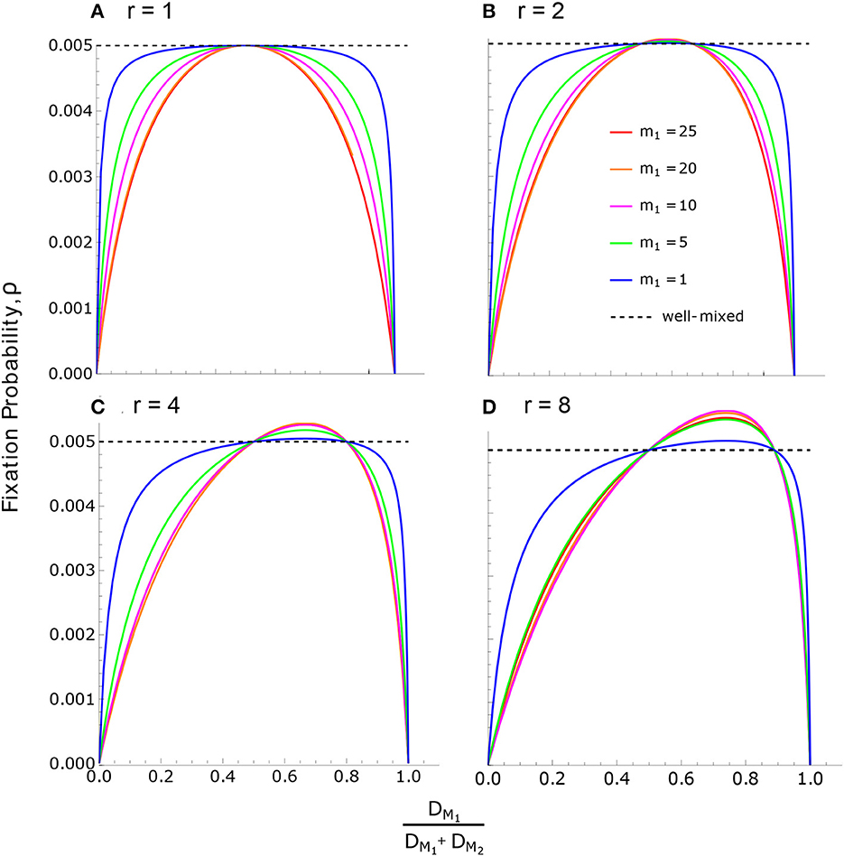
Figure 4. Neutral fixation probability in the reproductive skew model. Fixation probability, according to Eq. (32), is plotted against $\frac{D_{M_1}}{D_{M_1}+D_{M_2}}$ for various values of m₁ and r. In all cases, there are 50 individuals of each sex, m₁ + m₂ = f = 50, and the sex ratio is even at birth, $m_1{D}_{M_1}+m_2{D}_{M_2}=f{D}_F=\frac{1}{2}$. (A) For r = 1, all birth rates are equal (B_M1 = B_M2 = B_F), and therefore ρ ≤ ρ_WM as a consequence of Result 3. Note that equality, ρ = ρ_WM, occurs only when death rates are also equal across individuals. (B–D) The effects of increasing r. The maximum value of ρ for each curve is given by Eq. (49).

5.3. Maximizing fixation probability

To determine how widely the fixation probability can vary for fixed m₁, m₂, f, and r, we seek a maximum of the function

$\begin{array}{l}\rho (D_{M_1},D_{M_2},D_F)\\ =\frac{(r{m}_1+m_2)D_{M_1}{D}_{M_2}{D}_F}{m_{1}r{D}_{M_2}{D}_F+m_2{D}_{M_1}{D}_F+(r{m}_1+m_2)D_{M_1}{D}_{M_2}}.& (38)\end{array}$

subject to the constraint of Eq. (24). Applying Lagrange multipliers gives the equations

$\begin{array}{l}\frac{\partial \rho }{\partial D_{M_1}}=\frac{(r{m}_1+m_2)r{m}_1{D}_{M_2}^2{D}_F^2}{{((r{m}_1+m_2)D_{M_1}{D}_{M_2}+r{m}_1{D}_{M_2}{D}_F+m_2{D}_{M_1}{D}_F)}^2}\\ =\lambda m_1& (\mathrm{39a})\end{array}$

$\begin{array}{l}\frac{\partial \rho }{\partial D_{M_2}}=\frac{(r{m}_1+m_2)m_2{D}_{M_1}^2{D}_F^2}{{((r{m}_1+m_2)D_{M_1}{D}_{M_2}+r{m}_1{D}_{M_2}{D}_F+m_2{D}_{M_1}{D}_F)}^2}\\ =\lambda m_2& (\mathrm{39b})\end{array}$

$\begin{array}{l}\frac{\partial \rho }{\partial D_F}=\frac{{(r{m}_1+m_2)}^2{D}_{M_1}^2{D}_{M_2}^2}{{((r{m}_1+m_2)D_{M_1}{D}_{M_2}+r{m}_1{D}_{M_2}{D}_F+m_2{D}_{M_1}{D}_F)}^2}\\ =\lambda f.& (\mathrm{39c})\end{array}$

Dividing (39a) by (39b) and simplifying gives

$\begin{array}{ll}{D}_{M_1}=\sqrt{r}{D}_{M_2},& (40)\end{array}$

while dividing (39a) by (39c) yields

$\begin{array}{ll}\sqrt{rf}{D}_F=\sqrt{r{m}_1+m_2}{D}_{M_1}.& (41)\end{array}$

Invoking (24) and solving, we obtain the maximizing values

$\begin{array}{ll}{D}_{M_1}=\frac{\sqrt{r}}{m_1\sqrt{r}+m_2+\sqrt{f(r{m}_1+m_2)}}& (\mathrm{42a})\end{array}$

$\begin{array}{ll}{D}_{M_2}=\frac{1}{m_1\sqrt{r}+m_2+\sqrt{f(r{m}_1+m_2)}}& (\mathrm{42b})\end{array}$

$\begin{array}{ll}{D}_F=\frac{\sqrt{(r{m}_1+m_2)}}{\sqrt{f}\left(m_1\sqrt{r}+m_2+\sqrt{f(r{m}_1+m_2)}\right)}.& (\mathrm{42c})\end{array}$

Substituting these expressions into (38) gives the maximal fixation probability of

$\begin{array}{ll}{\rho }_{\text{MAX}}=\frac{r{m}_1+m_2}{{(m_1\sqrt{r}+m_2+\sqrt{f(r{m}_1+m_2})}^2}.& (43)\end{array}$

Comparing to the well-mixed population, we find the ratio of fixation probabilities is given by

$\begin{array}{ll}\frac{{\rho }_{\text{MAX}}}{{\rho }_{\text{WM}}}=\frac{2(m_1+m_2+f)(r{m}_1+m_2)}{{\left(\sqrt{f(r{m}_1+m_2)}+m_1\sqrt{r}+m_2\right)}^2}.& (44)\end{array}$

To determine the most extreme values of fixation probability, we take r → ∞ in Eq. (43), yielding

$\begin{array}{ll}{\displaystyle \underset{r\to \infty }{lim}}{\rho }_{\text{MAX}}=\frac{1}{{(\sqrt{m_1}+\sqrt{f})}^2}.& (45)\end{array}$

This is equivalent to Eq. (22) with m replaced by m₁, since for r → ∞ only M₁ males have the opportunity to reproduce. In this case, an arbitrarily large ratio ρ_MAX/ρ_WM can be achieved by considering a large number of M₂ males:

$\begin{array}{ll}{\displaystyle \underset{m_2\to \infty }{lim}}{\displaystyle \underset{r\to \infty }{lim}}\frac{{\rho }_{\text{MAX}}}{{\rho }_{\text{WM}}}={\displaystyle \underset{m_2\to \infty }{lim}}\frac{2(m_1+m_2+f)}{{(\sqrt{m_1}+\sqrt{f})}^2}=\infty .& (46)\end{array}$

5.4. Maximization under even sex ratio

The preceding section shows that, in our reproductive skew model, the neutral substitution rate may be scaled by any positive factor relative to the well-mixed rate. However, this is achieved only with an extreme male-biased sex ratio, in that m₂ is taken to infinity with m₁ and f held constant. It is also of interest to determine how widely the neutral substitution rate can vary when the overall sex ratio is held even, both at birth and among adults. This is the case depicted in Figure 4.

To this end, we seek to maximize ρ under the constraints that the sex ratio is even among adults, m₁ + m₂ = f, and at birth, $m_1{D}_{M_1}+m_2{D}_{M_2}=f{D}_F=\frac{1}{2}$. Together, these constraints imply D_F = 1/(2(m₁ + m₂)). Substituting this into Eq. (32) and simplifying, we obtain

$\begin{array}{ll}\rho =\frac{r{m}_1+m_2}{r{m}_1{D}_{M_1}^{-1}+m_2{D}_{M_2}^{-1}+2(m_1+m_2)(r{m}_1+m_2)}.& (47)\end{array}$

To maximize ρ, we apply Lagrange multipliers in the variables D_M1 and D_M2 with the constraint m₁D_M1 + m₂D_M2 = 1/2. We obtain that ρ is maximized when $D_{M_1}=\sqrt{r}{D}_{M_2}$; specifically,

$\begin{array}{ll}{D}_{M_1}=\frac{\sqrt{r}}{2\left(m_1\sqrt{r}+m_2\right)}& (\mathrm{48a})\end{array}$

$\begin{array}{ll}{D}_{M_2}=\frac{1}{2\left(m_1\sqrt{r}+m_2\right)}.& (\mathrm{48b})\end{array}$

Substituting in Eq. (47) gives the maximal fixation probability under these constraints:

$\begin{array}{ll}{\rho }_{\text{MAX}}=\frac{r{m}_1+m_2}{2{\left(m_1\sqrt{r}+m_2\right)}^2+2(m_1+m_2)(r{m}_1+m_2)}.& (49)\end{array}$

Eqs. (48)–(49) correspond to the maxima of the curves depicted in Figure 4. Comparing to well-mixed value of ρ_WM = 1/(4(m₁ + m₂)), we have

$\begin{array}{ll}\frac{{\rho }_{\text{MAX}}}{{\rho }_{\text{WM}}}=\frac{2\left(m_1+m_2\right)(r{m}_1+m_2)}{{(m_1\sqrt{r}+m_2)}^2+(m_1+m_2)(r{m}_1+m_2)}.& (50)\end{array}$

In the extreme scenario r → ∞, in which M₁ males completely dominate reproduction, we obtain

$\begin{array}{ll}{\displaystyle \underset{r\to \infty }{lim}}\frac{{\rho }_{\text{MAX}}}{{\rho }_{\text{WM}}}=\frac{2(m_1+m_2)}{2m_1+m_2}.& (51)\end{array}$

If, in addition, we take the ratio m₁/m₂ to zero (meaning M₁ males are a very small minority), then ρ_MAX/ρ_WM converges to 2, which is an upper bound for ρ_MAX/ρ_WM in the case of even sex ratios at birth and in adults.

6. Discussion

For the fixation probability of a neutral mutation to differ from the well-mixed of ${\rho }_{\text{WM}}=\frac{1}{2N}$, three conditions must be met. First, the rates of replacement D_I must vary across individuals (or classes of individuals), or else ρ = ρ_WM by Result 1. Second, the reproductive values ρ_I must vary across individuals; by Result 2 this occurs if and only if at least one individual (or class) has birth rate not equal to its death rate. Third, the variation in D_I and ρ_I must be correlated, so that $\frac{1}{N}\sum _I{D}_I{\rho }_I$ differs from $(\frac{1}{N}\sum _I{D}_I)(\frac{1}{N}\sum _I{\rho }_I)$. If these three conditions are met, Kimura's (1968) result K = u—which underlies the molecular clock hypothesis (Kimura, 1983; Ayala, 1997; Bromham and Penny, 2003; Kumar, 2005)—requires a correction factor of ρ/ρ_WM. For a diploid population of size N, the corrected rate of neutral substitution is K = 2Nρu.

A key assumption underlying our results is that mutation occurs with constant probability per birth. This fact, combined with unequal replacement rates, means that mutations are more likely to arise in certain subgroups rather than others; if these subgroups also have larger-than-average reproductive value, then the rate of neutral substitution will be accelerated.

It has previously been shown that the rate of genetic substitution can be affected by selection, varying population size (Balloux and Lehmann, 2012), mutation rates that vary by age or sex (Pollak, 1982; Charlesworth, 1994; Lehmann, 2014), or asymmetric spatial structure (Allen et al., 2015). To this list we now add uneven sex ratio, reproductive skew, and other asymmetric mating patterns, in combination with unequal replacement rates.

For uneven sex ratio, the correction factor ρ/ρ_WM can take any value strictly between 0 to 2 (Figure 3). Deviations from the well-mixed rate occur when there is both differential survival, D_M ≠ D_F, and unequal sex ratio at birth, mD_M ≠ fD_F. If the minority sex at birth has higher (resp., lower) mortality, the neutral substitution rate is accelerated (resp., slowed). According to Eq. (21), the maximal substitution rate occurs when the ratio of replacement rates is inversely proportional to the square root of the sex ratio, $D_M/D_F=\sqrt{f/m}$—or equivalently, when the adult sex ratio is the square of the sex ratio at birth, $m/f={(m{D}_M)}^2/{(f{D}_F)}^2$.

In order to affect the neutral substitution rate in our model, the uneven sex ratio must arise at birth. If, instead, the uneven sex ratio is solely due to differential survival, then the reproductive advantage of the minority sex is canceled by their higher mortality. This limits the range of taxa for which such effects may arise, since unequal sex ratios at birth violate random Mendelian segregation as well as Fisher's (Fisher, 1930) principle that sex ratios should evolve toward unity. Although most bird species have even sex ratio at birth (Donald, 2007), exceptions have been observed, for example, in some tit species (Cichoń et al., 2005) and in collared flycatchers (Ficedula albicollis; Rosivall et al., 2004; Cichoń et al., 2005). A richer source of possible examples are reptiles with temperature-dependent sex determination (Ferguson and Joanen, 1982; Ewert and Nelson, 1991; Lang and Andrews, 1994; Mrosovsky, 1994; González et al., 2019), which often have uneven sex ratio under baseline environmental conditions (Ferguson and Joanen, 1982; Ewert and Nelson, 1991).

For reproductive skew, the correction factor ρ/ρ_WM can take any positive value. If we additionally specify that the sex ratio is even at birth and among adults, then ρ/ρ_WM varies strictly between 0 and 2. Acceleration of the neutral substitution rate occurs when D_M1 lies between D_M2 and rD_M2, meaning that the dominant reproducers have higher mortality than others of their sex, but not so high as to negate their reproductive advantage.

Reproductive skew arises in many taxa (Raihani and Clutton-Brock, 2010), including numerous bird species (Wiley, 1973; Petrie et al., 1991; Höglund and Alatalo, 1995; Magrath et al., 2004), social insects (Adams and Atkinson, 2008; Shimoji and Dobata, 2022), non-human primates (Boesch et al., 2006; Higham et al., 2021), meerkats (Suricata suricatta; Clutton-Brock et al., 2001), naked mole rats (Heterocephalus glaber; Sherman et al., 2017), and snapping shrimp (Synalpheus; Chak et al., 2015). For the rate of neutral substitution to be altered, reproductive success must correlate (positively or negatively) with mortality. There are many ways such a correlation may arise. Dominant reproducers may be more physically robust (Hodge et al., 2008) and so may survive longer; on the other hand, they may experience greater mortality due to competition (Leimar and Bshary, 2022). For the northern mole-vole Ellobius talpinus Pall., Novikov et al. (2015) found that mortality is negatively correlated with reproduction; in this case, our model predicts a slower-than-baseline neutral substitution rate.

Here we have considered effects due to sex and space, but not age. The age structure of a population has clear implications for its neutral substitution rate (Pollak, 1982; Charlesworth, 1994; Lehmann, 2014). Investigating the combined effects of age, sex, and spatial structure is a promising avenue for future work. Incorporating age structure would also allow for greater realism in applying this framework to real-world populations (Charlesworth, 1994; Sample et al., 2018). Age structure could be incorporated into the framework described in the Supplementary material by designating a fixed subset of individuals to be juveniles. The mating and replacement probabilities $E_{IJ}^K$ would then be nonzero only if I and J are adults and K is a juvenile. It would also be necessary to specify the probability for each juvenile to survive to adulthood. This would represent a significant—and important—expansion of the mathematical modeling framework developed by Allen and McAvoy (2019).

Our analysis has focused on the rate of neutral substitution at a single genetic locus. It would also be of interest to extend to multiple loci. This would require amending the framework presented in the Supplementary material to keep account of the two alleles at each locus in each (diploid) individual. The probability of recombination in each new offspring would then be a key parameter. Such an expanded framework could bring new methods to bear on the well-studied question of how mating patterns affect linkage disequilibrium (Weir and Cockerham, 1969; Golding and Strobeck, 1980; Nordborg, 2000).

We have also implicitly assumed that the rate of neutral substitution is primarily limited by the appearance rate and fixation probability of neutral mutations. This assumption is reasonable so long as the expected fixation time, T, is significantly less than the waiting time, 1/(2Nuρ), for successful mutations to arise. Outside of this regime, fixation time becomes relevant for the neutral substitution rate (Frean et al., 2013). Fixation times have been studied extensively for spatially structured populations (Frean et al., 2013; Hathcock and Strogatz, 2019; Möller et al., 2019; Tkadlec et al., 2019), and to a lesser extent for populations with asymmetric mating pattern (Paley et al., 2010). Examining the combined effect of fixation probability and time on the rate of neutral substitution, in populations with asymmetric mating pattern, is an interesting avenue for further study.

Data availability statement

The original contributions presented in the study are included in the article/Supplementary material, further inquiries can be directed to the corresponding author.

Author contributions

BA conceived the project. EB, BA, AS, AH, AT, LA, YD, and CS analyzed the model. EB, BA, and CS wrote the manuscript. All authors contributed to the article and approved the submitted version.

Funding

This project was supported by Grant #62220 from the John Templeton Foundation and Award DMS-1715315 from the National Science Foundation.

Conflict of interest

The authors declare that the research was conducted in the absence of any commercial or financial relationships that could be construed as a potential conflict of interest.

Publisher's note

All claims expressed in this article are solely those of the authors and do not necessarily represent those of their affiliated organizations, or those of the publisher, the editors and the reviewers. Any product that may be evaluated in this article, or claim that may be made by its manufacturer, is not guaranteed or endorsed by the publisher.

Author disclaimer

Opinions expressed by the authors do not necessarily reflect the views of the funding agencies.

Supplementary material

The Supplementary Material for this article can be found online at: https://www.frontiersin.org/articles/10.3389/fevo.2023.1017369/full#supplementary-material

References

Adams, E. S., and Atkinson, L. (2008). Queen fecundity and reproductive skew in the termite nasutitermes corniger. Insectes Sociaux 55, 28–36. doi: 10.1007/s00040-007-0970-5

CrossRef Full Text | Google Scholar

Allen, B., and McAvoy, A. (2019). A mathematical formalism for natural selection with arbitrary spatial and genetic structure. J. Math. Biol. 78, 1147–210. doi: 10.1007/s00285-018-1305-z

PubMed Abstract | CrossRef Full Text | Google Scholar

Allen, B., Sample, C., Dementieva, Y., Medeiros, R. C., Paoletti, C., and Nowak, M. A. (2015). The molecular clock of neutral evolution can be accelerated or slowed by asymmetric spatial structure. PLoS Comput. Biol. 11, e1004108. doi: 10.1371/journal.pcbi.1004108

PubMed Abstract | CrossRef Full Text | Google Scholar

Allen, B., and Tarnita, C. E. (2014). Measures of success in a class of evolutionary models with fixed population size and structure. J. Math. Biol. 68, 109–143. doi: 10.1007/s00285-012-0622-x

PubMed Abstract | CrossRef Full Text | Google Scholar

Ayala, F. J. (1997). Vagaries of the molecular clock. Proc. Natl. Acad. Sci. USA. 94, 7776–7783. doi: 10.1073/pnas.94.15.7776

PubMed Abstract | CrossRef Full Text | Google Scholar

Balloux, F., and Lehmann, L. (2012). Substitution rates at neutral genes depend on population size under fluctuating demography and overlapping generations. Evolution 66, 605–611. doi: 10.1111/j.1558-5646.2011.01458.x

PubMed Abstract | CrossRef Full Text | Google Scholar

Benito, M., and González-Solís, J. (2007). Sex ratio, sex-specific chick mortality and sexual size dimorphism in birds. J. Evol. Biol. 20, 1522–1530. doi: 10.1111/j.1420-9101.2007.01327.x

PubMed Abstract | CrossRef Full Text | Google Scholar

Boesch, C., Kohou, G., Néné, H., and Vigilant, L. (2006). Male competition and paternity in wild chimpanzees of the taï forest. Am. J. Phys. Anthropol. 130, 103–115. doi: 10.1002/ajpa.20341

PubMed Abstract | CrossRef Full Text | Google Scholar

Bromham, L., and Penny, D. (2003). The modern molecular clock. Nat. Rev. Genet. 4, 216–224. doi: 10.1038/nrg1020

PubMed Abstract | CrossRef Full Text | Google Scholar

Chak, S. T. C., Duffy, J. E., and Rubenstein, D. R. (2015). Reproductive skew drives patterns of sexual dimorphism in sponge-dwelling snapping shrimps. Proc. R. Soc. B Biol. Sci. 282, 20150342. doi: 10.1098/rspb.2015.0342

PubMed Abstract | CrossRef Full Text | Google Scholar

Charlesworth, B. (1994). Evolution in Age-Structured Populations, Volume 2. Cambridge: Cambridge University Press. doi: 10.1017/CBO9780511525711

CrossRef Full Text | Google Scholar

Cichoń, M., Sendecka, J., and Gustafsson, L. (2005). Male-biased sex ratio among unhatched eggs in great tit parus major, blue tit P. caeruleus and collared flycatcher Ficedula albicollis. J. Avian Biol. 36, 386–390. doi: 10.1111/j.0908-8857.2005.03589.x

CrossRef Full Text | Google Scholar

Clutton-Brock, T. H., Brotherton, P. N., Russell, A., O'riain, M., Gaynor, D., Kansky, R., et al. (2001). Cooperation, control, and concession in meerkat groups. Science 291, 478–481. doi: 10.1126/science.291.5503.478

PubMed Abstract | CrossRef Full Text | Google Scholar

Donald, P. F. (2007). Adult sex ratios in wild bird populations. Ibis 149, 671–692. doi: 10.1111/j.1474-919X.2007.00724.x

CrossRef Full Text | Google Scholar

Ewert, M. A., and Nelson, C. E. (1991). Sex determination in turtles: diverse patterns and some possible adaptive values. Copeia 1991, 50–69. doi: 10.2307/1446248

CrossRef Full Text | Google Scholar

Ferguson, M. W., and Joanen, T. (1982). Temperature of egg incubation determines sex in alligator mississippiensis. Nature 296, 850–853. doi: 10.1038/296850a0

PubMed Abstract | CrossRef Full Text | Google Scholar

Fisher, R. (1930). The Genetical Theory of Natural Selection. Oxford: Clarendon Press. doi: 10.5962/bhl.title.27468

CrossRef Full Text | Google Scholar

Frean, M., Rainey, P. B., and Traulsen, A. (2013). The effect of population structure on the rate of evolution. Proc. R. Soc. B Biol. Sci. USA. 280, 1762. doi: 10.1098/rspb.2013.0211

PubMed Abstract | CrossRef Full Text | Google Scholar

Golding, G., and Strobeck, C. (1980). Linkage disequilibrium in a finite population that is partially selfing. Genetics 94, 777–789. doi: 10.1093/genetics/94.3.777

PubMed Abstract | CrossRef Full Text | Google Scholar

González, E. J., Martínez-López, M., Morales-Garduza, M. A., García-Morales, R., Charruau, P., and Gallardo-Cruz, J. A. (2019). The sex-determination pattern in crocodilians: a systematic review of three decades of research. J. Anim. Ecol. 88, 1417–1427. doi: 10.1111/1365-2656.13037

PubMed Abstract | CrossRef Full Text | Google Scholar

Hathcock, D., and Strogatz, S. H. (2019). Fitness dependence of the fixation-time distribution for evolutionary dynamics on graphs. Phys. Rev. E 100, 012408. doi: 10.1103/PhysRevE.100.012408

PubMed Abstract | CrossRef Full Text | Google Scholar

Higham, J. P., Heistermann, M., Agil, M., Perwitasari-Farajallah, D., Widdig, A., and Engelhardt, A. (2021). Female fertile phase synchrony, and male mating and reproductive skew, in the crested macaque. Sci. Rep. 11, 4251. doi: 10.1038/s41598-021-81163-1

PubMed Abstract | CrossRef Full Text | Google Scholar

Hodge, S. J., Manica, A., Flower, T. P., and Clutton-Brock, T. H. (2008). Determinants of reproductive success in dominant female meerkats. J. Anim. Ecol. 2008, 92–102. doi: 10.1111/j.1365-2656.2007.01318.x

PubMed Abstract | CrossRef Full Text | Google Scholar

Höglund, J., and Alatalo, R. V. (1995). Leks. Princeton, NJ: Princeton University Press.

Google Scholar

Johnstone, R. A. (2000). Models of reproductive skew: a review and synthesis (invited article). Ethology 106, 5–26. doi: 10.1046/j.1439-0310.2000.00529.x

CrossRef Full Text | Google Scholar

Kimura, M. (1968). Evolutionary rate at the molecular level. Nature 217, 624–626. doi: 10.1038/217624a0

PubMed Abstract | CrossRef Full Text | Google Scholar

Kimura, M. (1983). The Neutral Theory of Molecular Evolution. Cambridge: Cambridge University Press. doi: 10.1017/CBO9780511623486

CrossRef Full Text | Google Scholar

Kumar, S. (2005). Molecular clocks: four decades of evolution. Nat. Rev. Genet. 6, 654–662. doi: 10.1038/nrg1659

PubMed Abstract | CrossRef Full Text | Google Scholar

Lang, J. W., and Andrews, H. V. (1994). Temperature-dependent sex determination in crocodilians. J. Exp. Zool. 270, 28–44. doi: 10.1002/jez.1402700105

CrossRef Full Text | Google Scholar

Lehmann, L. (2014). Stochastic demography and the neutral substitution rate in class-structured populations. Genetics 197, 351–360. doi: 10.1534/genetics.114.163345

PubMed Abstract | CrossRef Full Text | Google Scholar

Leimar, O., and Bshary, R. (2022). Reproductive skew, fighting costs and winner-loser effects in social dominance evolution. J. Anim. Ecol. 91, 1036–1046. doi: 10.1111/1365-2656.13691

PubMed Abstract | CrossRef Full Text | Google Scholar

Maciejewski, W. (2014). Reproductive value in graph-structured populations. J. Theor. Biol. 340, 285–293. doi: 10.1016/j.jtbi.2013.09.032

PubMed Abstract | CrossRef Full Text | Google Scholar

Magrath, R. D., Johnstone, R. A., and Heinsohn, R. (2004). “Reproductive skew,” in Ecology and Evolution of Cooperative Breeding in Birds, eds W. D. Koenig and J. Dickinson (Cambridge: Cambridge University Press). doi: 10.1017/CBO9780511606816.011

CrossRef Full Text | Google Scholar

Maruyama, T. (1970). On the fixation probability of mutant genes in a subdivided population. Genet. Res. 15, 221–225. doi: 10.1017/S0016672300001543

PubMed Abstract | CrossRef Full Text | Google Scholar

Möller, M., Hindersin, L., and Traulsen, A. (2019). Exploring and mapping the universe of evolutionary graphs identifies structural properties affecting fixation probability and time. Commun. Biol. 2, 1–9. doi: 10.1038/s42003-019-0374-x

PubMed Abstract | CrossRef Full Text

Mrosovsky, N. (1994). Sex ratios of sea turtles. J. Exp. Zool. 270, 16–27. doi: 10.1002/jez.1402700104

CrossRef Full Text | Google Scholar

Nagylaki, T. (1982). Geographical invariance in population genetics. J. Theor. Biol. 99, 159–172. doi: 10.1016/0022-5193(82)90396-4

PubMed Abstract | CrossRef Full Text | Google Scholar

Nonacs, P., and Hager, R. (2011). The past, present and future of reproductive skew theory and experiments. Biol. Rev. 86, 271–298. doi: 10.1111/j.1469-185X.2010.00144.x

PubMed Abstract | CrossRef Full Text | Google Scholar

Nordborg, M. (2000). Linkage disequilibrium, gene trees and selfing: an ancestral recombination graph with partial self-fertilization. Genetics 154, 923–929. doi: 10.1093/genetics/154.2.923

PubMed Abstract | CrossRef Full Text | Google Scholar

Novikov, E., Kondratyuk, E., Petrovski, D., Titova, T., Zadubrovskaya, I., Zadubrovskiy, P., et al. (2015). Reproduction, aging and mortality rate in social subterranean mole voles (Ellobius talpinus pall). Biogerontology 16, 723–732. doi: 10.1007/s10522-015-9592-x

PubMed Abstract | CrossRef Full Text | Google Scholar

Paley, C., Taraskin, S., and Elliott, S. (2010). Assortative mating and mutation diffusion in spatial evolutionary systems. Phys. Rev. E 81, e041912. doi: 10.1103/PhysRevE.81.041912

PubMed Abstract | CrossRef Full Text | Google Scholar

Petrie, M., Tim, H., and Carolyn, S. (1991). Peahens prefer peacocks with elaborate trains. Anim. Behav. 41, 323–331. doi: 10.1016/S0003-3472(05)80484-1

CrossRef Full Text | Google Scholar

Pollak, E. (1982). The rate of mutant substitution in populations with overlapping generations. Genet. Res. 40, 89–94. doi: 10.1017/S0016672300018930

PubMed Abstract | CrossRef Full Text | Google Scholar

Raihani, N. J., and Clutton-Brock, T. H. (2010). Higher reproductive skew among birds than mammals in cooperatively breeding species. Biol. Lett. 6, 630–632. doi: 10.1098/rsbl.2010.0159

PubMed Abstract | CrossRef Full Text | Google Scholar

Rosivall, B., Török, J., Hasselquist, D., and Bensch, S. (2004). Brood sex ratio adjustment in collared flycatchers (Ficedula albicollis): results differ between populations. Behav. Ecol. Sociobiol. 56, 346–351. doi: 10.1007/s00265-004-0796-3

PubMed Abstract | CrossRef Full Text | Google Scholar

Sample, C., Fryxell, J. M., Bieri, J. A., Federico, P., Earl, J. E., Wiederholt, R., et al. (2018). A general modeling framework for describing spatially structured population dynamics. Ecol. Evol. 8, 493–508. doi: 10.1002/ece3.3685

PubMed Abstract | CrossRef Full Text | Google Scholar

Sherman, P. W., Jarvis, J. U., and Alexander, R. D. (2017). The Biology of the Naked Mole-Rat. Princeton, NJ: Princeton University Press. doi: 10.1515/9781400887132

CrossRef Full Text | Google Scholar

Shimoji, H., and Dobata, S. (2022). The build-up of dominance hierarchies in eusocial insects. Philos. Trans. R. Soc. B 377, 20200437. doi: 10.1098/rstb.2020.0437

PubMed Abstract | CrossRef Full Text | Google Scholar

Taylor, P. D. (1990). Allele-frequency change in a class-structured population. Am. Nat. 135, 95–106. doi: 10.1086/285034

CrossRef Full Text | Google Scholar

Tkadlec, J., Pavlogiannis, A., Chatterjee, K., and Nowak, M. A. (2019). Population structure determines the tradeoff between fixation probability and fixation time. Commun. Biol. 2, 1–8. doi: 10.1038/s42003-019-0373-y

PubMed Abstract | CrossRef Full Text | Google Scholar

Weir, B., and Cockerham, C. C. (1969). Pedigree mating with two linked loci. Genetics 61, 923. doi: 10.1093/genetics/61.4.923

PubMed Abstract | CrossRef Full Text | Google Scholar

Wiley, R. H. (1973). Territoriality and non-random mating in sage grouse, centrocercus urophasianus. Anim. Behav. Monogr. 6, 85–169. doi: 10.1016/0003-3472(73)90004-3

CrossRef Full Text | Google Scholar