An objective approach to select surrogate species for connectivity conservation

1 Introduction

Biodiversity is highly threatened due to increasing human influence on the planet. We are currently witnessing the so-called sixth mass extinction, primarily due to rapid habitat loss and fragmentation, which is further exacerbated by climate change (Ceballos et al., 2017). Habitat alteration restricts species to small populations in isolated patches with a high rate of ecosystem decay (Chase et al., 2020). This reduces movement and gene flow between populations (Crooks et al., 2017), and ultimately elevates the risk of species extinction (Gilpin and Soulé, 1986). Halting biodiversity loss therefore requires urgent, concerted and sustained efforts to protect high-quality sites capable of sustaining viable populations, while simultaneously supporting connectivity among populations and movement of individuals across the landscape (Boyd et al., 2008).

Landscape connectivity buffers the effects of local extinction processes by facilitating the movement and effective dispersal of individuals, thus maintaining gene flow between populations, and supporting species range-shifts in response to changing climate and land-use regimes (Robillard et al., 2015). By increasing the potential for species dispersal into climatically suitable areas (Belote et al., 2017), ecological connectivity fosters resilient ecosystems that are effective in delivering ecosystem services (Mitchell et al., 2013). Consequently, connectivity has been recognized as an integral component of biodiversity conservation in international agreements, e.g. Aichi Target 11 of the United Nations Convention on Biological Diversity (CBD, 2010), the current draft of the post-2020 CBD framework (CBD, 2020), and in the European Union’s Habitats Directive and Biodiversity Strategy for 2030 (European Commission, 2020).

Surrogate approaches are frequently used in conservation planning to compensate for incomplete ecological knowledge on all species in any ecosystem (Wiens et al., 2008). Two types of surrogates used in connectivity planning are species-based (or fine-filter) approaches where one or few species are used as surrogates for several co-occurring species (Caro and O’Doherty, 1999), and habitat-based (or coarse-filter) approaches wherein landscape naturalness (Theobald et al., 2012) or land-facets (Brost and Beier, 2012) are used as surrogates for the species that inhabit them. Evaluations of coarse vs fine-filter approaches suggest significant trade-offs (Krosby et al., 2015), but overall the fine-filter approach has been found to be more effective (Meurant et al., 2018).

The species-based surrogate approach should aim to identify a suite of surrogate species, which we refer to as a “connectivity umbrella” in this paper, that encompass areas most likely to be used by several co-occurring species. Connectivity umbrellas are often chosen based on a few traits such as body mass or home range size, their charisma, conservation status (Beier et al., 2009; Wang et al., 2018), or because they have previously been identified for other purposes such as flagships for fund-raising, indicators of ecosystem health, or umbrellas for habitat management (Caro and Girling, 2010). Pre-selected connectivity umbrellas based on few criteria such as charismatic large species, have been shown to be ineffective at representing other species in multiple studies (Beier et al., 2009; Cushman and Landguth, 2012; Wang et al., 2018).

In addition to species-based surrogates being better performing than habitat based surrogates, research suggests that multiple species are better than any single surrogate species (Meurant et al., 2018; Wang et al., 2018), surrogate species are effective within their own taxonomic group (Brodie et al., 2015), and a diverse set of species reflects the needs of other co-occurring species (Cushman and Landguth, 2012). Despite the emphasis on multi-species connectivity models (Wood et al., 2022), there are only a few methods that use data-driven approaches to identify which and how many species could represent the connectivity needs of all species in any given region.

In this study, we address this research gap in connectivity science. Our goal is to develop an approach that increases the objectivity in selecting connectivity umbrella species from a pool of candidate species. We demonstrate the approach at multiple scales and evaluate the interaction of landscape characteristics and connectivity umbrella selection using the terrestrial large-mammal community in continental Europe as a case study.

2 Methods

For the large mammal community in Europe, we modelled potential connectivity between protected areas (PAs) and created a connectivity target representing high-probability connectivity areas for multiple species present in the region. We then ranked each species in the region using a cumulative measure that indicates how well a species represents the target and connectivity network of co-occurring species. Starting with the highest-ranked species, we sequentially added the connectivity network of all species, and plotted the contribution, i.e., percent increase of the connectivity target for each addition (Figure 1). The final connectivity umbrella comprises the combination of species that are required to reach a certain coverage of the target (set at 95% in this study), as adding more species contributed only marginally towards reaching the connectivity target. All steps of the analyses are presented in greater detail in Figure S1. All quantitative analysis was performed using R statistical software (https://www.r-project.org/) and all maps were created in ArcGIS 10.3.

FIGURE 1

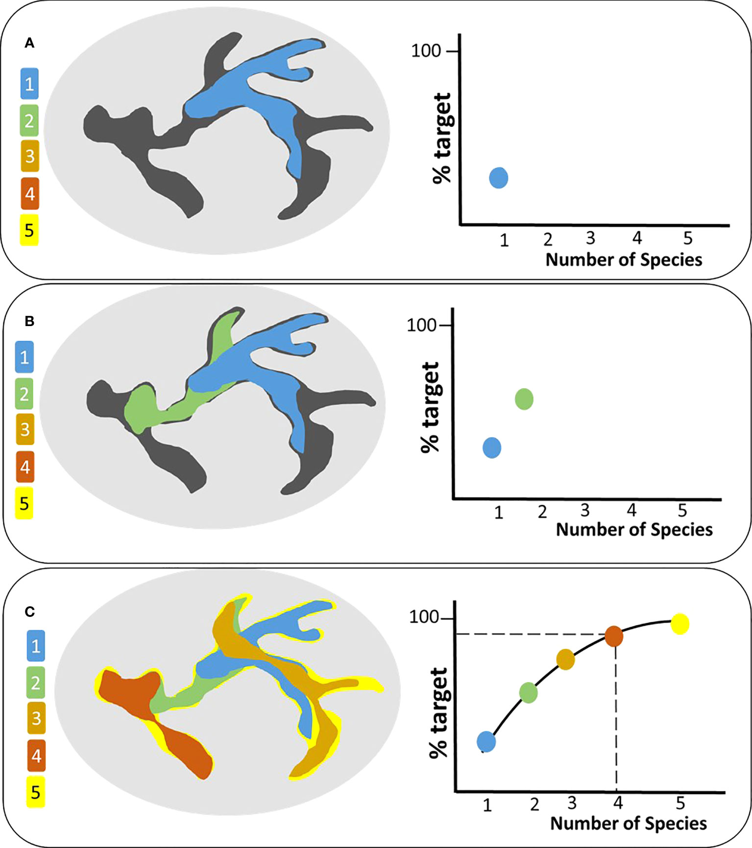
Figure 1 Conceptual figure of the selection process for connectivity umbrellas. The oval represents the region of analysis; the dark gray polygon represents the connectivity target. Five hypothetical species are shown in different colors and arranged according to their overall rank. Species are then added sequentially while quantifying their contribution towards the connectivity target (A–C) until an asymptote is reached. In this example, four species (blue, green, orange, maroon) are required to cover 95% of the target [dashed line in (C)].

The four main steps involved in this approach are: (1) Modelling connectivity for each species, (2) Generating connectivity targets per region, (3) Ranking species in each region, and finally (4) Determining the suite of umbrella species.

2.1 Step 1. Modelling connectivity for each species

We modelled connectivity between Protected Areas (PAs) within the suitable habitat for all large terrestrial mammals in Europe. We first selected species for the analysis, identified PAs to be used as nodes for connectivity analysis for each species, generated species-specific resistance surfaces that represented the potential difficulty of movement between nodes, and estimated potential connectivity for each species (Figure S1, Step 1).

2.1.1 Step 1a. Selecting species and traits for the study

We selected large terrestrial mammals, species with a mean body mass larger than 3 kg (Cardillo et al., 2005), that are native to Europe. We used the PanTHERIA database to obtain data on species traits (Jones et al., 2009) and putative maximum dispersal distances based on allometric scaling equations from previous studies (Santini et al., 2013; Whitmee and Orme, 2013). Details of the species used in this study are presented in Table S1.

2.1.2 Step 1b. Selecting nodes

Within the extent of occurrence and suitable habitat of each species (Maiorano et al., 2013), we selected PAs (IUCN Level I–IV) and Natura 2000 sites that reported presence of the species (European Environment Agency, 2020). We calculated the Euclidean distance between each pair of nodes and only retained pairs that were equal to or less than the putative maximum dispersal distance presented in Table S1. As a result, each species had a unique set of pairwise nodes.

2.1.3 Step 1c. Generating the resistance surface

We used previously published habitat suitability maps of mammals in Europe (Maiorano et al., 2013), which were generated from three environmental variables – land cover, elevation, and distance to water. The habitat suitability models contained pixel values of 0, 1, 2 corresponding to non-habitat, marginal habitat, suitable habitat, respectively, for each species. Because animals are more tolerant of suboptimal habitat during dispersal (Mateo-Sánchez et al., 2015), we coded the suitability values as 0 (unsuitable) and 1 (suitable, where we pooled suitable and marginal habitats) and resampled each raster using a 3×3 moving window. For each of the 24 species, this step produced a continuous habitat suitability raster at 1 km resolution. We then converted this suitability surface to a landscape resistance raster, which represents the ability of an organism to cross a particular environment (Zeller et al., 2012).

Previous studies have found that resistance is often a non-linear negative exponential function of habitat suitability (Dudaniec et al., 2013; Mateo-Sánchez et al., 2015). Therefore, we converted habitat suitability surfaces using a negative exponential function (Balkenhol et al., 2020) derived from the following formula:

$$\text{R}=\text{CS}\times {100}^{(1-\text{HS)}}$$

where R is the resistance assigned to a specific cell, CS is the cell size in meters (here 1000 m) and HS is the habitat suitability associated with that cell. This conversion assumes that animals are more tolerant of suboptimal habitat and respond less strongly to low habitat suitability during dispersal. The final resistance values ranged from 1000–10,000 resistance units.

2.1.4 Step 1d: Corridor simulation

We mapped potential connectivity for each species using the stochastic modelling program LSCorridors (Ribeiro et al., 2017). LSCorridors uses the resistance surface to produce potential corridors between each pair of nodes by simulating multiple dispersal events. It then adds all pairwise maps to produce the overall connectivity map for the species, quantified as the Route Selection Frequency Index (RSFI), a measure of the probability that a particular pixel will be used by any dispersing individual. We conducted 50 simulations between each pair of nodes, without landscape influence (Measures by Pixel, MP method, scale = 1000m, variability = 2). With these settings, stochasticity between simulations is introduced by different starting and ending points within the nodes for each simulation and by the variability factor in the resistance map, which represents uncertainty in the values used to produce the resistance surface. We estimated potential connectivity between a total of 53023 pairs of nodes, which amounts to a total of 2,651,150 pairwise simulations.

At the end of all simulations for each species, we further pruned the pairwise simulations to retain only those PA-pairs that had a mean corridor length equal to or less than the maximum putative dispersal distance. Since the maximum RSFI values were different for each of the species, we normalized the final connectivity maps of the 24 mammals for further analyses. We conducted further analyses at two spatial scales as described below.

2.2 Step 2: Generating connectivity targets per region

Defining regions: We conducted analyses at two hierarchical levels based on ecoregion classifications within broad geographical regions in continental Europe. We combined the six biomes present in Europe (Olson et al., 2001) with the six broad geographic regions (excluding islands) which produced 13 geographic biomes, henceforth referred simply as biomes in this study. Nested within these 13 biomes there are a total of 36 ecoregions (eight biomes have 31 nested ecoregions while five biomes do not have ecoregions) (Figure S2).

Connectivity target: Our approach requires users to pre-define a spatially explicit connectivity target. We tested the impact of different connectivity targets based on three different conservation goals. The three targets are aimed at protecting connectivity networks for all species in the region (Target EQ), only high-quality connectivity networks (Target Q), or connectivity networks of conservation-concern species only (Target T) (Figure S1, Step 2). Details of how these targets were derived are explained here:

● Target EQ: This target represents the best quality corridor cells for all species equally. It is produced by first extracting high-quality corridor cells (top 25 percentile values for each species), and then summing the high-quality corridor cells for all species.

● Target Q: This target represents only the best quality corridor cells irrespective of which species are represented in the target. It is produced by first adding all the normalized species corridor maps into one composite raster, and then extracting the cells that contain the top 25 percentile values.

● Target T: This target represents all corridor cells used by species of conservation concern, which we defined as species endemic to Europe or with an IUCN red list status of Near Threatened or higher (Table S1). In Europe, these species are Lynx pardinus, Bison bonasus, Gulo gulo, Marmota marmota, Rupicapra pyrenaica, Capra ibex, and Capra pyrenaica. This target is produced by adding corridor cells of all conservation-concern species in any given region. Because nine of the 13 biomes contain species of conservation concern, this target existed only in nine biomes.

We chose target EQ to demonstrate our data-driven approach to select connectivity umbrella species as we believe most conservation actions would be concerned about several species in the region, rather than just high-quality regions (target Q) or only species of conservation concern (target T). We compared connectivity umbrellas selected for target EQ with target Q and T to test the sensitivity of our approach and results are presented in Figure S3.

2.3 Step 3: Ranking species

To rank the species in each region, we calculated an umbrella score “Uir”, which quantifies the suitability of each species as a connectivity umbrella. For each region, we used the connectivity maps of each species, wherein the normalized RSFI value represents the probability of connectivity of each cell for that species and a set of five criteria using the calculation:

$$Uir\sim N,A,F,S,P$$

U is the overall umbrella score for species i in region r, calculated as the product of five criteria listed below:

N is the total number of species present in the region r whose corridors overlap with that of species i, calculated as the total number of overlapping species (Figure S1, Step 3a).

FIGURE 2

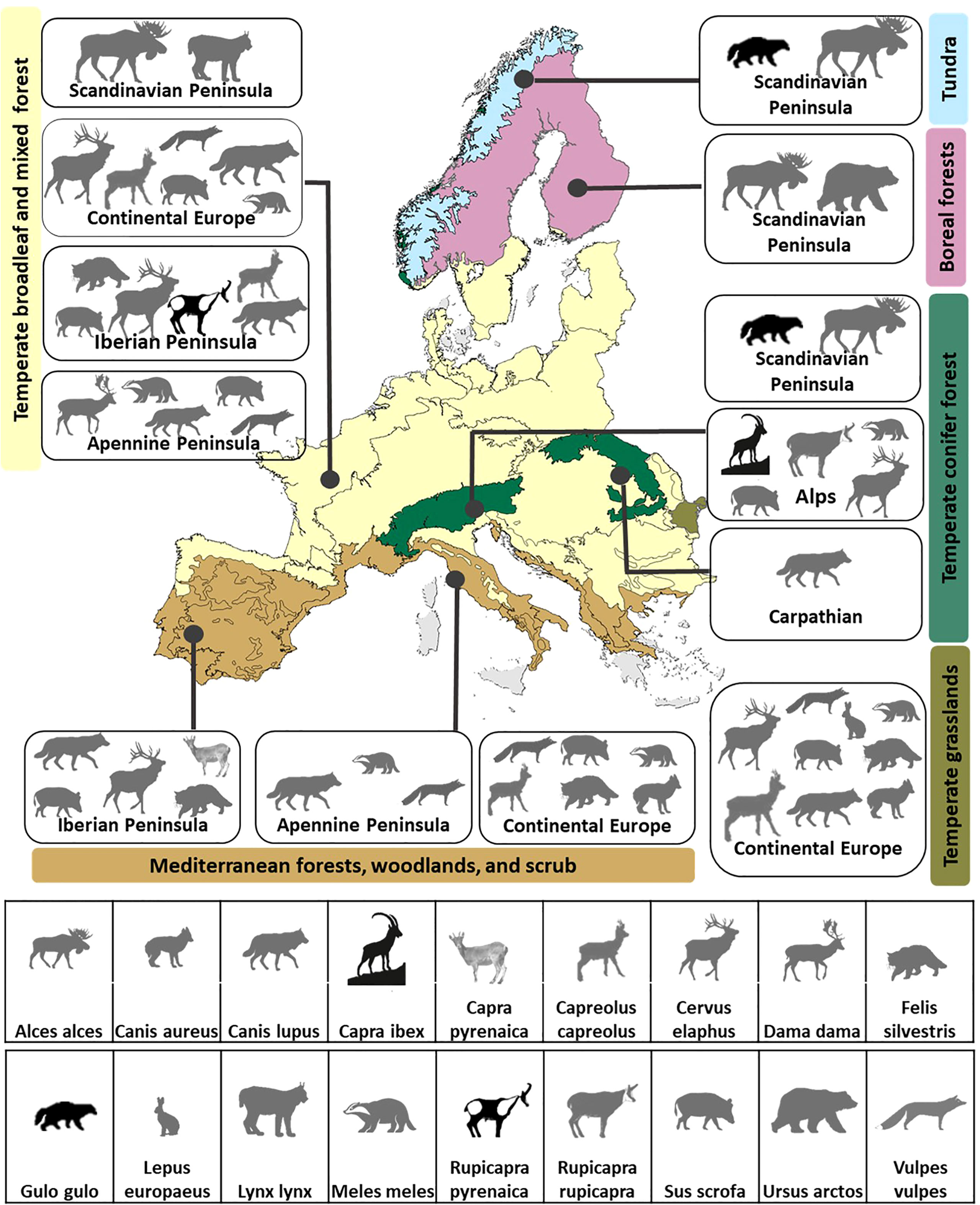
Figure 2 Connectivity umbrella species selected to reach 95% of the connectivity target in the thirteen biomes within major geographic regions in Europe. Species of conservation concern in Europe-wide assessments are represented by black silhouettes, all other species are represented by gray silhouettes.

A is the mean area of overlapping corridors of species i with all species corridors present in region r, calculated as the mean area (km²) of pairwise overlap of species i with all other species (Figure S1, Step 3b).

F is the fraction of the connectivity target in region r covered by species i, calculated as the percent area of intersection between the connectivity target and the corridor network of species i (Figure S1, Step 3c).

S is the mean strength of pairwise overlapping corridors, calculated as the mean of Bhattacharyya’s affinity index (Bhattacharya, 1943) that measures volumetric intersection of each pair of species (Fieberg and Kochanny, 2005). Bhattacharyya’s affinity index is a statistical measure of affinity between two populations that assumes they use space independently of one another. Values range from zero (no overlap) to 1 (complete overlap) (Figures S1, Step 3d).

P is the proportion of the total connectivity network of species i that lies within the connectivity target of region r, calculated as the sum of all pixel values within region r (Figure S1, Step 3e).

Criteria N (number of overlapping species), A (overlapping area with other species), F (fraction of target covered by the species) characterize the numerical suitability of a species at representing other species and the target. Criteria S (strength of overlapping corridors) and P (proportion of the species corridors within target) characterize the quality of a species at representing co-occurring species corridors and the target. Combining these criteria effectively select species that are representative of co-occurring species and the region under consideration (Figure S1, Step 3e).

2.4 Step 4: Determining the suite of umbrella species

Within each region, we ranked each species by its Uir value so that the species with the highest value received the highest rank. Effectively, this means that species with the highest ranks are those that overlapped with many other species, and did so over a larger area, with the highest strength of overlap, represented a large part of the connectivity network, and had a large part of their connectivity network within the region of interest. We plotted the species by their rank vs the additional contribution they made to the connectivity target. We first plotted the proportion of the connectivity target achieved by adding the corridors of the highest ranked species. We continued adding species according to their ranks, calculating the additional coverage of the connectivity target (that was not already covered by the previous species) for each species addition. We defined the suite of umbrella species as the number and combination of species required to cover at least 95% area of the connectivity target as adding more species beyond this asymptote did not make much improvement towards achieving the connectivity target (Figure S1, Step 4).

2.5 Evaluating the role of underlying landscape

Finally, to evaluate the role of landscape characteristics on the selection of connectivity umbrellas, we conducted a cluster analysis of all 36 ecoregions based on their mean human footprint, mean landscape fragmentation and the mean latitude. The human footprint index (Wildlife Conservation Society – WCS and Center for International Earth Science Information Network – CIESIN, Columbia University, 2005), generated from human population pressure, land use and infrastructure, and access, represents the cumulative anthropogenic impact on the environment, whereas the landscape fragmentation index (European Environment Agency, 2016) measured as the effective mesh density, i.e. landscape patches per 1000 km², represents a measure of the degree to which the landscape is fragmented. We performed agglomerative hierarchical cluster analysis on ecoregions to identify distinct clusters in our dataset. We used Ward’s method of agglomeration, which produces clusters of more equal size by keeping distances within the clusters as small as possible (Ward, 1963). We identified five unique groups using a dendrogram on the cluster solutions that we had obtained using the hclust function available with R library fastcluster (Müllner, 2013).

Within the clusters, we evaluated six attributes of connectivity umbrella species (mean body mass, home range size, population density, putative maximum dispersal distance, geographic range in Europe and conservation status (Table S1). We conducted Kruskal-Wallis tests to identify significant differences of attributes of connectivity umbrella species in the different clusters and used a post-hoc Dunns test to identify which clusters were significantly different using Holms-adjusted p-values to account for multiple comparisons.

3 Results

Using the approach presented in Figure 1, we demonstrate that a systematic and objective assessment of which and how many species are required to meet connectivity needs of multiple co-occurring species is indeed possible. In this process, we discovered some important patterns.

Multiple species are required to meet connectivity goals at both scales considered. Ninety-two percent of the biomes (Figure 2) and 83% of the ecoregions (Figure 3) had more than one connectivity umbrella species. Both the number and identity of species are scale dependent. More species are selected at the biome level (average 4.15, range 1–9 species; Figure 2) than at the ecoregion level (average 3.16, range 1–9 species; Figures 3A, S4). The identity of the species selected also varies across scales. For example, six species are selected in the temperate broadleaf mixed forest biome (Figure 3A), whereas several of the species selected in the eleven nested ecoregions (ranging from 1 to 6) are exclusive to the ecoregions, i.e., not selected in the biome-level analysis (Figure 3B).

FIGURE 3

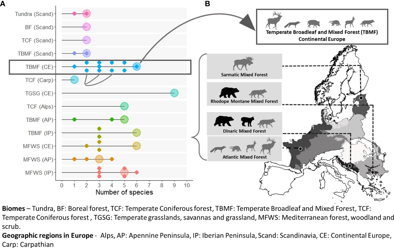
Figure 3 The number (A) and identity (B) of connectivity umbrella species vary across spatial scales. More species are selected at the broad biome level [represented by large dots in (A)] than at the finer ecoregion level [represented by smaller dots in (A)]. Biomes are represented by different colors. Connectivity umbrellas selected at finer scale often include unique and conservation-concern species [grey boxes in (B)], not selected at the coarse scale white box in (B). Species identified to be of conservation concern in ecoregional assessments are represented by black silhouettes.

Connectivity coverage achieved using single species is highly variable (Figure S5). For example, if only the highest-ranking species were to be selected, an average of 75% of the regional targets would be covered, ranging from ~14% by the Iberian lynx (Lynx pardinus) in Southwest Iberian Mediterranean sclerophyllous and mixed forests to ~97% by the wolf (Canis lupus) in South Apennine mixed montane forests. If only the highest-ranking species of conservation concern is selected, an average of 25% of the individual regional targets would be covered, ranging from ca. 1% by the bison in the Carpathian Mountains to 95% by the wolverine in the Scandinavian Tundra. Some ecoregions in the Scandinavian and Apennine peninsulas are exceptions to this general pattern.

Our results indicate that even when species of conservation concern are present in a region, they may not necessarily be the most suitable connectivity umbrellas. A total of seven conservation-concern species are present in 17 ecoregions (47% of ecoregions, average 1.3 conservation-concern species/region), but are selected as connectivity umbrellas in only 9 ecoregions (~53% where they are present). The number or proportion of conservation-concern species present in any region is not significantly correlated to the number or proportion of conservation-concern species in the suite of connectivity umbrella species (Pearson’s r = 0.04 and 0.26, respectively; p > 0.05 in both cases). We used Red List status at the European level because it was consistent with the European extent of our study, but threat assessments at regional scales may also be relevant. For example, none of the species selected as connectivity umbrellas in the temperate broadleaf mixed forest biome are of conservation concern at the European scale (Figure 3B), but the brown bear (Ursus arctos) and Eurasian lynx (Lynx lynx), selected at the ecoregion scale are categorized as vulnerable and endangered in the Rhodope and Dinaric Mountain ecoregions (Temple and Terry, 2007).

Of the 24 species evaluated, not even one species is an effective connectivity umbrella across its entire range (Figure 4). Even the species selected most often, the wolverine (Gulo gulo) and moose (Alces alces), were only selected as connectivity umbrellas in 60% of the regions in which they occur. While there is a significantly higher chance of being selected as an umbrella species for wider ranging species, i.e., species that occur in many regions (Pearson’s r = 0.73, p<.05), this effect is lost when comparing the occurrence of species across multiple ecoregions with the proportion of the times that it is selected as a connectivity umbrella (Pearson’s r = 0.13, p = 0.66).

FIGURE 4

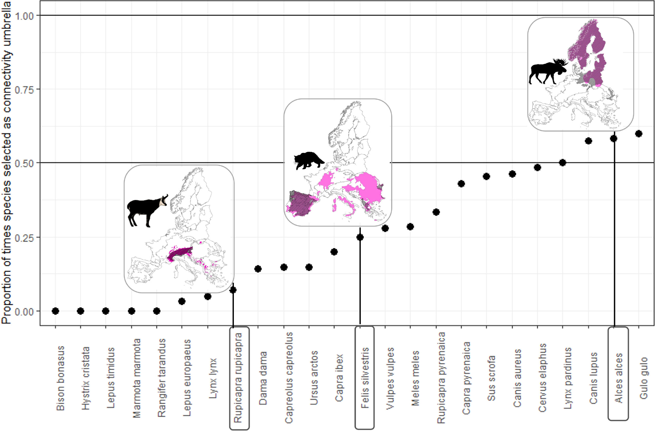
Figure 4 No species is selected as a connectivity umbrella everywhere it occurs. For each species in the x-axis, the y-axis represents the number of times it was selected as a connectivity umbrella everywhere it is present. For example, the distribution ranges of the moose (Alces alces), wildcat (Felis silvestris), and chamois (Rupicapra rupicapra) are shown in pink, and the ecoregions where they are selected as connectivity umbrellas are shown in hashed lines.

We identified five unique clusters of ecoregions that ranged from very low to very high human influence (Figure S6). Mountain ranges and regions at higher latitudes are generally less fragmented and impacted by humans than regions in the plains or at lower latitudes. The maximum dispersal distance (Kruskal-Wallis chi-squared = 10.942, df = 4, p-value = 0.027), home range (chi-squared = 12.401, df = 4, p-value = 0.014), proportion of range in Europe (chi-squared = 21.014, df = 4, p-value = 0.0003), and conservation status (chi-squared = 9.9392, df = 4, p-value = 0.041) of connectivity umbrella species are significantly different between the clusters. On average, species selected as connectivity umbrellas in regions with low human influence have higher mean body mass, larger home ranges, longer dispersal distances, smaller geographic ranges, occur at lower population densities, and are of higher conservation concern than connectivity umbrellas in more human-influenced regions (Figures 5A–F). Proportionally more species are required to meet connectivity targets in regions with high human influence (Figure 5G).

FIGURE 5

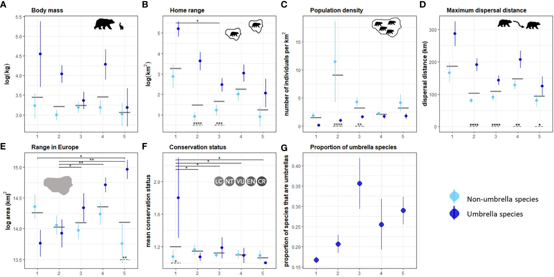
Figure 5 Attributes of species across clusters arranged from lowest (1) to highest (5) human impact. The means and standard errors of attributes of connectivity umbrellas (dark blue) and non-umbrellas (light blue) are shown in (A–F), along with the mean attribute value in the cluster as a grey bar. The proportion of species selected as connectivity umbrellas in each cluster is shown in (G). Significant difference of mean values between clusters are shown on the top in solid lines and between umbrella and non-umbrella species within clusters are shown at the bottom in panels (A–F). * indicates a p-value ≤ 0.05, ** a p-value ≤ 0.01, and *** a p-value ≤ 0.001.

4 Discussion

Our approach increases objectivity when selecting umbrella species for connectivity conservation. It can be applied to multiple-taxonomic groups and to varying spatial scales. Unlike static target-setting in conservation prioritization exercises, our approach is flexible and can be adapted to test which species would suit different conservation goals and scenarios.

Two methods have been developed to specifically select species-based surrogates for connectivity planning. Lechner et al. (2017) use a cluster analysis on habitat requirements, connectivity elements, and gap-crossing distance thresholds to group twelve candidate mammal species into five distinct dispersal guilds. Connectivity for each guild is then modelled separately to identify which guild of species are more sensitive to habitat fragmentation. Meurant et al. (2018) present an approach to select multi-taxa surrogates from a pool of candidate species that represent a diversity of habitat needs and movement abilities. From a set of fourteen candidate species, the authors create a reference spatial prioritization map and run multiple permutations and combinations of the fourteen candidate species to identify the species subset that best retains different thresholds of the reference spatial priority map. Our approach is different from both methods. First, we include the entire terrestrial large mammal community in Europe without going through a pre-selection process as in Meurant et al. (2018), where they selected fourteen candidate species from a pool of 48 mammals, 216 birds, and 32 amphibians and reptiles based on a previous study (Albert et al., 2017). Second, we do not group species into dispersal guilds, diversity of habitat, or movement requirements. We treat each species independently. Further, instead of using a conservation concern filter in selecting the species to include in the candidate pool, we use the results to guide and test how frequently species of conservation concern are suitable connectivity umbrellas. Finally, in addition to addressing which and how many species are required for connectivity planning, we also evaluate the species-surrogates approach across two different geographic scales and assess the characteristics of connectivity umbrellas in landscapes with varying levels of human influence.

Our results re-confirm previous findings on the fine-filter surrogate approach that multiple species are better than any single surrogate species (Meurant et al., 2018; Wang et al., 2018) and a priori selection of certain groups, e.g., carnivores, may not be suitable connectivity umbrellas (Beier et al., 2009). Most suites of species selected in our analyses consist of a combination of herbivores and carnivores. Such mixed suites of species have diverse ecological attributes and dispersal abilities and are therefore more likely to accommodate the ecological requirements of diverse terrestrial mammal communities and their differing sensitivities to environmental conditions. In addition to corroborating previous findings, we show that both the number and the identity of species differ by the scale of analysis, and that species selected at finer scales are not subsets of those selected at broader scales (Figure 3).

Our approach is flexible in two ways. First, the result is a suite of species that are needed to cover 95% of the connectivity target. Depending on the regional context, it is possible to sub-select from within this suite of species, especially when species provide very little percent improvement towards the overall target. Second, the evaluation of sensitivity to different connectivity targets (Figure S3) provides a way to select species that are suitable for a diversity of conservation goals. For example, moose and wolverine in the northern regions, red deer (Cervus elaphus) and Iberian Ibex (Capra pyrenaica) in the Mediterranean forests, woodland and scrub of the Iberian Peninsula and wolf in the Apennine peninsula, red deer and red fox (Vulpes vulpes) in temperate broadleaf and mixed forest in central Europe, and the Alpine ibex in the Alps, are species selected in all three connectivity targets which were created with very different conservation goals. In general, target EQ required more species than target Q or T. This is intuitive because target EQ represents all species, target Q represents only high-quality corridors irrespective of species, and target T only represents species of conservation concern. The identity of species selected across the targets changed in their rank, but in general the top-ranking species were consistent across the different targets, and the pool of species that was most highly ranked remained similar. This redundancy in the selection of species across disparate conservation goals can be a valuable tool to incorporate more certainty about including a particular species to be an umbrella for connectivity conservation.

An important finding is the interaction between the attributes of landscape and species selected as connectivity umbrellas. The interaction between species and landscape indicates that species selected to be surrogates for connectivity conservation need to be tailored to the level of human influence in the landscape under consideration. To be effective in highly humanized landscapes, numerically more species with a certain set of attributes (widely distributed but smaller-bodied species that occur at higher population densities and disperse over shorter distances) may be required. These attributes are generally not associated with umbrella species but may be the key to developing region-specific effective connectivity plans.

The aim of our study is not to prescribe which species should be used for connectivity conservation in Europe. Rather, we use continental Europe as an example to demonstrate an approach that is quite flexible and can accommodate many different conservation and modelling choices. Due to the continental scale of analyses, we use several simplifications in our modelling to optimize computational time. We used coarse-scale (1 km) existing habitat suitability maps to generate resistance surfaces and model connectivity between PAs, but it is noteworthy that source populations may also be present in habitat patches outside of the PA network, and individual species are likely to be impacted by more and different sets of variables. Therefore, we caution the use of the species presented here to be effective and “correct” connectivity umbrellas. The species presented here can be starting points, but we recommend users to create resistance surfaces using variables and resolutions that are relevant to their region of interest. It will most likely be computationally plausible to run regional models using non-protected habitat patches as source populations at a finer resolution and include more variables to develop more realistic resistance surfaces.

Our approach can easily be extended to other systems not presented here. For example, we analyze only terrestrial mammals, but other taxonomic groups of interest can easily be used to conduct similar analyses. We define three different connectivity targets based on different conservation goals, but connectivity targets may be defined in many other ways. Finally, we use a threshold of 95% of the target as our goal (guided by our observation that an asymptote is reached around 95%), but users may decide to use a different threshold. Our approach should be applicable in any focal landscape where it is possible to generate a connectivity network for multiple species.

Overall, we demonstrate that an objective selection of surrogate species for connectivity planning is possible. Considering multiple species, not just in relation to species attributes but in relation to landscape scale and characteristics may be the key towards identifying connectivity umbrellas that better represent the needs of entire species communities. In practice, decision-making in conservation is a complex process, involving many stakeholders, and is highly contextual. When species are tied in rank and contribution to the connectivity target, managers or conservationists could select species with a higher social acceptance or other issues that are relevant locally or regionally. Rather than advocating for one species over another, we present an approach to remove the guesswork over which species should be selected as connectivity umbrellas and increase objectivity in the selection of multispecies conservation strategies.

Conservation targets, whether modest at 30% of terrestrial land (CBD, 2023), or ambitious at 50% (Dinerstein et al., 2017), are unachievable without integrating connectivity conservation, especially in rapidly changing ecosystems in the Anthropocene. The key to selecting umbrella species for connectivity conservation is to move beyond arbitrary selection of species, for the selection process to be objective, and in relation to the scale and attributes of the landscape. Only then can the overall goal of connectivity conservation be realized and be effective in restoring ecosystems and decreasing biodiversity loss.

Data availability statement

The original contributions presented in the study are publicly available. This data can be found here: https://figshare.com/s/23831fdc52a9dcc60a36.

Author contributions

TD, NB, and MDB contributed to conception and design of the study. JS contributed towards the analyses and SF’s contributions helped improve the figures. TD wrote the first draft of the manuscript. All authors contributed to the article and approved the submitted version.

Funding

This research is part of project BearConnect, funded through the 2015–2016 BiodivERsA COFUND call, with national funders Agence Nationale de la Recherche (ANR), France (Grant number: ANR-16-EBI3-0003), National Science Center (NCN), Poland (Grant number: 2016/22/Z/NZ8/00121), Federal Ministry of Education and Research (BMBF) and DLR Project Management Agency (DLR-PT), Germany (Grant number: 01LC1614A), Romanian National Authority for Scientific Research and Innovation, CCCDI – UEFISCDI, Romania (Grant number: BiodivERsA3-2015-147-BearConnect (96/2016) within PNCDI III, and Norwegian Research Council (RCN), Norway (Grant number: 269863).

Acknowledgments

We thank Phylopic and all the creators who provided animal silhouettes in the public domain which we used in the different figures in this paper. We would like to thank Drs. Fanie Pelletier, Moreno Di Marco, Thomas Mueller, Ninon Meyer, and Nina Gerber for their reviews on previous versions of this manuscript. We acknowledge support by the Open Access Publication Funds of the University of Goettingen.

Conflict of interest

Author MDB is a founder of DivjaLabs Ltd.

The remaining authors declare that the research was conducted in the absence of any commercial or financial relationships that could be construed as a potential conflict of interest.

Publisher’s note

All claims expressed in this article are solely those of the authors and do not necessarily represent those of their affiliated organizations, or those of the publisher, the editors and the reviewers. Any product that may be evaluated in this article, or claim that may be made by its manufacturer, is not guaranteed or endorsed by the publisher.

Supplementary material

The Supplementary Material for this article can be found online at: https://www.frontiersin.org/articles/10.3389/fevo.2023.1078649/full#supplementary-material

References

Albert C. H., Rayfield B., Dumitru M., Gonzalez A. (2017). Applying network theory to prioritize multi-species habitat networks that are robust to climate and land-use change. Conserv. Biol. 31, 1383–1396. doi: 10.1111/cobi.12943

PubMed Abstract | CrossRef Full Text | Google Scholar

Balkenhol N., Schwartz M. K., Inman R. M., Copeland J. P., Squires J. S., Anderson N. J., et al. (2020). Landscape genetics of wolverines (Gulo gulo): scale-dependent effects of bioclimatic, topographic, and anthropogenic variables. J. Mammal. 101, 790–803. doi: 10.1093/jmammal/gyaa037

PubMed Abstract | CrossRef Full Text | Google Scholar

Beier P., Majka D. R., Newell S. L. (2009). Uncertainty analysis of least-cost modeling for designing wildlife linkages. Ecol. Appl. 19, 2067–2077. doi: 10.1890/08-1898.1

PubMed Abstract | CrossRef Full Text | Google Scholar

Belote R. T., Dietz M. S., Jenkins C. N., McKinley P. S., Irwin G. H., Fullman T. J., et al. (2017). Wild, connected, and diverse: building a more resilient system of protected areas. Ecol. Appl. 27, 1050–1056. doi: 10.1002/eap.1527

PubMed Abstract | CrossRef Full Text | Google Scholar

Bhattacharya A. (1943). On a measure of divergence between two statistical populations defined by their probability distributions. Bull. Calcutta Math. Soc 35, 99–109.

Google Scholar

Boyd C., Brooks T. M., Butchart S. H. M., Edgar G. J., Fonseca G. A. B. D., Hawkins F., et al. (2008). Spatial scale and the conservation of threatened species. Conserv. Lett. 1, 37–43. doi: 10.1111/j.1755-263X.2008.00002.x

CrossRef Full Text | Google Scholar

Brodie J. F., Giordano A. J., Dickson B., Hebblewhite M., Bernard H., Mohd-Azlan J., et al. (2015). Evaluating multispecies landscape connectivity in a threatened tropical mammal community. Conserv. Biol. 29, 122–132. doi: 10.1111/cobi.12337

PubMed Abstract | CrossRef Full Text | Google Scholar

Brost B. M., Beier P. (2012). Use of land facets to design linkages for climate change. Ecol. Appl. 22, 87–103. doi: 10.1890/11-0213.1

PubMed Abstract | CrossRef Full Text | Google Scholar

Cardillo M., Mace G. M., Jones K. E., Bielby J., Bininda-Emonds O. R. P., Sechrest W., et al. (2005). Multiple causes of high extinction risk in large mammal species. Science 309, 1239–1241. doi: 10.1126/science.1116030

PubMed Abstract | CrossRef Full Text | Google Scholar

Caro T. M., Girling S. (2010). Conservation by proxy: indicator, umbrella, keystone, flagship, and other surrogate species (Washington, DC: Island Press).

Google Scholar

Caro T. M., O’Doherty G. (1999). On the use of surrogate species in conservation biology. Conserv. Biol. 13, 805–814. doi: 10.1046/j.1523-1739.1999.98338.x

CrossRef Full Text | Google Scholar

CBD (2010). “Strategic plan for biodiversity 2011–2020 and the aichi targets,” in Report of the Tenth Meeting of the Conference of the Parties to the Convention on Biological Diversity. Nagoya, Japan. Available at: https://wedocs.unep.org/20.500.11822/27533.

Google Scholar

CBD (2020). Update of the zero draft of the post-2020 global biodiversity framework (Convention on biological diversity). Available at: https://www.cbd.int/doc/c/3064/749a/0f65ac7f9def86707f4eaefa/post2020-prep-02-01-en.pdf (Accessed June 14, 2023)

Google Scholar

CBD (2023) 2030 targets and guidance notes. secretariat of the convention on biological diversity. Available at: https://www.cbd.int/gbf/targets/ (Accessed June 14, 2023).

Google Scholar

Ceballos G., Ehrlich P. R., Dirzo R. (2017). Biological annihilation via the ongoing sixth mass extinction signaled by vertebrate population losses and declines. Proc. Natl. Acad. Sci. 114, E6089–E6096. doi: 10.1073/pnas.1704949114

CrossRef Full Text | Google Scholar

Chase J. M., Blowes S. A., Knight T. M., Gerstner K., May F. (2020). Ecosystem decay exacerbates biodiversity loss with habitat loss. Nature. 584, 238–243. doi: 10.1038/s41586-020-2531-2

PubMed Abstract | CrossRef Full Text | Google Scholar

Crooks K. R., Burdett C. L., Theobald D. M., King S. R. B., Di Marco M., Rondinini C., et al. (2017). Quantification of habitat fragmentation reveals extinction risk in terrestrial mammals. Proc. Natl. Acad. Sci. 114, 7635–7640. doi: 10.1073/pnas.1705769114

CrossRef Full Text | Google Scholar

Cushman S. A., Landguth E. L. (2012). Multi-taxa population connectivity in the northern rocky mountains. Ecol. Model. 231, 101–112. doi: 10.1016/j.ecolmodel.2012.02.011

CrossRef Full Text | Google Scholar

Dinerstein E., Olson D., Joshi A., Vynne C., Burgess N. D., Wikramanayake E., et al. (2017). An ecoregion-based approach to protecting half the terrestrial realm. BioScience 67, 534–545. doi: 10.1093/biosci/bix014

PubMed Abstract | CrossRef Full Text | Google Scholar

Dudaniec R. Y., Rhodes J. R., Worthington Wilmer J., Lyons M., Lee K. E., McAlpine C. A., et al. (2013). Using multilevel models to identify drivers of landscape-genetic structure among management areas. Mol. Ecol. 22, 3752–3765. doi: 10.1111/mec.12359

PubMed Abstract | CrossRef Full Text | Google Scholar

European Commission (2020) EU Biodiversity strategy for 2030. bringing nature back into our lives. communication from the commission to the European parliament, the council, the European economic and social committee and the committee of the regions. Available at: https://ec.europa.eu/environment/nature/biodiversity/strategy/index_en.htm (Accessed May 23, 2020).

Google Scholar

European Environment Agency (2016) Landscape fragmentation indicator effective mesh density (seff) - major and medium anthropogenic fragmentation (FGA2_S_2016). Available at: https://www.eea.europa.eu/data-and-maps/data/landscape-fragmentation-indicator-effective-mesh (Accessed July 21, 2020).

Google Scholar

European Environment Agency (2020) Natura 2000 data - the European network of protected sites [[/amp]]mdash; European environment agency. Available at: https://www.eea.europa.eu/data-and-maps/data/natura-11 (Accessed January 25, 2020).

Google Scholar

Fieberg J., Kochanny C. O. (2005). Quantifying home-range overlap: the importance of the utilization distribution. J. Wildl. Manage. 69, 1346–1359. doi: 10.2193/0022-541X(2005)69[1346:QHOTIO]2.0.CO;2

CrossRef Full Text | Google Scholar

Gilpin M. E., Soulé M. E. (1986). “Minimum viable populations: processes of species extinction,” in Conservation biology: the science of scarcity and diversity. Ed. Soulé M. E. (Sunderland, MA: Sinauer Associates), 19–34.

Google Scholar

Jones K. E., Bielby J., Cardillo M., Fritz S. A., O’Dell J., Orme C. D. L., et al. (2009). PanTHERIA: a species-level database of life history, ecology, and geography of extant and recently extinct mammals. Ecology 90, 2648–2648. doi: 10.1890/08-1494.1

CrossRef Full Text | Google Scholar

Krosby M., Breckheimer I., John Pierce D., Singleton P. H., Hall S. A., Halupka K. C., et al. (2015). Focal species and landscape “naturalness” corridor models offer complementary approaches for connectivity conservation planning. Landsc. Ecol. 30, 2121–2132. doi: 10.1007/s10980-015-0235-z

CrossRef Full Text | Google Scholar

Lechner A. M., Sprod D., Carter O., Lefroy E. C. (2017). Characterising landscape connectivity for conservation planning using a dispersal guild approach. Landsc. Ecol. 32, 99–113. doi: 10.1007/s10980-016-0431-5

CrossRef Full Text | Google Scholar

Maiorano L., Amori G., Capula M., Falcucci A., Masi M., Montemaggiori A., et al. (2013). Threats from climate change to terrestrial vertebrate hotspots in Europe. PloS One 8. doi: 10.1371/journal.pone.0074989

CrossRef Full Text | Google Scholar

Mateo-Sánchez M. C., Balkenhol N., Cushman S., Pérez T., Domínguez A., Saura S. (2015). Estimating effective landscape distances and movement corridors: comparison of habitat and genetic data. Ecosphere 6, 1–16. doi: 10.1890/ES14-00387.1

CrossRef Full Text | Google Scholar

Meurant M., Gonzalez A., Doxa A., Albert C. H. (2018). Selecting surrogate species for connectivity conservation. Biol. Conserv. 227, 326–334. doi: 10.1016/j.biocon.2018.09.028

CrossRef Full Text | Google Scholar

Mitchell M. G., Bennett E. M., Gonzalez A. (2013). Linking landscape connectivity and ecosystem service provision: current knowledge and research gaps. Ecosystems 16, 894–908. doi: 10.1007/s10021-013-9647-2

CrossRef Full Text | Google Scholar

Müllner D. (2013). Fastcluster: fast hierarchical, agglomerative clustering routines for r and Python. J. Stat. Software 53, 1–18. doi: 10.18637/jss.v053.i09

CrossRef Full Text | Google Scholar

Olson D. M., Dinerstein E., Wikramanayake E. D., Burgess N. D., Powell G. V. N., Underwood E. C., et al. (2001). Terrestrial ecoregions of the world: a new map of life on earth. BioScience 51, 933–938. doi: 10.1641/0006-3568(2001)051[0933:TEOTWA]2.0.CO;2

CrossRef Full Text | Google Scholar

Ribeiro J. W., Silveira dos Santos J., Dodonov P., Martello F., Brandão Niebuhr B., Ribeiro M. C. (2017). LandScape corridors (lscorridors): a new software package for modelling ecological corridors based on landscape patterns and species requirements. Methods Ecol. Evol. 8, 1425–1432. doi: 10.1111/2041-210X.12750

PubMed Abstract | CrossRef Full Text | Google Scholar

Robillard C. M., Coristine L. E., Soares R. N., Kerr J. T. (2015). Facilitating climate-change-induced range shifts across continental land-use barriers. Conserv. Biol. 29, 1586–1595. doi: 10.1111/cobi.12556

CrossRef Full Text | Google Scholar

Santini L., Marco M. D., Visconti P., Baisero D., Boitani L., Rondinini C. (2013). Ecological correlates of dispersal distance in terrestrial mammals. Hystrix Ital. J. Mammal. 24, 181–186. doi: 10.4404/hystrix-24.2-8746

CrossRef Full Text | Google Scholar

Temple H. J., Terry A. (Compilers) (2007). The status and distribution of European mammals. (Luxembourg: Office for Official Publications of the European Communities).. Available at: https://portals.iucn.org/library/sites/library/files/documents/RL-4-013.pdf (Accessed July 18, 2020).

Google Scholar

Theobald D. M., Reed S. E., Fields K., Soulé M. (2012). Connecting natural landscapes using a landscape permeability model to prioritize conservation activities in the united states: connecting natural landscapes. Conserv. Lett. 5, 123–133. doi: 10.1111/j.1755-263X.2011.00218.x

CrossRef Full Text | Google Scholar

Wang F., McShea W. J., Li S., Wang D. (2018). Does one size fit all? a multispecies approach to regional landscape corridor planning. Divers. Distrib. 24, 415–425. doi: 10.1111/ddi.12692

CrossRef Full Text | Google Scholar

Ward J. H. (1963). Hierarchical grouping to optimize an objective function. J. Am. Stat. Assoc. 58, 236–244. doi: 10.1080/01621459.1963.10500845

PubMed Abstract | CrossRef Full Text | Google Scholar

Whitmee S., Orme C. D. L. (2013). Predicting dispersal distance in mammals: a trait-based approach. J. Anim. Ecol. 82, 211–221. doi: 10.1111/j.1365-2656.2012.02030.x

CrossRef Full Text | Google Scholar

Wiens J. A., Hayward G. D., Holthausen R. S., Wisdom M. J. (2008). Using surrogate species and groups for conservation planning and management. BioScience 58, 241–252. doi: 10.1641/B580310

CrossRef Full Text | Google Scholar

Wildlife Conservation Society-WCS, Center for International Earth Science Information Network-CIESIN-Columbia University (2005). Last of the wild project, version 2, 2005 (LWP-2): global human footprint dataset (Geographic). Palisades, New York: NASA Socioeconomic Data and Applications Center (SEDAC). doi: 10.7927/H4M61H5F. Accessed May 23, 2020.

CrossRef Full Text | Google Scholar

Wood S. L. R., Martins K. T., Dumais-Lalonde V., Tanguy O., Maure F., St-Denis A., et al. (2022). Missing interactions: the current state of multispecies connectivity analysis. Front. Ecol. Evol. 10. doi: 10.3389/fevo.2022.830822

CrossRef Full Text | Google Scholar

Zeller K. A., McGarigal K., Whiteley A. R. (2012). Estimating landscape resistance to movement: a review. Landscape Ecology 27, 777–797. doi: 10.1007/s10980-012-9737-0

CrossRef Full Text | Google Scholar