Coco: conservation design for optimal ecological connectivity

1 Introduction

Biodiversity loss is one of the biggest problems we currently face, with many species threatened by extinction. Climate change and other anthropogenic environmental impacts exacerbate the degradation of ecosystems and the decline of biodiversity (Rands et al., 2010). Even with broad public support and an increasing number of policies and actions for biodiversity conservation, biodiversity continued to decline between 2011 and 2020 (Lucy, 2022). Around 1 million species face extinction in the coming decades unless the drivers of biodiversity loss are reduced (IPBES, 2019). However, indicators show an increase in main drivers responsible for biodiversity loss, i.e., habitat fragmentation due to land-use change and climate change (Rands et al., 2010). Habitat fragmentation has a detrimental impact on biodiversity and ecological processes (Haddad et al., 2015); both island biogeography (Newmark, 1987) and metapopulation theory (Hanski et al., 1999) suggest that isolation increases the risk of species extinction. Additionally, the global average temperature increase of 1°C has a disastrous impact on ecosystems, making minimization of this impact of climate change on ecological processes key (Scheffers et al., 2016). Because of climate change, many species are shifting range boundaries and will continue to do so (Littlefield et al., 2019).

To maintain higher biodiversity over time, large, connected conservation areas, e.g., protected areas and other effective area-based conservation measures, are needed (Hilty et al., 2020) and should be expanded to cover at least 30% of the planet by 2030 (Lucy, 2022). These conservation areas form a buffer between species and the drivers that threaten their survival. They should represent the complete variety of biodiversity and promote the long-term survival of the protected species (Margules and Pressey, 2000).

Thus, conservation design should take ecological connectivity into account, in addition to natural, physical and biological patterns. Due to the importance of the connectivity of the landscape for biodiversity conservation, the study of ecological connectivity has steadily grown in recent years (Ayram et al., 2016). Ecological connectivity defines the extent to which the landscape facilitates or impedes the movement of animals and plants (Crooks and Sanjayan, 2006). Conserving connectivity improves the flow of organisms, materials, energy, and information across landscapes. It facilitates the integrity and functionality of ecosystems and the maintenance of biodiversity and ecosystem services (Crooks and Sanjayan, 2006) and is fundamental to species persistence by accommodating species to avoid anthropogenic threats (Cushman et al., 2013).

Protecting and restoring ecological connectivity can mitigate some of the effects of land-use change (Arkilanian et al., 2020) and improve migration, natural adaptation and persistence of species under climate change (Heller and Zavaleta, 2009). Thus, ensuring the permeability and traversability of the landscape enables climate and land-use driven range shifts (Keeley et al., 2018; Tucker et al., 2018). Conservation areas are predominantly natural areas with high biodiversity content (Keeley et al., 2018), mainly designed to conserve biodiversity. However, ecological connectivity has an increasing role in their design. Ecological corridors are geographical spaces solely designated to maintain or restore ecological connectivity (Hilty et al., 2020). Ecological networks consist of conservation areas and ecological corridors designed, implemented and maintained to restore, conserve or enhance biodiversity (Bennett, 2004; Bennett and Mulongoy, 2006; Hilty et al., 2020). Many modelling approaches exist to help balance the many factors influencing conservation planning. These approaches regularly focus on habitat networks for single species (Ayram et al., 2016; Xue et al., 2017; Gupta et al., 2019). In contrast, there is broad consensus for the need for approaches that assess connectivity for multiple co-habiting species in the landscape. Multispecies connectivity analysis aims to identify a network of habitats and movement pathways that supports the long-term persistence of multiple species in a landscape (Wood et al., 2022). There are different methods to integrate multiple species into conservation design.

Conservation design aims to provide biodiversity and habitat conservation in response to altered climates and land-use change (Groves et al., 2012). Its tasks are to identify where to achieve conservation goals, which locations to prioritize and how to implement conservation actions (Redford et al., 2003; Wilson et al., 2007). Conservation frameworks offer guidance for the planning and management of these conservation efforts. There are multiple general conservation frameworks, such as Strategic Foresight (Cook et al., 2014), Evidence-Based Practice (EBP) (Sutherland, 2008) and Systematic Conservation Planning (SCP) (Margules and Pressey, 2000), each with specialized core focal problems (Schwartz et al., 2018). Each framework contains a set of tools and guidelines, such as Decion Support Systems (DSSs) that aid in addressing the focal problem of the framework (Schwartz et al., 2018). DSSs are usually applied to advise planners, managers and stakeholders. Widely used DSSs being applied globally (Rose et al., 2021) include Conservation Evidence (Sutherland et al., 2019), a tool that summarizes documented evidence for EBP, TESSA (Peh et al., 2013), a policy support tool to guide the appraisal of ecosystem services at individual sites and the Ecosystem Management Decision Support system (Reynolds et al., 2014), a knowledge-based decision support system for ecological planning and analysis, widely applied to landscape analysis in the US (Gibson et al., 2017). Marxan (Ball et al., 2009) is claimed to be the most widely used DSS globally (Gibson et al., 2017). It is a spatial planning tool for SCP that identifies subsets of the conservation planning area that achieve the conservation goals while taking tradeoffs between conservation and socio-economic objectives into account.

Here, we concentrate on spatial planning in the SCP framework. In more detail, SCP provides a general framework for locating and designing conservation areas. It consists of the following six stages with many feedback loops and revisions about the selected conservation area: compile data on biodiversity, identify conservation goals, review existing conservation areas, select additional conservation areas, implement conservation actions, and maintain the conservation area (Margules and Pressey, 2000; Gaston et al., 2002). The purpose of selecting additional conservation areas is to achieve the conservation goals subject to specific constraints, e.g., economic, social or biological. To help conservation planners and stakeholders, general workflows for the selection of conservation areas have been described that also account for connectivity (Wood et al., 2022) and integrate land-use change and climate change scenarios (Albert et al., 2017; Arkilanian et al., 2020). The conservation area selection stage consists of the following phases: species selection, habitat quality definition, habitat network definition, connectivity analysis, and ecological network, i.e., conservation area and ecological corridor, prioritization. The spatial prioritization phase can be very complex due to conflicting goals and additional constraints. Key tools within the SCP framework aim to help decision-makers, managers and planners to quantify the broad goals of the conservation effort (Schwartz et al., 2018). As such, part of the SCP toolkit aims to guide spatial planning by, for example, quantifying objectives, finding cost-efficient solutions and achieving conservation goals. Additionally, these spatial planning tools can use connectivity data generated in the previous connectivity analysis as a constraining factor on feasible solutions.

Heuristic methods exist that provide multipurpose spatial prioritization of the landscape, (Zonation by Moilanen et al., 2005), or apply Simulated Annealing (SA) to solve the Reserve Selection problem (RSP), (Marxan by Ball et al., 2009). Even though these heuristic methods have proven useful, they give no guarantees on the solution quality of the resulting habitat conservation areas. In contrast to heuristic methods, ILP methods provide provably optimal solutions to optimization problems such as RSP. Additionally, heuristic methods have even been shown to be slower than integer linear programming (ILP) approaches that can find optimal solutions (Beyer et al., 2016; Schuster et al., 2020). Some ILP approaches consider compactness (Wang and Önal, 2016) and spatial contiguity (Wang et al., 2020) but lack computational efficiency to handle large-scale datasets with realistic numbers of pixels and features.

Despite the importance of integrating ecological connectivity in conservation design, widely used DSSs, such as Marxan (Ball et al., 2009) and Zonation (Moilanen et al., 2022), do not include functionality to optimize ecological connectivity directly. Instead, they require the addition of connectivity maps for hierarchical prioritization (Moilanen et al., 2005) or for the inclusion of connectivity data as additional constraints, (Marxan Connect by Daigle et al., 2020; Prioritizr by Hanson et al., 2022). Figure 1A shows the workflow to include connectivity maps in existing spatial planning tools, such as Marxan and Zonation. The input maps consist of the planning area divided into pixels. Each pixel has a value for one or more attributes used in the spatial planning, e.g., feature count, presence/absence data, habitat quality and socio/economic cost. During the connectivity analysis phase, habitat pixels need to be assigned a value indicating their importance for connectivity. Habitat pixels are those pixels in the landscape that are part of habitat patches, selected by the user. First, connectivity graphs are created based on the characteristics of the landscape and selected features. The vertices in these graphs represent the habitat patches, i.e., continuous areas of habitat pixels, in the landscape, whereas the edges represent some measure of connectivity between these habitat patches. Then, the selected vertex-weighted connectivity metrics are run on these graphs to create the connectivity maps in which each habitat pixel has a connectivity value. This map is then used as input in spatial planning in addition to the habitat quality maps. This means edge-weighted metrics cannot be used or need to be rewritten in a vertex-weighted form, for example by calculating the difference of the overall metric with and without each individual vertex, such that a connectivity value can be assigned to each vertex (Rayfield et al., 2016; Albert et al., 2017).

FIGURE 1

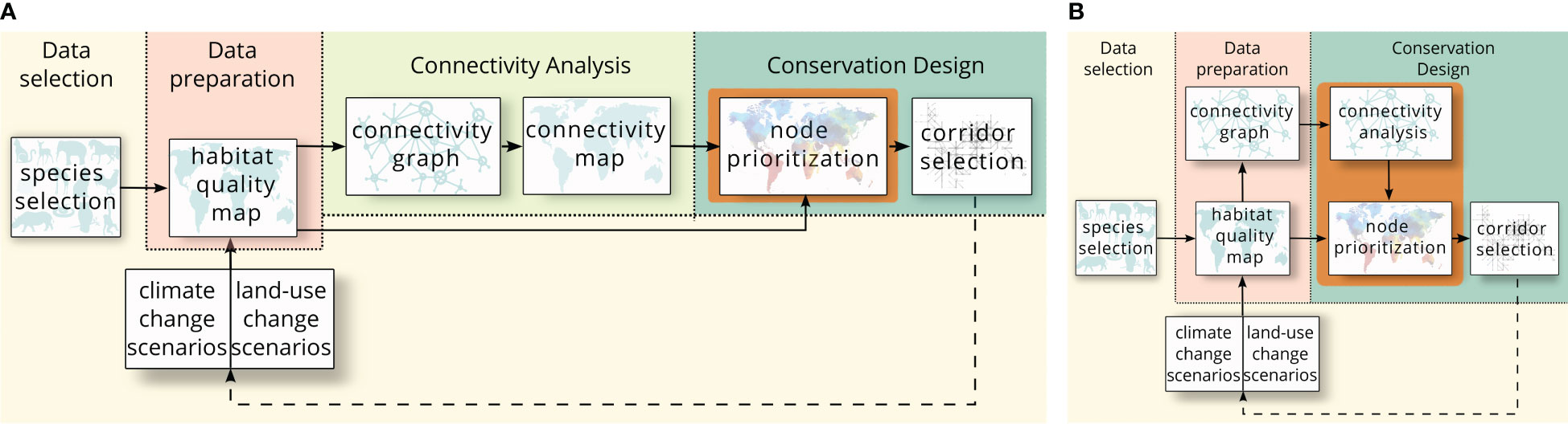
Figure 1 The workflow when connectivity maps need to be created for spatial planning tools (Panel A) such as Marxan and Zonation compared to the workflow of Coco (Panel B). An extra connectivity analysis needs to be performed by the user during the original workflow to generate connectivity maps from the connectivity graphs as input maps for the spatial planning tools. However, since Coco is able to calculate metrics directly from the connectivity graphs, no user-performed analysis is needed.

Here, we present an exact method to directly optimize connectivity metrics during the biodiversity conservation design process. We introduce Coco, an open-source spatial planning DSS to design ecologically connected conservation networks. Figure 1B shows the workflow when using Coco. Instead of requiring connectivity maps, Coco can use connectivity graphs as input and run connectivity metrics on them. Coco then uses the resulting (vertex- or edge-weighted) connectivity values in the optimization. This removes the extra step of having to create connectivity maps. Additionally, because Coco requires a graph instead of a map, connectivity metrics generating edge values can also be used, without the need to be rewritten into a vertex-weighted variant.

In addition to treating the result of the connectivity analysis as a feature map, Coco provides optimal ILP solutions to solve different variations of the RSP that directly optimize the connectivity metrics. Consequently, more emphasis is placed on connectivity during the spatial planning phase of SCP.

First, we describe the existing formulation to include vertex-weighted values as connectivity features in RSP. We differentiate between vertex-weighted connectivity metrics and edge-weighted connectivity metrics and introduce RSP formulations for both.

We continue to introduce two novel variations of RSP that allow direct optimization over connectivity metrics. One variation minimizes cost while maximizing the connectivity metric, and the other maximizes the connectivity metric for a fixed cost. We give all RSP variations as ILPs. We perform benchmark tests on 12 simulated datasets and we test Coco on two real datasets, one smaller dataset and one large-scale data set. We run Coco on the smaller dataset as used by Daigle et al. and show that Coco outperforms Marxan Connect (MC) (Daigle et al., 2020), both in runtime and solution quality, i.e., meeting the required conservation targets at a lower cost. We run Coco on a large-scale dataset of the marine area in British Columbia, Canada, as used in an analysis of the conservation potential (Ban et al., 2013). For our experiments, we use betweenness centrality (BC) (Freeman, 1977) as a vertex-weighted connectivity metric example and equivalent connectivity (EC) (Saura et al., 2011) as an edge-weighted connectivity metric example. We explain the ecological importance of both BC and EC, and give their formal graph-theoretical definitions. We show that in all cases directly optimizing over connectivity metrics results in higher connectivity values at a lower cost, while maintaining the same feature occurrence.

2 Materials and methods

2.1 Reserve selection problem

Coco can solve different variants of RSP, which aims to select specific sites for conservation from a set of potential sites. Various formulations of RSP exist (Williams et al., 2005), e.g., as a Maximal Covering problem (Church et al., 1996; Arthur et al., 1997) or a probabilistic model (Billionnet, 2011).

Here, our basis is a cost-based RSP formulation (Rodrigues et al., 2000), variations of which are widely used (Ball et al., 2009; Beyer et al., 2016; Daigle et al., 2020; Hanson et al., 2022). A grid overlay or existing geographical, administrative or ecological boundaries divides the landscape into smaller discrete spatial units, i.e., pixels. Each pixel has an associated cost, e.g., acquisition cost, percentage of the total landscape, or socio/economic cost. Further, it contains information on the occurrence of each feature, e.g., species, in that pixel. The goal is to minimize the cost while keeping the occurrence of each feature above a specified threshold, i.e., the target. More formally, let N be the set of pixels. For each pixel i ∈ N, we introduce a decision variable x_i indicating whether pixel i is in the solution (x_i = 1) or not (x_i = 0) and a variable c_i indicating the cost associated with pixel i. Further, let K be the set of selected features, then for each pixel i ∈ N and each feature k ∈ K, we define r_ik as the occurrence of feature k in pixel i. Additionally, for each feature k ∈ K we let T_k be the target to reach for feature k. The cost-based RSP is then defined as follows:

$\begin{array}{ll}\begin{array}{cc}\min & {\displaystyle \sum _{i=1}^N{c}_i{x}_i}\end{array}& (1)\end{array}$

$\begin{array}{ll}\begin{array}{cc}\text{s}.\text{t}.{\displaystyle \sum _{i=1}^N{r}_{ik}{x}_i}\ge T_k& \forall k\in K\end{array}& (2)\end{array}$

$\begin{array}{ll}\begin{array}{cc}{x}_i\in \{0,1\}& \forall i\in N\end{array}& (3)\end{array}$

The objective function (1) minimizes the cost of all selected pixels, while constraint (2) enforces the occurrence target for each feature to be met. Constraint (3) indicates that all x_i are binary decision variables, i.e., they can only be 0 or 1. Note that our problem formulation (1)–(3) of RSP is already given as an ILP and bears a strong similarity to a multidimensional knapsack problem. The number of possible selections grows exponentially with an increasing number of pixels, quickly rendering it impossible for a computer to try them all out. It is actually easy to show that RSP is NP-hard because of its similarity to knapsack-like problems. This means that it is highly unlikely that an algorithm exists that always returns an optimal selection of pixels in time polynomial in the input size. See (Garey and Johnson, 1979) for a more detailed explanation of the theory behind NP-hardness and the Supplementary Information 2 section of this article for a formal NP-hardness proof of RSP. Nevertheless, despite its theoretical intractability, even large instances of this knapsack-like problem can be solved to provable optimality by ILP solvers in a short computation time which we also observe in our experimental results.

2.2 Graph-based connectivity metrics

Many connectivity metrics exist to quantify connectivity each with their own strengths and weaknesses (Rayfield et al., 2011; Saura et al., 2018). Simple metrics, like Euclidian distance, while easy to understand and calculate, might be too simplistic to simulate the complex interactions of species movement and landscape structure (Moilanen and Nieminen, 2002). More complex metrics, while ecologically more realistic, might be too computationally expensive (Mancini et al., 2022). Structural connectivity expresses the connectivity between two pixels based on physical features and habitat arrangements of the landscape (Keeley et al., 2021). Structural connectivity metrics can, for example, be based on the presence of corridors or stepping stones (Freeman, 1977), on distances (Klein and Randić, 1993), or on habitat availability in the landscape (Kindlmann and Burel, 2008). Functional connectivity indicates the degree to which a landscape impairs or facilitates the movement of focal species, considering each species’ perception separately (Arkilanian et al., 2020; Keeley et al., 2021). Functional connectivity metrics include metrics based on movement probability between patches, and immigration rates (Kindlmann and Burel, 2008). Many ecological connectivity metrics exist (Pascual-Hortal and Saura, 2006; McRae et al., 2008; Prugh, 2009; Keeley et al., 2018). Selecting suitable connectivity metrics depends on expert opinion, data availability and conservation goals. The conservation goals heavily depend on the amount of existing human modification of the conservation planning area (Belote et al., 2019; Locke et al., 2019). As such, the amount of human modification is a factor to take into account when selecting suitable connectivity metrics (Keeley et al., 2021).

To solve different variations of the RSP on a given planning area, we mathematically represent the area as a graph G = (V, E). A graph G consists of a set V of elements called vertices and a set E of relations between pairs of vertices in V called edges. Each vertex v ∈ V represents exactly one discrete, indivisible spatial unit, i.e., pixel i ∈ N. The size of each pixel depends on the chosen resolution for the pixels of the landscape. The set of edges E represents connectivity links between the pixels. These connectivity links indicate either structural or functional connectivity. Graph-based connectivity metrics can be either vertex-weighted, e.g., BC and in-degree, or edge-weighted, e.g., EC and Euclidian distance. Vertex-weighted metrics assign a weight to each vertex v ∈ V, i.e., each pixel. Edge-weighted metrics assign a weight to each edge e ∈ E, or to each pair of vertices (v_i, v_j) ∈ V in the graph. Ecologically, edge weights can represent functional or structural distances between pixels. Coco currently offers a handful of connectivity metrics, such as BC and EC (Section 3.2). However, Coco can be expanded to include any metric that can be represented as either a vertex-weighted or edge-weighted connectivity metric. Since grids are a special graph type, Coco can include grid-based metrics as well.

2.3 Connectivity data in Coco

Coco is able to run several variations of the RSP to include connectivity in the conservation area selection. Coco is written in Python and calls the ILP solver Gurobi to solve the ILP formulations of the user-selected RSP variation on the data. Coco is open-source and freely available on https://github.com/esvanmantgem/coco under a GPLv3 license. Coco requires input very similar to Marxan (Ball et al., 2009). It needs the pixels of the area, including cost and feature occurrence data for each pixel where the feature is present.

In addition, Coco requires connectivity data. Including connectivity in RSP requires the integration of the results of the connectivity analysis into the RSP formulation. For this, connectivity data provides the information to generate a directed or undirected graph G = (V, E) needed for use in the connectivity metrics. The connectivity data can be a (weighted) connectivity matrix or a (weighted) edge list per feature. Both data formats contain information about the edges connecting vertices and possible weights on the edges. The connectivity data can either represent the complete graph of the planning area or a subgraph, such as the networks created in the habitat network definition phase of the conservation area selection stage. Optionally, in case pixel attributes, i.e., vertex weights, are used in metrics, data containing the attribute values for each pixel, i.e., the weights of the vertices, should be provided. The connectivity data can provide one connectivity matrix or edge list containing the collapsed information for all features k ∈ K, or k datasets, one dataset per feature. As such, Coco can optimize connectivity metrics while taking each feature into account individually. It calculates the user-selected connectivity metrics on the connectivity data before starting the ILP solver to find an optimal solution. Tools like Circuitscape (McRae et al., 2008), Grainscape (Chubaty et al., 2020), and Conefore (Saura and Torné, 2009) offer functionality to create the connectivity data.

2.4 Including Connectivity in RSP

Since not all features are present in every pixel, we define P_k ⊆ P as the set of pixels containing feature k. For each feature k, we generate a graph G_k = (V_k, E_k), such that V_k contains a vertex v_i for each pixel i ∈ P_k and E_k contains an edge e_ij for each link in the connectivity data of feature k. Additionally, let 𝒱 be the set of all vertex-weighted metrics and ℰ the set of all edge-weighted metrics to be considered. Given a graph G_k = (V_k, E_k), vertices v_i, v_j ∈ V and edge (V_i, V_j) ∈ E, we define w_mik to be the value of vertex-weighted metric m ∈ 𝒱 applied to the connectivity data of feature k and vertex v_i. Similarly, we define w_mijk to be the value of edge-weighted metric m ∈ ℰ applied to the connectivity data of feature k and edge e_ij = (v_i, v_j).

2.4.1 RSP with connectivity features

A straightforward way of including the connectivity values, i.e., evaluation of the connectivity metrics, in RSP is to model them using connectivity features (Daigle et al., 2020). We call this strategy RSP with Connectivity Features (RSP-CF). We ensure that each connectivity feature, i.e., each connectivity metric m∈ 𝒱 ∪ ℰ per feature k, reaches a predefined target T_mk. For this, we sum the connectivity values w_mik or w_mijk resulting from the evaluation of each metric m for each feature k for each vertex V_i or edge e_ij, respectively. We add constraint (4) for vertex-weighted connectivity metrics in 𝒱 and constraint (5) for edge-weighted connectivity metrics in ℰ:

$\begin{array}{ll}\begin{array}{cc}{\displaystyle \sum _{{\upsilon }_i\in V_k}{w}_{mik}}{x}_i\ge T_{mk}& \forall m\end{array}\in 𝒱,\forall k\in K& (4)\end{array}$

$\begin{array}{ll}\begin{array}{cc}{\displaystyle \sum _{e_{ij}\in E_k}{w}_{mijk}}{x}_i{x}_j\ge T_{mk}& \forall m\end{array}\in \epsilon ,\forall k\in K& (5)\end{array}$

For vertex-weighted metrics, we only need to include the metric evaluation of vertex v_i if pixel x_i is in the solution. Thus, we multiply w_mik by the decision variable x_i. While constraint (4) for vertex-weighted metrics is an ILP, formalizing constraints (5) for edge-weight metrics as an ILP is slightly more complicated. The connectivity values resulting from the edge-weighted metric evaluation correspond to edges e_ij ∈ E_k with v_i, v_j ∈ V_k. We must ensure we only include edge values if both vertices incident to the edge are in the solution. Thus, we multiply the connectivity value w_mijk by the decision variables x_i, x_j of both vertices v_i, v_j, leading to the non-linear term w_mijkx_ix_j. To linearize this part of the constraint, we introduce a binary variable z_ij that is 1 if and only if both x_i and x_j are 1, i.e., is 1 only if both pixels i and j are in the solution. To enforce this, we add constraints (10)-(12) and replace constraint (5) with constraint (9). The complete ILP formulation to include connectivity as a feature is as follows:

$\begin{array}{ll}\min {\displaystyle \sum _{i=1}^N{c}_i}{x}_i& (6)\end{array}$

$\begin{array}{ll}\begin{array}{cc}\text{s}.\text{t}.\hspace{1em}{\displaystyle \sum _{i=1}^N{r}_{ik}{x}_i}\ge T_k& \forall k\in K\end{array}& (7)\end{array}$

$\begin{array}{ll}\begin{array}{cc}{\displaystyle \sum _{{\upsilon }_i\in V_k}{w}_{mik}{x}_i}\ge T_{mk}& \forall m\end{array}\in 𝒱,\forall k\in K& (8)\end{array}$

$\begin{array}{ll}\begin{array}{cc}{\displaystyle \sum _{e_{ij}\in E_k}{w}_{mijk}{z}_{ij}}\ge T_{mk}& \forall m\in ℰ,\forall k\in K\end{array}& (9)\end{array}$

$\begin{array}{ll}\begin{array}{cc}{z}_{ij}\ge x_i+x_j-1& \forall z\end{array}& (10)\end{array}$

$\begin{array}{ll}\begin{array}{cc}{z}_{ij}\le x_i& \forall z\end{array}& (11)\end{array}$

$\begin{array}{ll}\begin{array}{cc}{z}_{ij}\le x_j& \forall z\end{array}& (12)\end{array}$

$\begin{array}{ll}\begin{array}{cc}{x}_i,z_{ij}\in \{0,1\}& \forall x,z\end{array}& (13)\end{array}$

2.4.2 RSP with cost-connectivity

To improve the connectivity in the resulting conservation area, we formulate a variant of RSP that allows direct optimization over the connectivity metrics while still minimizing cost, RSP Cost-Connectivity (RSP-CC). To optimize directly over the connectivity metrics, we need to adjust the objective function (1). We want to minimize the cost of the selected pixels and maximize connectivity values resulting from the evaluation of each connectivity metric m ∈ 𝒱 ∪ ℰ for each feature k. Further, we introduce parameters α and β to balance the weight of the cost against the profit of the connectivity values.

$\begin{array}{ll}\min \alpha {\displaystyle \sum _{i=1}^N{c}_i{x}_i}+\max \beta ({\displaystyle \sum _{m\in 𝒱}{\displaystyle \sum _{k\in K}{\displaystyle \sum _{{\upsilon }_i\in V_k}{w}_{mik}}}}{x}_i+{\displaystyle \sum _{m\in ℰ}{\displaystyle \sum _{k\in K}{\displaystyle \sum _{e_{ij}\in E_k}{w}_{mijk}}}}{z}_{ij})& (14)\end{array}$

To rewrite this objective formulation as an ILP, we need to maximize or minimize the entire objective function. Maximizing a function over its arguments is mathematically equivalent to minimizing the function over the same arguments with a sign change, i.e., the negative. As such, we can rewrite the connectivity maximization as $\min -\beta ({\displaystyle {\sum }_{v_i\in V_k}{w}_{mik}+{\displaystyle {\sum }_{e_{ij}\in E_k}{w}_{mijk}}})$ for all metrics.

The following ILP formulation for RSP includes connectivity optimization:

$\begin{array}{ll}\min \alpha {\displaystyle \sum _{i=1}^N{c}_i{x}_i-\beta \left({\displaystyle \sum _{m\in 𝒱}{\displaystyle \sum _{k\in K}{\displaystyle \sum _{v_i\in V_k}{w}_{mik}{x}_i+{\displaystyle \sum _{m\in ℰ}{\displaystyle \sum _{k\in K}{\displaystyle \sum _{e_{ij}\in E_k}{w}_{mijk}{z}_{ij}}}}}}}\right)}& (15)\end{array}$

$\begin{array}{ll}\begin{array}{cc}\text{s}.\text{t}.{\displaystyle \sum _{i=1}^N{r}_{ik}{x}_i}\ge T_k& \forall k\in K\end{array}& (16)\end{array}$

$\begin{array}{ll}(10),(11),(12),(13)& (17)\end{array}$

2.4.3 RSP with cost budget and connectivity

In specific circumstances, it might not be necessary to minimize cost, e.g., when expanding an existing conservation area to include an additional selected area that is a specified maximum percentage of the entire planning area or with a fixed cost. In cases like this, setting a maximum cost C is sufficient. For this, we also define an ILP formulation to optimize directly over connectivity metrics without minimizing cost and instead include the cost as a constraint, RSP with Cost Budget and Connectivity (RSP-CBC).

$\begin{array}{ll}\max {\displaystyle \sum _{m\in 𝒱}{\displaystyle \sum _{k\in K}{\displaystyle \sum _{{\upsilon }_i\in V_k}{w}_{mik}}}}{x}_i+{\displaystyle \sum _{m\in ℰ}{\displaystyle \sum _{k\in K}{\displaystyle \sum _{e_{ij}\in E_k}{w}_{mijk}}}}{z}_{ij}& (18)\end{array}$

$\begin{array}{ll}\text{s}.\text{t}.{\displaystyle \sum _{i=1}^N{c}_i{x}_i}\le C& (19)\end{array}$

$\begin{array}{ll}\begin{array}{cc}{\displaystyle \sum _{i=1}^N{r}_{ik}{x}_i}\ge T_k& \forall k\in K\end{array}& (20)\end{array}$

$\begin{array}{ll}(10),(11),(12),(13)& (21)\end{array}$

Here, the objective function (18) maximizes the connectivity values resulting from the evaluation of the connectivity metrics while making sure the cost of the selected pixels, c_ix_i does not exceed the maximum allowed cost C, constraint (19).

3 Results

3.1 Experimental results

We ran several experiments to test the performance of Coco, both regarding runtime and solution quality, i.e., cost and metric values. We ran all experiments on an AMD EPYC 7742 64-Core Processor, 128 threads, and 1TB RAM. We tested the different variations of the RSP on 12 simulated datasets and two real datasets. We ran all different versions of RSP with both BC, EC, and BC+EC and evaluated the solution quality in terms of cost and metric values. We generated the datasets to increase in size, both the planning area size and the number of features, to additionally test the runtime performance of Coco. To compare against MC (Daigle et al., 2020), we ran Coco on their dataset of the Great Barrier Reef (Great Barrier Reef Marine Park Authority, 2001) and compared our findings to the results of MC. Since they report findings using BC, we only ran BC as a metric for these experiments. Further, we created a large-scale dataset based on data from the marine area in British Columbia (British Columbia Marine Conservation Analysis Project Team, 2011). We ran the different variations of the RSP using the vertex-weighted BC and the edge-weighted EC as metrics. In both cases, the experimental results reported in this manuscript illustrate the performance and functionalities of Coco. The results are not suitable to inform policy-making or usable as a guideline for the conservation design of the planning areas.

3.2 Betweenness centrality and equivalent connectivity

Currently, Coco has several different connectivity metrics implemented, such as degree centrality, betweenness centrality (Freeman, 1977) and equivalent connectivity. Due to its modular software architecture design, it is straightforward to expand Coco and add additional connectivity metrics. To illustrate the functionality of Coco, we focus on betweenness centrality (BC) Freeman (1977) and equivalent connectivity (EC) (Saura et al., 2011) in our experimental results. Both BC and EC are widely used metrics in conservation design (Gupta et al., 2019; Daigle et al., 2020). Where BC can indicate how well a pixel functions as a stepping stone for both long-range and short-range movement in the conservation area, EC prioritizes high-quality pixels with a high-probability of connectivity, important for the prioritization of high quality habitat patches. BC quantifies the degree to which pixels promote movement between other non-adjacent pixels and, as such, is very suited as a metric for long-range connectivity (Rayfield et al., 2016). More formally, BC is a measure of centrality in a graph based on shortest paths. The shortest path between two vertices of a connected graph is the path between two vertices such that the sum of the weight of the edges is minimal. A shortest path exists for every pair of vertices in a connected graph. The BC of a vertex indicates how many of the shortest paths in a graph go through the vertex. More formally, given a graph G = (V,E) and a vertex υ, the BC of vertex υ is defined as follows:

$$\text{BC}(\upsilon )={\displaystyle \sum _{s,t\in V}\frac{\sigma (s,t|\upsilon )}{\sigma (s,t)}}$$

Here, σ(s, t) indicates the number of shortest paths from s to t and σ(s, t | v) the number of shortest paths from s to t going through v. BC is a vertex-weighted metric since it calculates values per vertex. Note that the edge weights used to calculate the shortest path can represent structural and functional distance.

EC is an edge-weighted metric based on the equivalent connectivity area (ECA) metric (Saura et al., 2011). The ECA is derived from the probability of connectivity (PC) (Saura and Pascual-Hortal, 2007), a habitat availability index that quantifies functional connectivity over the entire conservation area (Saura et al., 2011). It improves several limitations of the PC and provides better interpretability. Saura et al. define the ECA as follows:

$$\text{ECA}=\sqrt{{\displaystyle \sum _{i=1}^N{\displaystyle \sum _{j=1}^N{a}_i{a}_j{p}_{ij}}}}$$

Since we generalize the attributes a_i, a_j to correspond to other habitat characteristics than area alone, we refer to the ECA as EC (Saura et al., 2011). The EC is an edge-weighted connectivity metric calculated on a graph G = (V,E). Let habitat attribute values a_i and a_j be vertex-weights on vertices v_i, v_j ∈ V representing pixels i and j. Further, let p_ij be an edge-weight on edge e_ij ∈ E connecting vertices v_i and v_j representing the links between the pixels. Because the calculation of the EC results in a value on an edge, depending on the weight of two adjacent vertices and on the weight of the edge connecting them, the EC is an edge-weighted metric. To use the EC in spatial prioritization software such as Zonation which is only able to use input maps containing vertex-weighted connectivity metric values, Albert et al. define dEC as the patch importance based on EC (Albert et al., 2017). Each patch is treated as a single vertex in the graph for the connectivity analysis. However, each pixel in the patch is an individual pixel for spatial prioritization. For each patch i, they calculate $d\text{E}{\text{C}}_i=\frac{\text{EC}-\text{E}{\text{C}}_i}{\text{EC}}$, where EC_i is the EC of the area with patch i removed. However, since Coco is able to optimize edge-weighted connectivity metrics directly, we calculate the contribution to the EC for each individual link between two pixels in the connectivity graph. For this, we define the EC_(eij) as follows:

$\begin{array}{ll}\text{EC}(e_{ij})=a_i{a}_j{p}_{ij}& (22)\end{array}$

Here, a_i and a_j represent the values of a habitat attribute of pixels i and j, such as area size, species occurrence, or habitat quality. Further, p_ij indicates the probability of (functional or structural) connectivity between pixels i and j, quantifying the connectivity of the link between pixels i and j. Thus, the EC increases when the probability of connectivity p_ij increases, prioritizing higher-quality vertices with a higher probability of connectivity.

The reason why we focussed on BC and EC during our experiments is twofold. First, since the characteristics of BC and EC complement each other, they are often used together to explore different scenarios in conservation design (Rayfield et al., 2016; Albert et al., 2017). Second, since BC is a vertex-weighted metric and EC an edge-weighted metric, they are suitable to show the ability of Coco to optimize directly over both vertex-weighted metrics and edge-weighted metrics, in contrast to other spatial prioritization software such as Marxan, Zonation and Prioritizr.

3.3 Simulated data

To extensively test the different RSP formulations implemented in Coco we generated 12 datasets that simulate conservation planning areas. Each dataset consists of a feature map of a specified resolution, a connectivity graph based on the feature map and in some cases a quality map needed for the EC. We generated features maps of resolutions 400x400, 500x500 and 1000x1000. First, we initialized 2D grid layouts of the size of the resolution. Then we generated feature population centers by assigning random pixels in the grid a value based on random uniform distribution. To simulate the habitat clusters, we used a gradient function that assigns decreasing feature counts for pixels around the population centers with varying gradient size. Next we generated connectivity graphs based on the feature maps. We selected a subset of habitat pixels with a specified minimal feature occurence as vertices for the connectivity graph. We then used these vertices to create a complete graph using the Euclidean distance in the 2D grid layout as edge-weights. Lastly, we used a Perlin noise function (Perlin, 1985) to sample habitat quality data for use in the EC.

We generated 8 occurrence datasets of sizes 400x400 and 500x500 with 15 features. To find the limits of Coco we generated a large 1000x1000 dataset with binary presence/absence data for 15, 30, 50, and 70 features. Additionally, we generated quality maps for 6 datasets. We ran RSP-CF, RSP-CC and RSP-CBC with BC on all datasets. For the 6 datasets with quality maps we additionally ran all RSP variants with EC and BC+EC.

During all runs, the feature counts were slightly above the predefined targets. This is to be expected as the total feature count should be higher than the target, but as low as possible to minimize cost. This includes the connectivity feature in the RSP-CF runs. In all cases, the RSP-CC and RSP-CBC gave better quality solutions than the RSP-CF in terms of achieved total connectivity value. Table 1 shows the test results of Coco on the simulated datasets. Overall, we saw an average 202%, 84% and 121% increase in connectivity value for the RSP-CC runs for BC, EC and BC+EC respectively. With an average cost increase of 0.67%, 0.84% and 0.97% the achieved average connectivity value per planning unit increased by 211%, 124%, 44%. In no case did the average connectivity value of the RSP-CC decrease when compared to the RSP-CF. Next, we ran all datasets with RSP-CBC. Again, for all datasets, all feature counts were slightly above the targets, similar to the results found when running RSP-CF. Similar to the results of RSP-CC, all runs with RSP-CBC resulted in higher quality solutions, i.e., higher connectivity values, when compared to RSP-CF. For each dataset and each metric, we used the cost reported by the RSP-CF as the max cost for RSP-CBC to ensure a fair comparison. In all cases the RSP-CBC outperformed the RSP-CF in terms of solution quality. On average we found an 40%, 37% and 127% increase in total connectivity value, leading to an average increase of 103%, 64%, 22% per planning unit. All benchmark datasets and a complete table with all results and running times are available in the git repository and as Supplementary Information 3, respectively.

TABLE 1

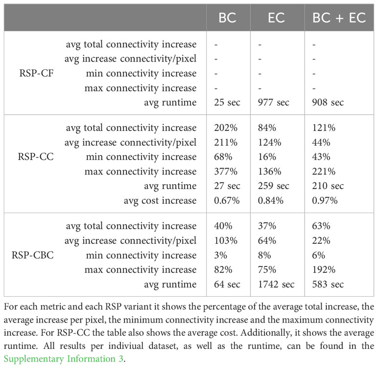
Table 1 Results of tests performed with Coco by running BC, EC and BC+EC on each simulated dataset (12, 6, 6 resp.) for each RSP variant.

3.4 Great Barrier Reef

To evaluate the performance of MC (Daigle et al., 2020), the authors used data of the Great Barrier Reef (Great Barrier Reef Marine Park Authority, 2001). As features, they used 25 bioregions previously identified by Fernandes et al. (Fernandes et al., 2005). As connectivity data, they calculated resistance values for each feature of the planning area. However, instead of using 25 connectivity data sets, i.e., one per feature, they calculated the mean value of each pixel and provided one connectivity edge list for all features. Using this edge list, they calculated the BC for each pixel. They removed all connectivity values below the median value and used the remaining values as a connectivity feature, resulting in 26 features. The planning area used for the experiments by Daigle et al. consists of 321 pixels. The connectivity data resulted in a graph of 321 vertices and 24365 edges. For a direct performance comparison of Coco against MC, we ran Coco RSP-CF with the same data and parameter settings as MC. Since we only use the vertex-weighted BC as a metric, this model is the same as the model of MC. Regarding runtime, Coco spent less than 0.5 sec. to find an optimal solution, while MC needed about 13 sec. to run the heuristic (Table 2).

TABLE 2

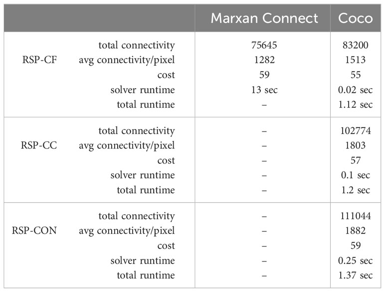
Table 2 Comparison of MC and Coco in term of cost, the total connectivity value (BC) and the average BC per pixel for the selected conservation area. The cost is equal to the size of the conservation area as it was set to 1 for each pixel. Since MC pre-calculates the metric values we measured both the total runtime of Coco and the time spent by the ILP solver in Coco.

To compare the solution quality of the underlying SA heuristic of MC and the exact ILP of Coco we ran all RSP variants on the data. Table 2 shows the experimental results of the solutions for both MC using the RSP-CF variant and for Coco using all three RSP variants. We compared the total cost of the selected conservation area, which is equal to the number of pixels since the cost for each pixel was 1. While both methods reach all predefined feature targets, the smaller solution area of Coco contains 13% more feature occurrences than the larger area found by MC. This extends to the connectivity feature, as Coco reports a total connectivity value of the solution area of 83200, compared to 75645 reported by MC. Since the number of pixels influences the total connectivity value, we additionally calculated the average gained connectivity value per selected pixel, BC/pu, to be able to make a fair comparison. The gain in BC/pu as found by Coco is 18% higher than the the BC/pu of MC. This means, that Coco finds a solution with more protected features, higher connectivity and a lower cost, i.e., in a smaller area.

In addition to a direct comparison of the SA heuristic of MC and the exact ILP method of Coco, we tested the RSP-CC and RSP-CBC on the data. Running RSP-CC on the data increased the cost slightly to 57, while the total connectivity value of the selected area increased significantly, from 83200 to 102774, resulting in a 40% increase in BC/pu. Again, all feature targets were reached.

To gain insight into the optimal connectivity value for the area size found by MC, we also ran RSP-CBC with a fixed cost of 59. Coco found an optimal solution with a 46% increase in the total connectivity value compared to the solution of MC. Additionally, the total feature occurrences protected by the selected area increased with 16.8% when compared to the MC solution.

Figure 2 shows the conservation area of MC (Figure 2A) and the conservation area of Coco RSP-CBC (Figure 2B). Blue pixels are pixels not part of either conservation area. Yellow pixels are those pixels that are selected by both MC and Coco RSP-CBC. These planning areas are mostly large pixels with high feature values, especially the two large pixels in the North, one in the middle and one in the South. The red pixels are those that are selected either by MC (Figure 2A) or Coco RSP-CBC (Figure 2B). A closer examination of these pixels shows that, while the red pixels selected by MC only are more scattered over the entire planning area, those selected by Coco are more strategically placed to create connectivity in the area by means of stepping stones between the pixels with high feature counts. A group of red vertices in the North connects the two large pixels, a big stepping stone cluster of pixels, i.e., a group of selected pixels that are very close to each other, is created in the middle of the area, connecting the South with the North part. Two smaller stepping stone areas are located in the middle of the North and middle clusters and the middle and South clusters.

FIGURE 2

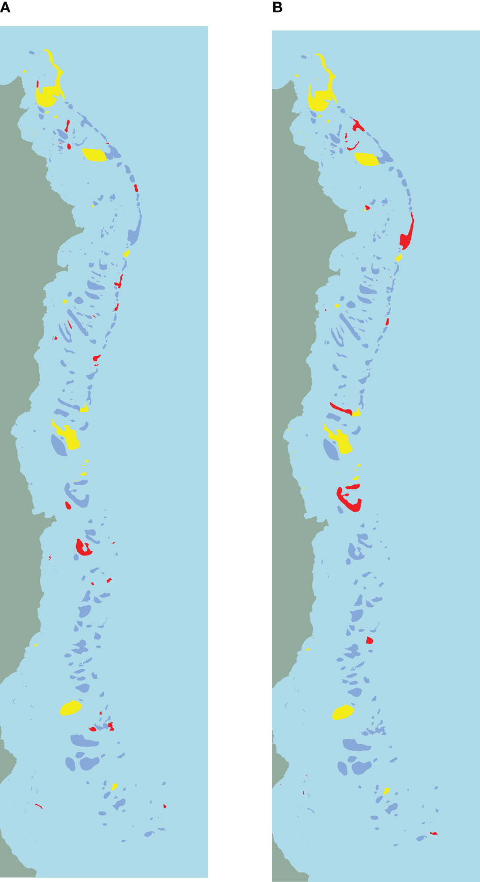
Figure 2 Maps of spatial conservation selections for the Great Barrier Reef. Light-blue (water) and green (land) are not part of the planning area. The dark-blue pixels are not selected for conservation by either MC or Coco, while the yellow areas are selected for conservation by both. The red pixels are selected by either MC (A) or RSP-CBC (B) resp.

These more centalized vertices contribute greatly to overall connectivity of the area as they are at the intersections of many shortest path routes.

3.5 Marine area in British Columbia

To test Coco on a large-scale dataset, we considered a dataset of the marine area in British Columbia used in an analysis of its conservation potential (British Columbia Marine Conservation Analysis Project Team, 2011; Ban et al., 2013). The British Columbia Marine Conservation Analysis team divided the study area into 120,499 square pixels with a side length of two kilometres each and compiled ecological features and data through a series of expert workshops. Here, we consider seven features. We constructed resistance and quality maps for each feature based on human-use data. Next, we created a complete graph containing least-cost paths, i.e., paths with the lowest resistance to movement, between each pair of pixels. The connectivity data yielded 2483 vertices and 2306444 edges over all graphs for each feature. For a more detailed explanation of the data preparation, we refer to the Supplementary Information 1.

We ran all RSP variations using BC, EC, and BC and EC simultaneously (BC+EC). Table 3 shows the important results. Runtimes varied from minutes for the BC runs to less than an hour for the BC+EC runs and, at most 2.5 hours for the EC runs. With a lower cost we found significantly increased connectivity values for all three metric variations for RSP-CC when compared to RSP-CF: with slightly lower cost, the connectivity of the solution area roughly doubled. Running RSP-CBC with the same cost found by the RSP-CF resulted in significantly higher connectivity values. Because of a relatively small cost difference between the RSP-CF and RSP-CC and connectivity values being very close to the optimal value, the differences between the RSP-CC and RSP-CBC runs were only minor. In all tests, the feature targets were exactly reached, apart from the RSP-CBC runs for EC and BC+EC, that had a 1.5% increased feature occurrence when compared to the other found solution areas.

TABLE 3

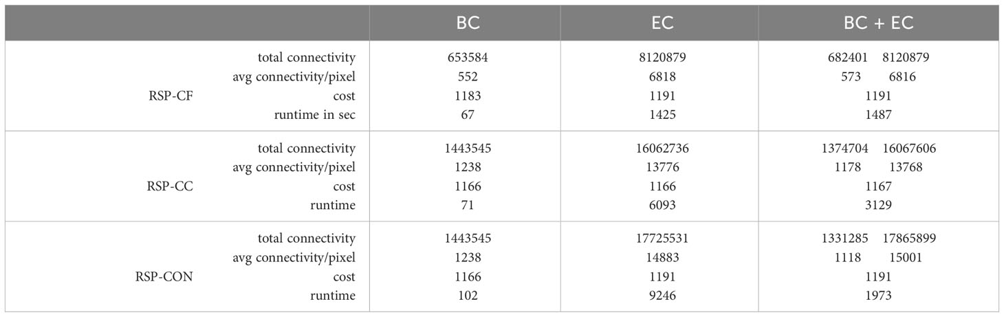
Table 3 Comparison of the different RSP variations in term of cost, the total values and the average metric values per cost for the marine area in British Columbia, Canada.

Where BC is suitable for long-range connectivity, EC should prioritize short-range connectivity. Since we used habitat quality as the attribute of pixels and least-cost paths as a distance relation, a higher total EC should create more clustering of high-quality pixels than a lower total EC. Figure 3 shows the spatial conservation selection maps of BC and EC simultaneously. Here, the selected conservation area should be a mixture of both metrics, creating high-quality habitat clusters with stepping-stone patches between them. The RSP-CF (Figure 3A) shows some features of both metrics, containing some stepping-stone patches from the BC and some habitat clusters from the EC. However, they are still relatively sparse, leaving an abundance of scattered pixels, RSP-CBC (Figure 3B) shows a clear improvement Where the RSP-CF run selected 5 main habitat clusters in the conservation area, the RSP-CBC run removed the large habitat cluster in the West.

FIGURE 3

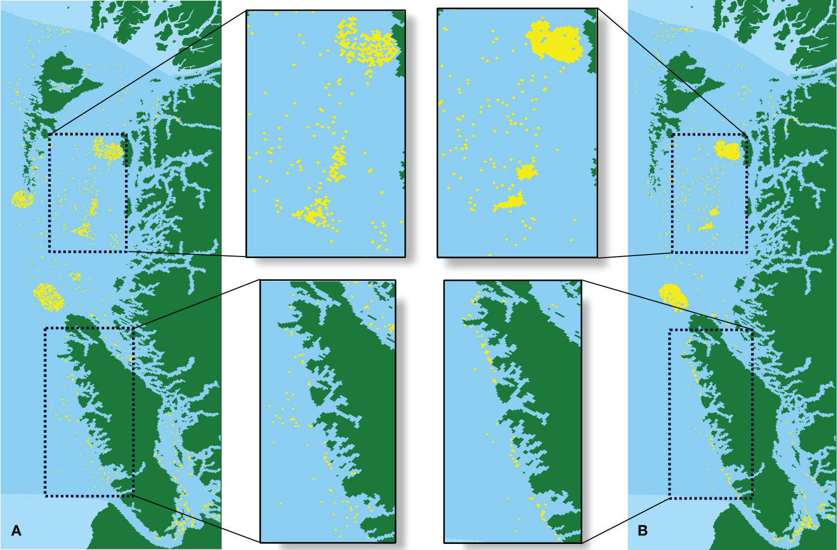
Figure 3 Maps of selected conservation areas for the BCMCA data for (A) RSP-CF with BC+EC and (B) RSP-CBC with BC+EC. Green indicates land and light-blue indicates water, both not part of the planning area. Dark-blue are pixels not selected by Coco for conservation while yellow pixels indicate the selected areas for conservation.

Additionally, part of the planning area. Dark-blue are pixels not selected by Coco for conservation while yellow pixels indicate the selected areas for conservation. the smaller scattered selected areas in the West of the most Northern island are also removed by the RSP-CBC runs. The greater influence of the connectivity metrics in the RSP-CBC run enforced more centrally located areas to be selected, indicating that selecting the extra Western area for conservation would only increase cost, without increasing the connectivity of the entire area or even the feature count. A closer examination of the upper enlarged image shows the influence of EC: instead of the more scattered habitat pixels selected by RSP-CF, RSP-CBC created three dense areas as habitat clusters. The lower enlarged image shows the influence of BC on the solution area: whereas the RSP-CF selected habitat pixels scattered throughout the area, a stepping stone path was selected by RSP-CBC to increase the connectivity between the three big habitat clusters in the middle and the habitat cluster in the South-East of the conservation area.

4 Discussion

4.1 Observations of experimental results

The experimental results described in the previous section clearly show that the exact ILP implementation of RSP-CF in Coco provides higher quality results, i.e., cost and connectivity values, than the heuristic SA implementation of MC. Moreover, the ILPs of RSP-CC and RSPCBC implemented in Coco generate higher connectivity values with lower costs than the ILP implementation of RSP-CF. As such, RSP-CC and RSP-CBC are the superior methods in case connectivity plays a crucial role in the conservation area design. The difference between the RSP-CC and RSP-CBC solutions was minimal, caused by setting the cost of the RSP-CBC to the optimal cost found by RSP-CF, which was close to the minimal cost found by RSP-CC. It shows that RSP-CC offers solutions close to optimal connectivity with minimal cost and provides a strong alternative in case a fixed cost is unknown. Another observation was the difference in runtime between the vertex-weighted BC and the edge-weighted EC. Edge-weighted metrics are harder to solve for the ILP solver due to their inherent non-linear nature making edge-weighted metrics computationally more expensive; this should be a factor when selecting edge-weighted metrics for conservation design.

4.2 Limitations and future work

Coco is a spatial planning tool used for the conservation area selection phase of SCP. Even when it improves on current state-of-the-art spatial planning tools in terms of solution quality, especially considering connectivity, this is only a small part of the entire conservation management life-cycle. As described in Section 1 and shown in Figure 1, conservation selection is a very complicated process involving many strategies, tools and experts. Conservation management is an iterative process of design, implementation and monitoring, with feedback loops to incorporate different climate-change and land-use change projections. As such, many different tools are needed to succesfully execute conservation efforts. Coco is a very useful, albeit small part of the entire conservation management process.

Another difficulty is the evaluation of the selected areas. Even when using multiple scenarios for land-use change and climate change projects, there is no known ground truth as to what the influence of prioritizing one area over another will be in 50, 100 years. This is a very complex task, with many hard to predict interactions. Even with the existence of evaluation tools, such as Conefor (Saura and Torné, 2009), no absolute guarantees can be given. Another complicating factor is the selection of features, i.e., how to best represent an ecosystem or endangered features when selecting a conservation area. Many different strategies exist ranging from selecting one surrogate species (Meurant et al., 2018) to multispecies selection strategies (Wood et al., 2022). Careful consideration and expert knowledge are necessary to select the preferred strategy for the goals of each conservation effort.

A current shortcoming of Coco is the limited selection of implemented metrics. However, the modular architecture allows for straightforward expansion; we plan the addition of relevant metrics to make Coco a strong competitor for other decision-support tools. Another issue is that Coco optimizes the metrics over the input connectivity graph, optimizing the metrics over the solution area would very likely yield better results. However, it is mathematically complex and computationally very expensive and currently part of ongoing research. As we show in Section 3, Coco can run multiple metrics simultaneously at equal importance. We plan on improving Coco by allowing the user to balance the importance of each metric individually and per feature. We also found that setting the cost weight requires knowledge of the data and the metrics used. Further investigation and testing are needed to make this easier and more intuitive to understand.

Due to the complexity of and competing interests involved in conservation design, many DSSs apply a scoring function to planning units, ordering the importance of planning units. Currently, Coco produces binary solutions in the sense that pixels are either selected or not. However, it is possible to use ILP to find multiple optimal solutions, i.e., solutions with the same optimal objective value, if they exist. Alternatively, suboptimal solutions within a specified percentage of the optimal objective value could also be reported. The frequency with which pixels are part of a (sub)optimal solution could then form a basis for a scoring function, creating a prioritization of all pixels in the planning area. Addressing this issue is part of current ongoing research.

5 Conclusions

We introduced Coco, an ILP-based framework to integrate connectivity in conservation design. Where existing tools can consider connectivity values as vertex-weighted connectivity features, i.e., connectivity values on pixels, Coco additionally allows connectivity values on relations between pixels, i.e., edge-weighted values. Moreover, we introduced a novel method to integrate connectivity metrics in conservation design by optimizing directly over vertex-weighted and edge-weighted connectivity metrics, either with cost minimization or a fixed cost. We showed that the conservation areas resulting from optimizing directly over metrics have significantly increased connectivity values, with lower cost when minimizing. The modular architecture of Coco allows for straightforward expansion of the available metrics, making it adaptable to the needs of individual conservation planning efforts.

Data availability statement

The datasets presented in this study can be found in online repositories. The names of the repository/repositories and accession number(s) can be found below: https://github.com/esvanmantgem/coco.

Author contributions

Conceptualization EM and GK; Software EM; Data Preparation – Real Data JH; Data Preparation – Simulated Data LR, EM, JH; Writing – Original Draft EM – Review & Editing EM, JH, GK; Supervision GK.

Funding

The author/s declare financial support was received for the research, authorship, and/or publication of this article. Funded by the Deutsche Forschungsgemeinschaft (DFG, German Research Foundation) under Germany’s Excellence Strategy – EXC-2048/1 – project ID 390686111.

Conflict of interest

The authors declare that the research was conducted in the absence of any commercial or financial relationships that could be construed as a potential conflict of interest.

Publisher’s note

All claims expressed in this article are solely those of the authors and do not necessarily represent those of their affiliated organizations, or those of the publisher, the editors and the reviewers. Any product that may be evaluated in this article, or claim that may be made by its manufacturer, is not guaranteed or endorsed by the publisher.

Supplementary material

The Supplementary Material for this article can be found online at: https://www.frontiersin.org/articles/10.3389/fevo.2023.1149571/full#supplementary-material

Supplementary Information 1 | Description of the Great Barrier Reef dataset.

Supplementary Information 2 | Hardness proof for the Reserve Selection problem.

Supplementary Information 3 | Simulated dataset results.

References

Albert C. H., Rayfield B., Dumitru M., Gonzalez A. (2017). Applying network theory to prioritize multispecies habitat networks that are robust to climate and land-use change. Conserv. Biol. 31, 1383–1396. doi: 10.1111/cobi.12943

PubMed Abstract | CrossRef Full Text | Google Scholar

Arkilanian A., Larocque G., Lucet V., Schrock D., Denépoux C., Gonzalez A. (2020). A review of ecological connectivity analysis in the region of resolution 40-3. Rep. presented to Ministère la faune la forêt Des. parcs du Québec New Engl. Governors Eastern Can. Premiers work. group Ecol. connect 79.

Google Scholar

Arthur J. L., Hachey M., Sahr K., Huso M., Kiester A. (1997). Finding all optimal solutions to the reserve site selection problem: formulation and computational analysis. Environ. Ecol. Stat 4, 153–165. doi: 10.1023/A:1018570311399

CrossRef Full Text | Google Scholar

Ayram C. A. C., Mendoza M. E., Etter A., Salicrup D. R. P. (2016). Habitat connectivity in biodiversity conservation: A review of recent studies and applications. Prog. Phys. Geogr.: Earth Environ. 40, 7–37. doi: 10.1177/0309133315598713

CrossRef Full Text | Google Scholar

Ball I. R., Possingham H. P., Watts M. (2009). Marxan and relatives: software for spatial conservation prioritisation. Spatial Conserv. prioritisation: Quantitative Methods Comput. Tools, 185–195.

Google Scholar

Ban N. C., Bodtker K. M., Nicolson D., Robb C. K., Royle K., Short C. (2013). Setting the stage for marine spatial planning: Ecological and social data collation and analyses in Canada’s pacific waters. Mar. Policy 39, 11–20. doi: 10.1016/j.marpol.2012.10.017

CrossRef Full Text | Google Scholar

Belote R. T., Beier P., Creech T., Wurtzebach Z., Tabor G. (2019). A framework for developing connectivity targets and indicators to guide global conservation efforts. BioScience 70, 122–125. doi: 10.1093/biosci/biz148

PubMed Abstract | CrossRef Full Text | Google Scholar

Bennett G. (2004). Integrating biodiversity conservation and sustainable use: lessons learned from ecological networks (IUCN).

Google Scholar

Bennett G., Mulongoy K. J. (2006). Review of experience with ecological networks, corridors and buffer zones. Secretariat Convention Biol. Divers. Montreal Tech. Series. 23, 100.

Google Scholar

Beyer H. L., Dujardin Y., Watts M. E., Possingham H. P. (2016). Solving conservation planning problems with integer linear programming. Ecol. Model. 328, 14–22. doi: 10.1016/j.ecolmodel.2016.02.005

CrossRef Full Text | Google Scholar

Billionnet A. (2011). Solving the probabilistic reserve selection problem. Ecol. Model. 222, 546–554. doi: 10.1016/j.ecolmodel.2010.10.009

CrossRef Full Text | Google Scholar

British Columbia Marine Conservation Analysis Project Team (2011) Marine atlas of pacific Canada: A product of the british columbia marine conservation analysis. Available at: www.bcmca.ca.

Google Scholar

Chubaty A. M., Galpern P., Doctolero S. C. (2020). The r toolbox grainscape for modelling and visualizing landscape connectivity using spatially explicit networks. Methods Ecol. Evol. 11, 591–595. doi: 10.1111/2041-210X.13350

CrossRef Full Text | Google Scholar

Church R. L., Stoms D. M., Davis F. W. (1996). Reserve selection as a maximal covering location problem. Biol. Conserv. 76, 105–112. doi: 10.1016/0006-3207(95)00102-6

CrossRef Full Text | Google Scholar

Cook C. N., Inayatullah S., Burgman M. A., Sutherland W. J., Wintle B. A. (2014). Strategic foresight: how planning for the unpredictable can improve environmental decision-making. Trends Ecol. Evol. 29, 531–541. doi: 10.1016/j.tree.2014.07.005

PubMed Abstract | CrossRef Full Text | Google Scholar

Crooks K. R., Sanjayan M. (2006). Connectivity conservation: maintaining connections for nature. Conserv. Biol. 1–20. doi: 10.1017/CBO9780511754821.001

CrossRef Full Text | Google Scholar

Cushman S. A., Landguth E. L., Flather C. H. (2013). Evaluating population connectivity for species of conservation concern in the american great plains. Biodivers. Conserv. 22, 2583–2605. doi: 10.1007/s10531-013-0541-1

CrossRef Full Text | Google Scholar

Daigle R. M., Metaxas A., Balbar A. C., McGowan J., Treml E. A., Kuempel C. D., et al. (2020). Operationalizing ecological connectivity in spatial conservation planning with marxan connect. Methods Ecol. Evol. 11, 570–579. doi: 10.1111/2041-210X.13349

CrossRef Full Text | Google Scholar

Fernandes L., Day J., Lewis A., Slegers S., Kerrigan B., Breen D., et al. (2005). Establishing representative no-take areas in the great barrier reef: Large-scale implementation of theory on marine protected areas. Conserv. Biol. 19, 1733–1744. doi: 10.1111/j.1523-1739.2005.00302.x

CrossRef Full Text | Google Scholar

Freeman L. C. (1977). A set of measures of centrality based on betweenness. Sociometry 40, 35–41. doi: 10.2307/3033543

CrossRef Full Text | Google Scholar

Garey M. R., Johnson D. S. (1979). Computers and Intractability: A Guide to the Theory of NP-Completeness. Ed. Freeman W. H.

Google Scholar

Gaston K., Pressey R., Margules C. R. (2002). Persistence and vulnerability: retaining biodiversity in the landscape and in protected areas. J. Biosci. 27, 361–384. doi: 10.1007/BF02704966

PubMed Abstract | CrossRef Full Text | Google Scholar

Gibson F. L., Rogers A. A., Smith A. D., Roberts A., Possingham H., McCarthy M., et al. (2017). Factors influencing the use of decision support tools in the development and design of conservation policy. Environ. Sci. Policy 70, 1–8. doi: 10.1016/j.envsci.2017.01.002

CrossRef Full Text | Google Scholar

Great Barrier Reef Marine Park Authority (2001) Marine bioregions of the great barrier reef (reef) (v2.0). Available at: http://www.gbrmpa.gov.au/geoportal.

Google Scholar

Groves C. R., Game E. T., Anderson M. G., Cross M., Enquist C., Ferdana Z., et al. (2012). Incorporating climate change into systematic conservation planning. Biodivers. Conserv. 21, 1651–1671. doi: 10.1007/s10531-012-0269-3

CrossRef Full Text | Google Scholar

Gupta A., Dilkina B., Morin D. J., Fuller A. K., Royle J. A., Sutherland C., et al. (2019). Reserve design to optimize functional connectivity and animal density. Conserv. Biol. 33, 1023–1034. doi: 10.1111/cobi.13369

PubMed Abstract | CrossRef Full Text | Google Scholar

Haddad N. M., Brudvig L. A., Clobert J., Davies K. F., Gonzalez A., Holt R. D., et al. (2015). Habitat fragmentation and its lasting impact on earth's ecosystems. Sci. Adv. 1, e1500052. doi: 10.1126/sciadv.1500052

PubMed Abstract | CrossRef Full Text | Google Scholar

Hanski I.. (1999). Metapopulation ecology (Oxford University Press).

Google Scholar

Hanson J. O., Schuster R., Morrell N., Strimas-Mackey M., Edwards B. P. M., Watts M. E., et al. (2022) prioritizr: Systematic Conservation Prioritization in R. Available at: https://github.com/prioritizr/prioritizr.

Google Scholar

Heller N. E., Zavaleta E. S. (2009). Biodiversity management in the face of climate change: A review of 22 years of recommendations. Biol. Conserv. 142, 14–32. doi: 10.1016/j.biocon.2008.10.006

CrossRef Full Text | Google Scholar

Hilty J., Worboys G. L., Keeley A., Woodley S., Lausche B., Locke H., et al. (2020). Guidelines for conserving connectivity through ecological networks and corridors. Best Pract. protect. area Guidelines Ser. 30, 122. doi: 10.2305/IUCN.CH.2020.PAG.30.en

CrossRef Full Text | Google Scholar

IPBES (2019). Global assessment report on biodiversity and ecosystem services of the Intergovernmental Science-Policy Platform on Biodiversity and Ecosystem Services. doi: 10.5281/zenodo.6417333

CrossRef Full Text | Google Scholar

Keeley A. T., Beier P., Jenness J. S. (2021). Connectivity metrics for conservation planning and monitoring. Biol. Conserv. 255, 109008. doi: 10.1016/j.biocon.2021.109008

CrossRef Full Text | Google Scholar

Keeley A. T. H., Ackerly D. D., Cameron D. R., Heller N. E., Huber P. R., Schloss C. A., et al. (2018). New concepts, models, and assessments of climate-wise connectivity. Environ. Res. Lett. 13, 073002. doi: 10.1088/1748-9326/aacb85

CrossRef Full Text | Google Scholar

Kindlmann P., Burel F. (2008). Connectivity measures: a review. Landscape Ecol. 23, 879–890. doi: 10.1007/s10980-008-9245-4

CrossRef Full Text | Google Scholar

Klein D. J., Randić M. (1993). Resistance distance. J. Math. Chem. 12, 81–95. doi: 10.1007/BF01164627

CrossRef Full Text | Google Scholar

Littlefield C. E., Krosby M., Michalak J. L., Lawler J. J. (2019). Connectivity for species on the move: supporting climate-driven range shifts. Front. Ecol. Environ. 17, 270–278. doi: 10.1002/fee.2043

CrossRef Full Text | Google Scholar

Locke H., Ellis E. C., Venter O., Schuster R., Ma K., Shen X., et al. (2019). Three global conditions for biodiversity conservation and sustainable use: an implementation framework. Natl. Sci. Rev. 6, 1080–1082. doi: 10.1093/nsr/nwz136

PubMed Abstract | CrossRef Full Text | Google Scholar

Lucy A. (2022). Establishing a Post-2020 Global Biodiversity Framework. Impact. 2022(4):4–5. doi: 10.21820/23987073.2022.4.4

CrossRef Full Text | Google Scholar

Mancini F., Hodgson J. A., Isaac N. J. (2022). Co-designing an indicator of habitat connectivity for england. Front. Ecol. Evol. 654. doi: 10.3389/fevo.2022.892987

CrossRef Full Text | Google Scholar

Margules C. R., Pressey R. L. (2000). Systematic conservation planning. Nature 405, 243–253. doi: 10.1038/35012251

PubMed Abstract | CrossRef Full Text | Google Scholar

McRae B. H., Dickson B. G., Keitt T. H., Shah V. B. (2008). Using circuit theory to model connectivity in ecology, evolution, and conservation. Ecology 89, 2712–2724. doi: 10.1890/07-1861.1

PubMed Abstract | CrossRef Full Text | Google Scholar

Meurant M., Gonzalez A., Doxa A., Albert C. H. (2018). Selecting surrogate species for connectivity conservation. Biol. Conserv. 227, 326–334. doi: 10.1016/j.biocon.2018.09.028

CrossRef Full Text | Google Scholar

Moilanen A., Franco A. M., Early R. I., Fox R., Wintle B., Thomas C. D. (2005). Prioritizing multiple-use landscapes for conservation: methods for large multi-species planning problems. Proc. R. Soc. B: Biol. Sci. 272, 1885–1891. doi: 10.1098/rspb.2005.3164

CrossRef Full Text | Google Scholar

Moilanen A., Lehtinen P., Kohonen I., Jalkanen J., Virtanen E. A., Kujala H. (2022). Novel methods for spatial prioritization with applications in conservation, land use planning and ecological impact avoidance. Methods Ecol. Evol. 13, 1062–1072. doi: 10.1111/2041-210X.13819

CrossRef Full Text | Google Scholar

Moilanen A., Nieminen M. (2002). Simple connectivity measures in spatial ecology. Ecology 83, 1131–1145. doi: 10.1890/0012-9658(2002)083[1131:SCMISE]2.0.CO;2

CrossRef Full Text | Google Scholar

Newmark W. D. (1987). A land-bridge island perspective on mammalian extinctions in western north american parks. Nature 325, 430–432. doi: 10.1038/325430a0

PubMed Abstract | CrossRef Full Text | Google Scholar

Pascual-Hortal L., Saura S. (2006). Comparison and development of new graph-based landscape connectivity indices: towards the priorization of habitat patches and corridors for conservation. Landscape Ecol. 21, 959–967. doi: 10.1007/s10980-006-0013-z

CrossRef Full Text | Google Scholar

Peh K. S.-H., Balmford A., Bradbury R. B., Brown C., Butchart S. H., Hughes F. M., et al. (2013). Tessa: A toolkit for rapid assessment of ecosystem services at sites of biodiversity conservation importance. Ecosys. Serv. 5, 51–57. doi: 10.1016/j.ecoser.2013.06.003

CrossRef Full Text | Google Scholar

Perlin K. (1985). An image synthesizer. ACM Siggraph Comput. Graphics 19, 287–296. doi: 10.1145/325165.325247

CrossRef Full Text | Google Scholar

Prugh L. R. (2009). An evaluation of patch connectivity measures. Ecol. Appl. 19, 1300–1310. doi: 10.1890/08-1524.1

PubMed Abstract | CrossRef Full Text | Google Scholar

Rands M. R. W., Adams W. M., Bennun L., Butchart S. H. M., Clements A., Coomes D., et al. (2010). Biodiversity conservation: Challenges beyond 2010. Science 329, 1298–1303. doi: 10.1126/science.1189138

PubMed Abstract | CrossRef Full Text | Google Scholar

Rayfield B., Fortin M.-J., Fall A. (2011). Connectivity for conservation: a framework to classify network measures. Ecology 92, 847–858. doi: 10.1890/09-2190.1

PubMed Abstract | CrossRef Full Text | Google Scholar

Rayfield B., Pelletier D., Dumitru M., Cardille J. A., Gonzalez A. (2016). Multipurpose habitat networks for short-range and long-range connectivity: a new method combining graph and circuit connectivity. Methods Ecol. Evol. 7, 222–231. doi: 10.1111/2041-210X.12470

CrossRef Full Text | Google Scholar

Redford K. H., Coppolillo P., Sanderson E. W., Da Fonseca G. A. B., Dinerstein E., Groves C., et al. (2003). Mapping the conservation landscape. Conserv. Biol. 17, 116–131. doi: 10.1046/j.1523-1739.2003.01467.x

CrossRef Full Text | Google Scholar

Reynolds K. M., Hessburg P. F., Bourgeron P. S. (2014). Making Transparent Environmental Management Decisions Applications of the Ecosystem Management Decision Support System (Berlin, Heidelberg: Springer). doi: 10.1007/978-3-642-32000-2

CrossRef Full Text | Google Scholar

Rodrigues A. S., Orestes Cerdeira J., Gaston K. J. (2000). Flexibility, efficiency, and accountability: adapting reserve selection algorithms to more complex conservation problems. Ecography 23, 565–574. doi: 10.1111/j.1600-0587.2000.tb00175.x

CrossRef Full Text | Google Scholar

Rose D. C., Despot-Belmonte K., Pollard J. A., Shears O., Robertson R. J. (2021). Making an Impact: How to Design Relevant and Usable Decision Support Systems for Conservation (Cham: Springer International Publishing). doi: 10.1007/978-3-030-81085-6_8

CrossRef Full Text | Google Scholar

Saura S., Bertzky B., Bastin L., Battistella L., Mandrici A., Dubois G. (2018). Protected area connectivity: Shortfalls in global targets and country-level priorities. Biol. Conserv. 219, 53–67. doi: 10.1016/j.biocon.2017.12.020

PubMed Abstract | CrossRef Full Text | Google Scholar

Saura S., Estreguil C., Mouton C., Rodríguez-Freire M. (2011). Network analysis to assess landscape connectivity trends: Application to european forest, (1990–2000). Ecol. Indic. 11, 407–416. doi: 10.1016/j.ecolind.2010.06.011

CrossRef Full Text | Google Scholar

Saura S., Pascual-Hortal L. (2007). A new habitat availability index to integrate connectivity in landscape conservation planning: Comparison with existing indices and application to a case study. Landscape Urban Plann. 83, 91–103. doi: 10.1016/j.landurbplan.2007.03.005

CrossRef Full Text | Google Scholar

Saura S., Torné J. (2009). Conefor sensinode 2.2: a software package for quantifying the importance of habitat patches for landscape connectivity. Environ. Model. softwar. 24, 135–139. doi: 10.1016/j.envsoft.2008.05.005

CrossRef Full Text | Google Scholar

Scheffers B. R., Meester L. D., Bridge T. C. L., Hoffmann A. A., Pandolfi J. M., Corlett R. T., et al. (2016). The broad footprint of climate change from genes to biomes to people. Science 354, aaf7671. doi: 10.1126/science.aaf7671

PubMed Abstract | CrossRef Full Text | Google Scholar

Schuster R., Hanson J. O., Strimas-Mackey M., Bennett J. R. (2020). Exact integer linear programming solvers outperform simulated annealing for solving conservation planning problems. PeerJ 8, e9258. doi: 10.7717/peerj.9258

PubMed Abstract | CrossRef Full Text | Google Scholar

Schwartz M. W., Cook C. N., Pressey R. L., Pullin A. S., Runge M. C., Salafsky N., et al. (2018). Decision support frameworks and tools for conservation. Conserv. Lett. 11, e12385. doi: 10.1111/conl.12385

CrossRef Full Text | Google Scholar

Sutherland W. J. (2008). The conservation handbook: research, management and policy (John Wiley & Sons).

Google Scholar

Sutherland W. J., Taylor N. G., MacFarlane D., Amano T., Christie A. P., Dicks L. V., et al. (2019). Building a tool to overcome barriers in research-implementation spaces: The conservation evidence database. Biol. Conserv. 238, 108199. doi: 10.1016/j.biocon.2019.108199

CrossRef Full Text | Google Scholar

Tucker M. A., Böhning-Gaese K., Fagan W. F., Fryxell J. M., Moorter B. V., Alberts S. C., et al. (2018). Moving in the anthropocene: Global reductions in terrestrial mammalian movements. Science 359, 466–469. doi: 10.1126/science.aam9712

PubMed Abstract | CrossRef Full Text | Google Scholar

Wang Y., Fang Q., Dissanayake S. T., Önal H. (2020). Optimizing conservation planning for multiple cohabiting species. PloS One 15, e0234968. doi: 10.1371/journal.pone.0234968

PubMed Abstract | CrossRef Full Text | Google Scholar

Wang Y., Önal H. (2016). Optimal design of compact and connected nature reserves for multiple species. Conserv. Biol. 30, 413–424. doi: 10.1111/cobi.12629

PubMed Abstract | CrossRef Full Text | Google Scholar

Williams J. C., ReVelle C. S., Levin S. A. (2005). Spatial attributes and reserve design models: a review. Environ. Model. Assess. 10, 163–181. doi: 10.1007/s10666-005-9007-5

CrossRef Full Text | Google Scholar

Wilson K. A., Underwood E. C., Morrison S. A., Klausmeyer K. R., Murdoch W. W., Reyers B., et al. (2007). Conserving biodiversity efficiently: what to do, where, and when. PloS Biol. 5, e223. doi: 10.1371/journal.pbio.0050223

PubMed Abstract | CrossRef Full Text | Google Scholar

Wood S. L. R., Martins K. T., Dumais-Lalonde V., Tanguy O., Maure F., St-Denis A., et al. (2022). Missing interactions: The current state of multispecies connectivity analysis. Front. Ecol. Evol. 10. doi: 10.3389/fevo.2022.830822

CrossRef Full Text | Google Scholar

Xue Y., Wu X., Morin D., Dilkina B., Fuller A., Royle J. A., et al. (2017). “Dynamic optimization of landscape connectivity embedding spatial-capture-recapture information,” in Thirty-First AAAI Conference on Artificial Intelligence 31(1). doi: 10.1609/aaai.v31i1.11175(Palo Alto, California USA: AAAI Press).

CrossRef Full Text | Google Scholar